Predicting combined carbon emissions in urban regions considering micro-level enterprise electricity consumption data and macro-level regional data

In the context of “dual carbon” goals, governments need accurate carbon accounting results as a basis for formulating corresponding emission reduction policies. Therefore, this study proposes a combined carbon emission prediction method for urban regions, considering micro-level enterprise electricity consumption data and macro-level regional data. Considering the different applicability of prediction methods and the requirements for the data volume, a region-level carbon emission prediction method based on the long short-term memory neural network is proposed, which takes into account the micro-level electricity–carbon coupling relationship. Additionally, a region-level carbon emission prediction method based on the Stochastic Impacts by Regression on Population, Affluence, and Technology (STIRPAT) is proposed, considering the macro-level economic–carbon coupling relationship. The generalized induced ordered weighted averaging method is employed to assign differential weights to micro- and macro-prediction values, yielding regional carbon emission predictions. An empirical analysis is conducted using a key city in the eastern region as an example, analyzing the main influencing factors and predicting carbon emissions based on relevant data from 2017 to 2021, and the accuracy of the models is analyzed and validated.

1 Introduction

In response to the global climate change challenge, an increasing number of countries are taking measures to reduce carbon dioxide emissions (Shi et al., 2022). China, as one of the largest emitters of carbon dioxide, has committed to achieving carbon neutrality by 2030 and reaching peak carbon emissions by 2060 (DENG et al., 2022; Jiang et al., 2023). To accomplish this dual-carbon goal, China has implemented a series of measures. Carbon emission prediction serves as a guiding factor for industrial energy consumption and structural adjustments with the aim of achieving these goals.

Carbon emission prediction technology provides technical support to governments in formulating carbon reduction policies, and research related to carbon emissions is constantly evolving. Karlsson et al. (2020) applied a participatory integrated assessment methodology to plan the development of the construction sector and estimated net-zero carbon emissions by 2045. Ofosu et al. (2020) used a novel gray prediction model to forecast carbon dioxide emissions in the cement industry in China. Hosseini et al. (2019) employed multiple linear regressions to predict carbon dioxide emissions in Iran in 2030 under different scenarios. LUO et al. (2023a) demonstrated that traditional prediction methods are less effective than machine learning methods in dealing with nonlinear signals, such as carbon emissions data. Yi et al. (2017) conducted research on carbon emission prediction in the construction industry by applying the fuzzy cuckoo search algorithm to optimize support vector machine models. Zhang et al. (2022) proposed a comprehensive material–energy–carbon center, using the concept of a “hub” for carbon flow tracking and carbon accounting in the steel industry production processes. Liu et al. (2022) reviewed the existing annual carbon accounting methods, focused on new developed real-time carbon emission technologies and their current application trends, and presented a framework for the latest near-real-time carbon emission accounting technologies that can be widely used. The aforementioned methods focus on macro-level analysis at the city and provincial levels, while there is limited research on micro-level carbon emission prediction for prefecture-level cities and districts.

Research on the factors influencing carbon emissions is of great significance for the current carbon statistics and policy guidelines. Therefore, it is essential to identify the main influencing factors among numerous factors, extract reliable data indicators, and eliminate redundant information as a reasonable basis for predicting carbon emissions in prefecture-level cities and districts. Wang and Zhao (2018) analyzed the factors influencing residential carbon emissions in different regions of China using an improved Stochastic Impacts by Regression on Population, Affluence, and Technology (STIRPAT) algorithm. Li and Wang (2019) employed the logarithmic mean Divisia index (LMDI) decomposition model to analyze the factors affecting urban carbon emissions and found that the economic scale is the main driver of carbon emission growth in China. Cheng et al. (2023) conducted a macro-level analysis of industrial carbon emissions in China by introducing the time-varying parameters of the LMDI decomposition method with five factors. Li et al. (2023) used the DEMATEL-ISM method to identify 23 influencing factors of carbon emissions in prefabricated buildings and calculate the significance and relationships among these factors.

Carbon emissions from electricity production account for more than 40% of the total carbon emissions in our country’s society, making it one of the main targets for carbon reduction efforts (Li et al., 2022). However, traditional methods for calculating carbon emissions, such as the emission factor and material balance methods, have been found to be inaccurate and unsuitable for an accurate estimation of carbon emissions. These methods fail to provide meaningful data support and guidance.

In summary, we propose a city–regional composite carbon emission prediction method that considers micro-level enterprise electricity data and macro-level district data. Considering the wide coverage and the real-time nature of micro-level enterprise electricity consumption data, we utilize these data to identify key carbon-emitting enterprises. These enterprises are then classified based on their respective industries, and the industrial and regional carbon emissions are calculated accordingly. The dynamic time warping (DTW) technique is employed to assess the association strength among different industries, residential areas, transportation, and regional electricity carbon emissions. We establish a micro-level regional carbon emission prediction model based on long short-term memory (LSTM) networks, which yields micro-level predictions of regional carbon emissions. Considering the accuracy of macro-economic data, we construct a regional carbon emission prediction model based on the human Impact Population, Affluence, and Technology (IPAT) equation and the STIRPAT approach. The STIRPAT model provides the estimates of regional carbon emissions. To combine the predictions from the macro- and micro-levels, we introduce the generalized induced ordered weighted averaging (GIOWA) combination forecasting method. By fitting and learning the accuracy of predictions at different timescales for both macro- and micro-levels, we achieve the precise predictions of regional carbon emissions. In this study, we focus on a key city in the eastern province as the empirical object, analyzing and validating the accuracy and applicability of the proposed city–regional carbon emission prediction and influencing factor analysis methods.

2 Framework for predicting combined carbon emissions in urban areas considering micro-level enterprise electricity data and macro-level regional data

In this research, the regional administrative divisions within a city form the defined boundary for carbon emissions accounting. By recognizing the limited availability of data for forecasting carbon emissions at the sub-city level and the scarcity of analyses on the influencing factors and theoretical foundations for regional-level carbon emission predictions, we propose a framework for predicting composite carbon emissions in urban regions by considering the integration of micro-level enterprise electricity data with macro-level district data. The specific framework, as illustrated in Figure 1, consists of three modules.

FIGURE 1

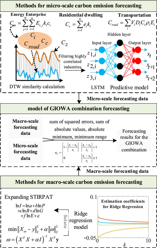
FIGURE 1. Regional carbon emissions forecasting framework.

Module 1: Screening and organizing regional micro-level energy data to establish carbon emission calculation models for various industries, residential areas, and transportation. Utilizing DTW, we calculate the associations among carbon emissions from different industries, residential areas, transportation, and regional electricity carbon emissions. Key electricity-consuming industries are identified using box plots. The LSTM model is employed to train a mapping network that reflects the relationship among strongly correlated industries, residential areas, transportation, and the total regional carbon emissions, enabling the prediction of carbon emissions at the regional level.

Module 2: Constructing a macro-level regional carbon emission prediction model based on the IPAT equation and the STIRPAT approach. Variables such as the population density, per capita regional GDP, energy consumption structure with strong correlations, and the energy intensity in strongly correlated industries are selected as extended variables for the STIRPAT model. The coefficient values for each variable are computed using ridge regression analysis.

Module 3: Establishing a GIOWA combination model. Initial weights are set based on the errors among micro-level predictions, macro-level predictions, and actual data. The results from the micro-level and macro-level predictions are combined using weighted averaging.

3 Calculation of urban regional carbon emissions

The data for carbon emissions in various provinces and cities in China are based on publications, such as the China Urban Statistical Yearbook and the China Energy Statistical Yearbook, released by the National Bureau of Statistics. These statistics include energy consumption and carbon emission data for various industries, cities, and sectors. However, they may not provide detailed information on the energy usage and carbon emissions for specific regions within each city or for key enterprises. This poses significant challenges for Chinese city governments in developing energy saving and emission reduction plans and optimizing industrial structures.

The main causes of urban carbon dioxide emissions are energy consumption and the combustion of fossil fuels. Industrial enterprises are the major consumers in most urban sectors, followed by residential areas (Nie and Kemp, 2014). By obtaining information on the electricity usage from power grid companies and energy consumption data from government departments, we can establish an association model for “electricity consumption–energy consumption–carbon emissions” in energy-consuming enterprises. We can also build a predictive model for carbon emissions in specific regions based on electricity consumption by key enterprises. This model can provide forecasts for urban regional carbon emissions.

3.1 Calculation of urban area carbon emissions

3.1.1 Calculation of carbon emissions from energy-consuming enterprises in urban areas

Industrial fossil fuel consumption is the primary contributor to urban area carbon emissions. The carbon dioxide generated from energy consumption is quantified for energy-intensive enterprises within urban areas using the measurement method outlined in the Guidelines for National Greenhouse Gas Inventories by the Intergovernmental Panel on Climate Change (IPCC). The main formula for calculations within urban regions is given as follows:

$C_m={\displaystyle {\sum }_{j=1}^N}{\displaystyle {\sum }_{i=1}^n}{E}_{i,j}{k}_i{c}_i.(1)$

In the equation, E_i,j represents the energy consumption of the jth enterprise in the ith type of energy in a specific industry. The coefficient k_i corresponds to the conversion factor of the ith energy type into standard coal. The parameter c_i represents the carbon emission coefficient of the ith energy type. Considering the difficulty in obtaining actual energy data for enterprises, we selected electricity, natural gas, and crude oil as the main energy sources for estimation purposes. Referring to the national standard GB/T 4754-2017, Classification of National Economic Industries, energy-consuming enterprises can be categorized into industries such as manufacturing, construction, wholesale, and retail industries.

3.1.2 Calculation of carbon emissions from residential users in the region

In recent years, heat dissipation from residential buildings has decreased. Electricity has become the primary energy source, accounting for approximately 20%–30% of energy consumption in this sector, and along with natural gas, it has witnessed a significant increase (Luo et al., 2023b). The proportion of traditional fossil fuel consumption in residential energy consumption has gradually decreased, while the consumption of liquefied petroleum gas remains relatively stable. Therefore, the calculation formula for the main energy consumption in residential buildings can be divided into electricity, liquefied petroleum gas, and natural gas, and it is given as follows:

$C_c={\displaystyle {\sum }_{i=1}^N}{e}_i{k}_i.(2)$

In the equation, C_c represents the carbon dioxide emissions resulting from residential energy consumption. The variable e_i denotes the usage of different energy types, where e₁ corresponds to electricity usage, e₂ represents natural gas usage, and e₃ stands for liquefied petroleum gas usage. The coefficient k_i corresponds to the carbon emission factors for each energy type.

3.1.3 Calculation of carbon emissions from regional transportation

The carbon emissions calculation for urban regional transportation energy consumption can be approached using a “bottom-up” method. The specific calculation formula is as follows:

$C_{road}={\displaystyle {\sum }_i}{V}_i{D}_i{C}_i{\rho }_i{E}_i,(3)$

where C_road represents the carbon dioxide emission of road traffic in the urban area, kg; V_i is the number of vehicles using fuel i; D_i is the average driving distance of vehicles using fuel i, km; C_i is the fuel consumption of vehicles using fuel i, kg; ρ_i is the default heating value of fuel i; and E_i is the carbon dioxide emission factor of fuel i.

Taking into consideration the intricate and interconnected nature of urban rail transit networks across different cities, it is currently challenging to define the carbon accounting boundaries precisely for rail transit. However, the carbon emissions from rail transit constitute a relatively small proportion of the overall urban carbon emissions. Therefore, allocating the carbon emissions from rail transit to individual regions can be considered negligible compared to emissions from industrial and residential sectors. Consequently, the carbon dioxide emissions from road transportation in urban regions can be utilized as a representation of the transportation-related carbon emissions within a given region.

3.2 Method for predicting regional carbon emissions considering micro-level electricity data

The micro-prediction method is based on micro-data and plays a leading role in prediction. Micro-data are measured on a monthly basis, which is timelier in reflecting the changes in industrial energy consumption and predicting industrial carbon emission trends compared to macro-data, which is measured on an annual basis. On the other hand, the calculation method of micro-carbon emissions can reflect the changes in key carbon-emitting industries within the industry, facilitate the government to formulate reasonable carbon reduction policies, and urge key carbon-emitting enterprises in various industries to rectify their emission levels.

3.2.1 Association degree analysis based on DTW

Different industrial structures and energy structures will lead to different main carbon emission sources in the region. The analysis of the main energy consumption and industrial structure in the region can estimate the carbon emission of the region more quickly, while the carbon emission of each industry is mainly affected by the carbon emission due to the power consumption of the industry (Li and Wang, 2019). Therefore, the correlation between the industry and the total regional carbon emissions can be characterized by calculating the correlation between the industry and the region.

The carbon emissions from the energy usage of industry, residential and transportation, and regional electricity generation are expressed as follows: C_i = {T_i (1), …, T_i(t), …, T_i(n)}, C_c = {T_c (1), …, T_c(t), …, T_c(n)}, C_road = {T_road (1), …, T_road(t), …, T_road(n)}, C_z = {T_z (1), …, T_z(t), …, T_z(n)}; by calculating the Euclidean distance of two sets of data, the distance matrix, D_si, is formed. Taking the distance matrix between the manufacturing industry and the regional carbon emissions as an example, the respective element of the matrix D_si is calculated as follows:

$d\left(n,m\right)=\sqrt{{\left(C_i\left(n\right)-C_z\left(m\right)\right)}^2},(4)$

where C_i(n) and C_z(m) are the nth data in the ith industry carbon cluster and the mth data in the regional carbon cluster, respectively.

An optimal bending path is searched in the matrix D_si so that the sum of the elements on the path is the minimum (Peng et al., 2023). We complete the quantification of similar characteristics, as shown in Eq. 5:

$D_{DTW}\left(T_t,T_{it}\right)=\min \left({\displaystyle {\sum }_{r=1}^L}d\left({\omega }_r\right)\right),(5)$

where ω_r (n,m) represents the coordinate of the rth element in the bending path; L is the number of elements in the bending path, requiring $\max \left(m,n\right)\le L\le mn-1$; d(ω_r) is ω_r, corresponding to d(n,m). From Eq. 5, the similarity of power carbon emissions between various industries and regions is calculated, and the DTW similarity dataset of power carbon emissions from various industries and regional power carbon emissions is established.

To screen for key regional electric power consumption industries, we put forward the quartile box chart method. This uses industry power carbon emissions and regional electric power carbon emissions with a DTW set of four quartiles and the four-quartile value correlation strength threshold (LIU et al., 2021). The generalization ability of sample correlation identification can be improved by taking the quartile and the four-quartile value correlation strength threshold and dividing them by timing data fluctuations and dynamic change. The specific formula is as follows:

$L_{dtw}=L_d+3L_q=L_u+3\left(L_u-L_d\right),(6)$

where L_dtw is the threshold; L_u and L_d are the upper and lower quartiles in the DTW value, respectively; and L_q is the difference between the lower quartile and the upper quartile.

The industries with the greatest influence on regional carbon emissions were selected through the upper- and lower-quartile box chart method. The historical energy consumption data for the industry were used as the training set for the regional carbon emission prediction model.

3.2.2 Prediction method based on the LSTM

An LSTM network used as a carbon emission prediction method is good at processing long sequence data. The energy use data on key industries and historical regional carbon emission data are selected as samples, and the mapping model from “industry energy use data” to “regional carbon emissions” can be obtained through training.

The LSTM network structure consists of the input layer, hidden layer, and output layer. As shown in Figure 2, we send the input information on C_t−1, h_t−1, and x_t to the forgetting gate and memory gate processing, select the forgotten information in C_t-1, and screen the information to be retained in h_t−1 and x_t.

FIGURE 2

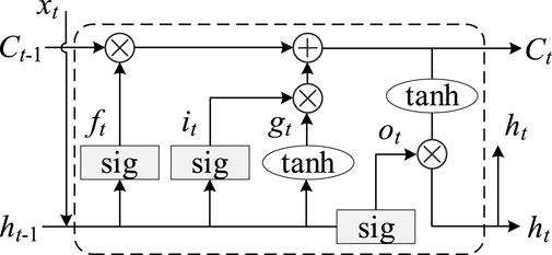
FIGURE 2. Schematic diagram of the long short-term memory (LSTM) structure.

A schematic representation of the internal structure of the LSTM is given in Figure 2. It should be noted that the LSTM structure shown in Figure 2 is only used for a schematic illustration, and the specific level and network number should be adjusted according to the fitting situation.

Assuming that the forgetting gate of each LSTM unit is f_t in time t, the memory gate is i_t and g_t, the output gate is o_t, and the hidden layer state amount is h_t, the update of each gate in time t is given as follows:

$\left\{\begin{array}{c}{f}_t=\left(\sigma (W_f\cdot \left(h_{t-1},x_t\right)+b_f\right)\\ i_t=\left(\sigma (W_i\cdot \left(h_{t-1},x_t\right)+b_i\right)\\ g_t=\tanh \left(\left(Wg\right.\cdot \left(h_{t-1},x_t\right)+b_g\right)\\ o_t=\left(\sigma (W_o\cdot \left(h_{t-1},x_t\right)+b_o\right),\end{array}\right.(7)$

where W_f, W_i, W_g, and W_o are the weight matrices of the input sequence h_t−1 and x_t under each gate, respectively. After processing by the forgetting gate and memory gate, the output signal is generated by the processing of information on the output gates C_t, h_t−1, and x_t:

$h_t=o_t\cdot \tanh \left(f_t\cdot c_{t-1}+i_t\cdot g_t\right).(8)$

3.3 Carbon emission prediction methods considering macro-regional data

Macro-prediction methods are based on macro-data and have a stronger robustness in prediction. Macro-data, measured on an annual basis, can reflect the changes in energy consumption across various industries over the years and have a lower probability of missing data, making it more reliable than micro-data and their predictions. On the other hand, macro-carbon emission prediction can reflect the total carbon emissions of various industries, and compared to micro-carbon emission prediction methods, it can, to some extent, reflect the carbon emission impact of non-key industries.

3.3.1 Predictive model based on the extended STIRPAT

The STIRPAT model introduces multiple-index independent variables on the basis of the IPAT equation to analyze the influence of regional economic indicators, human factors, and the industrial structure on the development of regional carbon emissions.

The STIRPAT model is proposed because of IPAT equality, which is stochastic and scalable. The STIRPAT model, constructed based on the IPAT equality, is expressed as follows:

$I=a\times P^b\times B^c\times T^d\times e,(9)$

where I is the environmental load; P is the population size; B is the economic level; T is the technical level; and b, c, and d are the index items of P, B, and T, respectively. In order to study the factors influencing carbon emissions in urban areas and realize the implementation of energy conservation and emission reduction in urban areas in the future, we extend the STIRPAT model. In these extensions, regional carbon emissions represent the environmental load I, the population density represents the population size P, and the per capita regional GDP represents the economic level B. For the technical level T, we decompose it into the strong correlation industry energy consumption structure G (strong correlation industry energy consumption accounts for the proportion of regional energy consumption) and the strong regional correlation industry energy intensity E (strong correlation industry energy consumption and regional GDP ratio). The extended STIRPAT model can then be represented as follows:

$\ln I=\ln a+b\ln P+c\ln B+d\ln G+f\ln E+\epsilon ,(10)$

where lna is a constant term; ε is a random error term; and b, c, d, and f are the estimated coefficients of population density, per capita regional GDP, strongly related energy consumption structure, and energy intensity of strongly related industries, respectively. To solve the problem of multicollinearity in the regression process of each variable, the ridge regression algorithm was used to solve the problem (Cao et al., 2022).

3.3.2 Ridge regression algorithm

Ridge regression adds a regular term to the loss function of the multivariate linear regression, expressed as the L2 paradigm of the coefficient ω (i.e., the square term of the coefficient) multiplied by the regularization coefficient α. The full expression for the loss function of ridge regression is as follows:

${\min ‖X_{\omega }-y‖}_2^2+\alpha {‖\omega ‖}_2^2.(11)$

The solution is obtained by finding the derivative of the loss function, obtaining the following expression:

$\omega ={\left(X^{T}X+\alpha I\right)}^{-1}{X}^T\mathrm{y}.(12)$

3.4 The GIOWA combination prediction model

Because the combined prediction method of fixed weights cannot reflect the advantage at every time point in the prediction timescale, the ability to learn a model is only limited to the model itself; so, we introduce the GIOWA combination prediction method (Cao et al., 2022). According to the fitting accuracy learning error characteristics of the results of each individual term prediction method, we obtain deeper and more detailed learning from the model. The prediction results of each single-term prediction method at each moment are optimized with the optimization criteria of the minimum sum of errors, the minimum sum of the absolute value of error, and the minimum error minimum, which allow us to obtain combined predicted carbon emissions closer to the real carbon emissions.

For carbon emission prediction, m single-term prediction methods are used. It should be noted that x_t is the measured carbon emission at time t; x_it is the predicted carbon emission at time t in the timescale; g_it is the λ power error at time t in the timescale; g_t = x_t^λ− x_it^λ; and λ = l in this paper. Let W = (w₁, w₂, …, w_m) and T be the weight of the m single-term prediction method in the combined prediction method:

$\begin{array}{c}{a}_{it}=\left\{\begin{array}{cc}1-\left|\frac{x_t-x_{it}}{x_t}\right|& \left|\frac{x_t-x_{it}}{x_t}\right|<1\\ 0& \left|\frac{x_t-x_{it}}{x_t}\right|\ge 1.\end{array}\right.\\ i=1,2,\cdots ,m,t=1,2,\cdots N.\end{array}(13)$

Here, ɑ_it is the prediction accuracy of time point t within the timescale of the i-monomial prediction method. If ɑ_it ∈ [0,1], then ɑ_it is the induced value of predicted carbon emission x_it. An m-monomial prediction method constitutes m two-dimensional arrays ((ɑ_1t, ɑ_1t), (ɑ_2t, ɑ_2t), …, (ɑ_mt, ɑ_mt)), and ɑ_1t, ɑ_2t, …, ɑ_mt are the combined prediction models obtained by the optimization criteria of different error types.

At λ = 1, the GIOWA combined prediction model is the induced ordered weighted arithmetic mean (IOWA) combined prediction model.

${\widehat{x}}_t={\displaystyle {\sum }_{i=1}^m}{w}_i{x}_{it},t=1,2,\cdots ,N.(14)$

The a-index (it) of the conventional weighted arithmetic average at time t is the subscript of the prediction accuracy, expressed as follows:

$f_w\left(〈a_{1t},x_{1t}〉,〈a_{2t},x_{2t}〉,\cdots ,〈a_{mt},x_{mt}〉\right)={\displaystyle {\sum }_{i=1}^m}{w}_i{x}_{\alpha -index\left(it\right)}.(15)$

Then, Eq. 15 is the predicted carbon emission based on the combination of IOWA operators generated at time t by a_1t, a_2t, …, a_mt. By combining the microscopic and macroscopic prediction results and using the GIOWA combination calculation method, the combined prediction results can minimize the sum of error squares, realize the fit with the actual value, and then realize the prediction.

Combination prediction not only inherits the timeliness characteristics of micro-prediction but also inherits the strong robustness of macro-prediction. The learning of the error characteristics based on the fitting accuracy of various single-item prediction methods at different time points in the timescale has a deeper and more detailed understanding of the model. The optimization criteria for the prediction results of each single-item prediction method at each time point are present to minimize the sum of squared errors, absolute sum of errors, absolute value of errors, and extreme difference of errors, to obtain a combination prediction of carbon emissions that is closer to the actual carbon emissions. Compared to traditional carbon emission prediction methods, heterogeneous data sources are more extensive and reflect the energy consumption situation of industries more comprehensively, which inevitably makes the results of combined prediction models more accurate.

4 Results

4.1 Microscopic regional carbon emission prediction based on the LSTM algorithm

This paper takes the state-level new district of an eastern city as the empirical object (hereinafter referred to as region J) to obtain the energy consumption data on the energy-using enterprises in the region from 2020 to 2021, and the region J energy data are obtained from the enterprise survey. Through the proposed carbon emission calculation model, the carbon emissions of energy enterprises in region J are calculated, and the total carbon emission of the region is characterized.

Seven energy sources in region J were selected to calculate their carbon emissions: raw coal, natural gas, gasoline, diesel, liquefied petroleum gas, petroleum coke, and electricity. The total carbon emission from 2017 to 2021 and the carbon emissions of energy-using enterprises are shown in Figure 3. Through Eqs 1-3 and using these seven energy sources and carbon emissions data as training samples for the LSTM, the parameters in the equations are calculated to realize the LSTM in the next prediction.

FIGURE 3

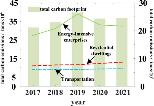
FIGURE 3. Area J. calculation results of enterprises, housing, transportation, and the total carbon emissions.

As shown in Figure 3, the carbon emissions of region J from 2017 to 2021 have increased slowly at first, from 2019 to the maximum point, and then decreased sharply in 2020. As region J is one of the largest modern industrial clusters, with developed manufacturing, steel and petrochemical industries, and large energy consumption, the carbon emissions of energy enterprises account for approximately 58% of their total carbon emissions. The carbon emissions of housing and transportation account for approximately 20% and 17% of the total carbon emissions in the region, respectively. With the outbreak of COVID-19 in 2020, the production capacity of region J energy enterprises decreased, and the energy consumption decreased, resulting in a temporary decline in region J carbon emissions.

The total carbon dioxide emissions of the construction industry are equal to the sum of all the fuel combustion carbon emissions within the industry boundary and the corresponding emissions generated by the electricity and heat purchased by the enterprise, excluding the corresponding emissions used for transport vehicles. The total carbon dioxide emission of the cement production enterprise is equal to the sum of all fuel combustion emissions, process emissions, electricity and heat purchased by the enterprise, and the corresponding emissions of the electricity and heat output of the enterprise. The carbon emission of the transportation industry is mainly divided into two parts: road transportation and urban transportation. Residential carbon emissions are composed of the daily carbon emissions of residents using natural gas in their daily lives and the houses themselves. It should be noted that, except for the transportation industry, the carbon emissions of automobiles used for transportation purposes in other industries belong to the carbon emissions of the transportation industry, rather than being included from the carbon emissions of the industry.

The proportion of the carbon emissions of region J energy-using enterprises in the total carbon emissions of the region is significant. In order to analyze the impact of region J industries on the regional carbon emissions, the energy-using enterprises are divided into different industries, according to the national standard GB/T 4754-2021, Industry Classification of National Economy, and the carbon emissions of various industries are counted, as shown in Table 1.

TABLE 1

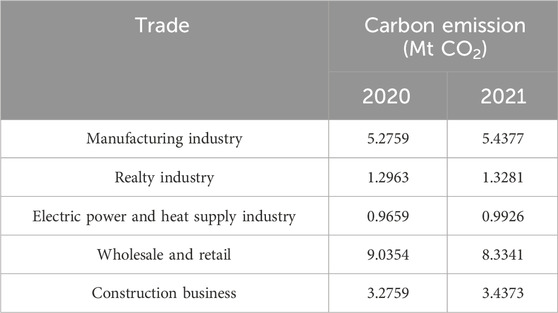
TABLE 1. Total carbon emission of enterprises in various industries in the region J, 2020–2021.

Table 1 lists the key enterprises in the industries with high-electricity carbon emissions from 2020 to 2021. Among them, manufacturing and wholesale and retail occupied 14% and 22% of the carbon emissions of energy enterprises, respectively, while power, heat supply, real estate, and other industries accounted for a relatively low proportion.

The results of screening strongly correlated industries using DTW correlation analysis and employing the upper quartile box plot method are shown in Table 2. According to Table 2, the correlation of region J carbon emissions for industries and regions, manufacturing, wholesale and retail, construction, housing, and transportation are the strong correlation indicators of region J carbon emissions. Therefore, the carbon emission data on each indicator and region in the first 21 months of 2020–2021 in region J were selected as the training set, and the data on the last 3 months from 2020 to 2021 were selected as the test set and by Eqs 7, 8 modeling under LSTM as a prediction algorithm.

TABLE 2

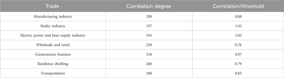
TABLE 2. Correlation between region J and various industries.

To demonstrate the feasibility of using the LSTM algorithm at the micro-level, we introduce the comparative experiment of the particle swarm algorithm, using the average error value to evaluate the superiority of the LSTM algorithm at the micro-level.

Through Table 3, we found that the fitting effect of the LSTM algorithm is better than that of the particle swarm algorithm. In order to ensure the superiority of the algorithm, we set the iterations of the same as 200 iterations.

TABLE 3

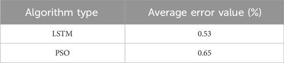
TABLE 3. Comparison of the prediction methods between the LSTM and PSO.

Through the LSTM model, the mapping network of the data on strongly related industries, residential, and traffic carbon emissions to the region was obtained, and the carbon emissions of region J in 2022 was predicted. The predicted results are shown in Figure 4.

FIGURE 4

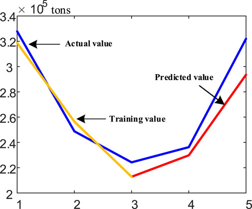
FIGURE 4. Prediction results of carbon emissions in region J, August and December 2021.

Compared with the true carbon emission value obtained through the carbon emission calculation method given in the IPCC guideline, the average error of the trained prediction model in this paper is 0.53% and the prediction error is 0.35%, which verifies the effectiveness and feasibility of the proposed carbon emission prediction method in urban areas.

4.2 Calculation of the macro-regional carbon emission prediction based on the STIRPAT algorithm

The macro-data in this article are sourced from statistical yearbooks of various regions; therefore, the macro-data are divided on an annual scale. The STIRPAT algorithm, as an extensible random environmental impact assessment model, has excellent prediction results in terms of the elastic impact of human factors on the environment. In this paper, using the STIRPAT algorithm, the fitting and prediction of regional carbon emissions are realized based on the variables of the per capita GDP data, population data, and the calculated energy consumption structure and energy intensity of strongly related industries.

We obtain the region J per capita GDP data and population data from 2017 to 2022 and calculate the energy consumption structure, energy intensity, and other variables of strongly related industries. All variables were diagnosed by least-common squares collinearity, and all the variance inflation factors (VIFs) did not exceed the tolerance value of 10, indicating that there was no problem of collinearity among the variables.

According to Eqs 11, 12. Ridge regression was fitted based on the extended STIRPAT model. The results of the ridge regression analysis are shown in Figure 5. In the ridge plot, the value range of the ridge parameter k is set as (0,10), and the interval is 1. When $k=2$, the regression coefficient of each variable is locally stable, and the estimated ridge regression coefficient of $k=2$ is selected as the correlation coefficient of the variable.

FIGURE 5

FIGURE 5. Ridge regression analysis process.

According to Eqs 9, 10. The STIRPAT model between the available carbon emissions and the variables is given as follows:

$\begin{array}{c}\ln I=0.0185\ln P+0.0781\ln B-1.1353\ln G\\ +0.0111\ln E+0.6552\end{array}.$

Applying a significance test to each variable, all variables passed with a level of 5% and showed a good fit. From the coefficient analysis, for every 1% increase in the energy consumption structure of region J strongly related industries in the region, the carbon emissions of the region will increase by 0.0459%, with the most significant impact on the carbon emissions. For every 1% increase in the population, per capita GDP, and the energy intensity of strongly related industries in region J, carbon emissions will increase by 0.0185%, 0.0781%, and 1.1353%, respectively. Therefore, based on the ridge regression analysis, the carbon emission of region J from 2017 to 2021 is predicted by the STIRPAT algorithm, and the prediction results are shown in Figure 6.

FIGURE 6

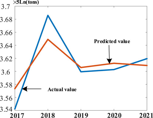
FIGURE 6. Region J carbon emission prediction results, 2017–2021.

Compared with the true carbon emissions value obtained through the carbon emission calculation method in the IPCC guideline, the prediction error of the proposed prediction model in this paper is 1.05%, which verifies the effectiveness and feasibility of the proposed carbon emission prediction method in urban areas.

4.3 Calculation based on the GIOWA combination prediction

The GIOWA combination method has high flexibility and adaptability. The partial weights can be adjusted and reconfigured according to the requirements. The weight is adjusted according to the prediction results and the degree of error to maintain the effectiveness and adaptability of the predicted carbon emission portfolio. The micro-forecast is based on energy consumption data, such as enterprise-level electricity consumption, while the macro-forecast is based on the regional economy and population. There are differences between the two benchmarks and nonlinear links. The GIOWA combination prediction method is used to achieve a more accurate prediction of regional carbon emissions.

The initial weight of the micro-forecast data and macro-prediction is set according to the degree of error between micro- and macro-data. Therefore, the initial weight for the micro-forecast ratio is 0.75, and the macro-layer ratio is 0.25. Based on Eqs 13–15, the GIOWA combination prediction is shown in Figure 7 shows the result of calculating the GIOWA combination and comparing the microscopic and macroscopic prediction curves.

FIGURE 7

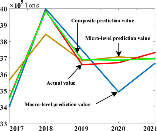
FIGURE 7. Three forecasts and actual carbon emission results.

The prediction effect of the combined prediction value is much better than that of the micro-prediction effect and the macro-prediction. The errors for each prediction are shown in Table 4.

TABLE 4

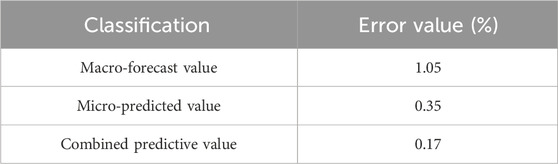
TABLE 4. Three categories of prediction and their error values.

Compared with the macro-prediction error, the combined prediction is reduced by 0.88%, improving the accuracy of 83.81%, reducing the micro-prediction error by 0.185%, and improving the accuracy of 52.11%. The feasibility and validity of the combined prediction are verified.

The initial weight of the combined prediction will be updated in real time, based on the historical data. The micro-prediction and macro-prediction error will not always be constant. With 5 years as a sample set, each year should update the micro- and macro-prediction method and calculate the corresponding error value. Selecting the smallest error value prediction method and obtaining the prediction value, through the error value comparison combination prediction initial weight, enables the reduction of the prediction error.

5 Conclusion

Considering the limited carbon emission calculation data in the regional areas of most cities, the regional carbon emission generalization is weak when calculating using the carbon emission accounting method in the IPCC guidelines. The method discussed here considers the forecast of urban regional combined carbon emissions based on micro-enterprise electricity consumption data and macro-regional data. The empirical analysis is based on a state-level new district of an eastern city, and the main conclusions are given as follows:

By calculating the DTW value of power carbon emissions in various industries and regions, it is found that the total carbon emission of manufacturing, wholesale and retail, construction, housing, and transportation accounts for approximately 87% of the total power carbon emission of a key city in eastern China, which is the main carbon emission source of region J. Compared with the true carbon emission value calculated by the IPCC carbon emission accounting model, the test average error in the proposed regional carbon emission prediction model is 0.53%, and the prediction error is 0.35%, which verifies the feasibility of the microscopic prediction model.

Using the STIRPAT model to analyze the factors influencing region J carbon emissions, maintaining the slow growth of the economy and population, and reducing the proportion of the energy consumption of high-carbon emission industries in the whole city can effectively reduce the regional carbon emissions, which, at the same time, reduces the proportion of energy consumption in the city of high energy consumption and high-carbon emission industries in the city and increases the proportion of low carbon emissions and low-energy consumption enterprises. Compared with the true carbon emission value calculated by the IPCC carbon emission accounting model, the proposed carbon emission prediction error based on the STIRPAT model is 1.05%, which verifies the feasibility of the macroscopic prediction model.

The prediction error value can be greatly reduced. In addition, the error value of the micro-prediction value and the macro-prediction value is used as the preset initial weight reference of the GIOWA combination, and the combined prediction is made. The prediction error is reduced to 0.17%, which is far lower than the error value of the micro-prediction model and macro-prediction model, which further verifies the feasibility of the combined prediction model.

There are still the following shortcomings in this study:

There is limited sample data and a single source of data. Therefore, in subsequent research studies, the collection methods of data will be further expanded, and the same data from different sources will be screened and screened again. An increase in the regional case analysis and select regions with different geographical conditions for research and analysis at the geographical level will be seen. At the climate level, we will classify and predict the four seasons of spring, summer, autumn, and winter and will further refine the data scale.

This study has a lack of algorithm comparison experiments. In the subsequent research process, other carbon emission prediction methods will be selected for comparisons, and a more comprehensive comparative analysis will be conducted from the aspects of the error rate, robustness, etc., in order to obtain the best prediction results.

Data availability statement

The original contributions presented in the study are included in the article/Supplementary Material; further inquiries can be directed to the corresponding author.

Author contributions

HZ: writing–original draft. FQ: writing–review and editing. CL: writing–review and editing. GL: writing–review and editing. GX: writing–review and editing.

Funding

The author(s) declare that financial support was received for the research, authorship, and/or publication of this article. This work is supported by the State Grid Corporation of China (No. J2022163, the Key Science and Technology Project of State Grid Jiangsu Electric Power Co.).

Conflict of interest

Authors HZ, FQ, CL, GL, and GX were employed by State Grid Jiangsu Electric Power Co., Ltd.

Publisher’s note

All claims expressed in this article are solely those of the authors and do not necessarily represent those of their affiliated organizations, or those of the publisher, the editors, and the reviewers. Any product that may be evaluated in this article, or claim that may be made by its manufacturer, is not guaranteed or endorsed by the publisher.

References

Cao, Y., Zhou, B., Chung, C. Y., Shuai, Z., Hua, Z., Sun, Y., et al. (2022). Dynamic modelling and mutual coordination of electricity and watershed networks for spatiotemporal operational flexibility enhancement under rainy climates. IEEE transactions on smart grid. doi:10.1109/T5G.2022.3223877

CrossRef Full Text | Google Scholar

Cheng, J., Huang, C., Gan, X., Peng, C., and Deng, L. (2023). Can forest carbon sequestration offset industrial CO2 emissions? A case study of Hubei Province, China. J. Clean. Prod. 426, 139147. doi:10.1016/j.jclepro.2023.139147

CrossRef Full Text | Google Scholar

Deng, J., Jiang, F., Wang, W., He, G., Zhang, X., Liu, K., et al. (2022). Low-carbon Optimized Operation ofIntegrated Energy SystemConsidering Electric heat Flexible Load and HydrogenEnergy Refined Modeling [J]. Power System Technology 46 (5), 1692–1702. doi:10.13335/j.1000-3673.pst.2021.1373

CrossRef Full Text | Google Scholar

Hosseini, S. M., Saifoddin, A., Shirmo, H. R., and Aslani, A. (2019). Forecasting of CO2 emissions in Iran based on time series and regression analysis. Energy Rep. 5, 619–631. doi:10.1016/j.egyr.2019.05.004

CrossRef Full Text | Google Scholar

Jiang, F., Lin, Z., Wang, W., Wang, X., Xi, Z., Guo, Q., et al. (2023). Optimal Bagging ensemble ultra short tern multivariate load forecasting considering minimum average envelope entropy load decomposition. Proc. CSEE, 1–17. doi:10.13334/j.0258-8013.pcsee.223470

CrossRef Full Text | Google Scholar

Jiang, F., Peng, X., Tu, C., Guo, Q., Deng, J., and Dai, F. (2021). An improved hybrid parallel compensator for enhancing PV power transfer capability. IEEE Trans. industrial Electron. 69 (11), 11132–11143. doi:10.1109/tie.2021.3121694

CrossRef Full Text | Google Scholar

Karlsson, I., Rootzén, J., and Johnsson, F. (2020). Reaching net-zero carbon emissions in construction supply chains–Analysis of a Swedish road construction project. Renew. Sustain. Energy Rev. 120, 109651. doi:10.1016/j.rser.2019.109651

CrossRef Full Text | Google Scholar

Li, G., Chen, X., and You, X. (2023). System dynamics prediction and development path optimization of regional carbon emissions: a case study of Tianjin. Renew. Sustain. Energy Rev. 184, 113579. doi:10.1016/j.rser.2023.113579

CrossRef Full Text | Google Scholar

Li, Y., and Wang, Q. (2019). Exploring carbon emissions in China's electric power industry for low carbon development: drivers, decoupling analysis and policy implications. Pol. J. Environ. Stud. 28 (5), 3353–3367. doi:10.15244/pjoes/93929

CrossRef Full Text | Google Scholar

Li, Y., Zhang, N., Du, E., Liu, Y., Cai, X., He, D., et al. (2022). Research on the low-carbon demand response mechanism and benefit analysis of power systems based on carbon emissions. Proc. CSEE 42 (08), 2830–2842. doi:10.13334/1.0258-8013.pcsee.220308

CrossRef Full Text | Google Scholar

Liu, Z., Sun, T., Yu, Y., Ke, P., Deng, Z., Lu, C., et al. (2022). Near-real-time carbon emission accounting technology toward carbon neutrality. Engineering 14, 44–51. doi:10.1016/j.eng.2021.12.019

CrossRef Full Text | Google Scholar

Liu, Z., Wang, C., Li, P., Yu, H., Yu, L., Li, P., et al. (2021). State estimation of distribution networks based on multi-source measurement data and its applications. Proc. CSEE 41 (8), 2605–2614. doi:10.13334/j.0258-8013.pcsee.201416

CrossRef Full Text | Google Scholar

Luo, Y., Li, Z., Li, S., and Jiang, F. (2023a). Risk assessment for energy stations based on real-time equipment failure rates and security boundaries. Sustainability 15 (18), 13741. doi:10.3390/su151813741

CrossRef Full Text | Google Scholar

Luo, Y., Jiang, F., Sun, M., Guo, G., and Zeng, Z. (2023b). Dynamic evaluation of health state vector of distributed energy stations based on prospect theory and reference value transformation. Power Syst. Technol. 47 (11), 4438–4447.

Google Scholar

Nie, H., and Kemp, R. (2014). Index decomposition analysis of residential energy consumption in China: 2002 - 2010. Appl. Energy 121, 10–19. doi:10.1016/j.apenergy.2014.01.070

CrossRef Full Text | Google Scholar

Ofosu, A. J., Xie, N. M., and Javed, S. A. (2020). Forecasting CO2 emissions of China's cement industry using a hybrid Verhulst-GM(1, N) model and emissions technical conversion. Renew. Sustain. Energy Rev. 130, 109945. doi:10.1016/j.rser.2020.109945

CrossRef Full Text | Google Scholar

Peng, Y., Yang, Y., Chen, M., Wang, X., Xiong, Y., Wang, M., et al. (2023). Value evaluation method for pumped storage in the new power system. Chin. J. Electr. Eng. 9 (3), 26–38. doi:10.23919/cjee.2023.000029

CrossRef Full Text | Google Scholar

Shi, Q., Zheng, B., Zheng, Y., Tong, D., Liu, Y., Ma, H., et al. (2022). Co-benefits of CO2 emission reduction from China’s clean air actions between 2013-2020. Nat. Commun. 13 (1), 5061. doi:10.1038/s41467-022-32656-8

PubMed Abstract | CrossRef Full Text | Google Scholar

Wang, Y., and Zhao, T. (2018). Panel estimation for the impacts of residential characteristic factors on CO2 emissions from residential sector in China. Atmos. Pollut. Res. 9 (4), 595–606. doi:10.1016/j.apr.2017.12.010

CrossRef Full Text | Google Scholar

Yi, C. Y., Gwak, H. S., and Lee, D. E. (2017). Stochastic carbon emission estimation method for construction operation. J. Civ. Eng. Manag. 23 (1), 137–149. doi:10.3846/13923730.2014.992466

CrossRef Full Text | Google Scholar

Zhang, H., Sun, W., Li, W., and Ma, G. (2022). A carbon flow tracing and carbon accounting method for exploring CO2 emissions of the iron and steel industry: an integrated material–energy–carbon hub. Appl. Energy 309, 118485. doi:10.1016/j.apenergy.2021.118485

CrossRef Full Text | Google Scholar