Water level control of nuclear steam generators using intelligent hierarchical autonomous controller

The challenge of water level control in steam generators, particularly at low power levels, has always been a critical aspect of nuclear power plant operation. To address this issue, this paper introduces an IHA controller. This controller employs a CPI controller as the primary controller for direct water level control, coupled with an agent-based controller optimized through a DRL algorithm. The agent dynamically optimizes the parameters of the CPI controller in real-time based on the system’s state, resulting in improved control performance. Firstly, a new observer information is obtained to get the accurate state of the system, and a new reward function is constructed to evaluate the status of the system and guide the agent’s learning process. Secondly, a deep ResNet with good generalization performance is used as the approximator of action value function and policy function. Then, the DDPG algorithm is used to train the agent-based controller, and an advanced controller with good performance is obtained after training. Finally, the popular UTSG model is used to verify the effectiveness of the algorithm. The results demonstrate that the proposed method achieves rise times of 73.9 s, 13.6 s, and 16.4 s at low, medium, and high power levels, respectively. Particularly, at low power levels, the IHA controller can restore the water level to its normal state within 200 s. These performances surpass those of the comparative methods, indicating that the proposed method excels not only in water level tracking but also in anti-interference capabilities. In essence, the IHA controller can autonomously learn the control strategy and reduce its reliance on the expert system, achieving true autonomous control and delivering excellent control performance.

1 Introduction

A typical natural circulation steam generator takes the form of a vertical, UTSG, as depicted in Figure 1. This configuration serves as a critical component within the primary coolant system of a nuclear reactor. Its primary purpose is to function as a heat exchanger, facilitating the transfer of heat extracted from the reactor’s primary coolant to a secondary fluid via a bundle of heat transfer tubes (Sui et al., 2020). This heat exchange process generates saturated steam, which is subsequently conveyed to a steam turbine for electricity generation. Moreover, the steam generator assumes a pivotal role in linking the primary and secondary coolant loops and acts as a safety barrier to prevent the release of radioactive materials. To ensure the safe operation of the UTSG, it is imperative to maintain the water level within a defined range. If the water level becomes excessively low, it can lead to damage to the heat transfer tubes. Conversely, an excessively high water level can impact the steam-water separation process, resulting in a decline in steam quality and potential damage to the steam turbine (Kong et al., 2022). Therefore, any abnormal water level conditions in the UTSG necessitate a shutdown, which can have adverse consequences on the economic and safety aspects of PWRs.

FIGURE 1

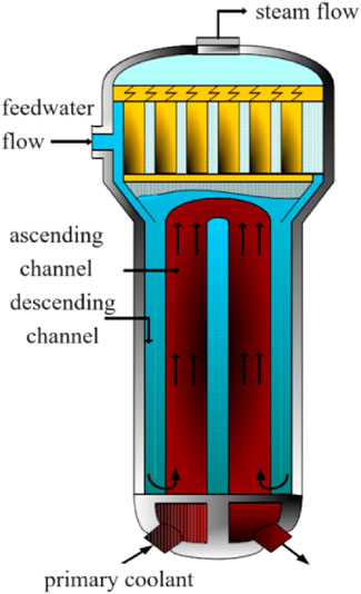
FIGURE 1. Steam generator structure diagram.

UTSG has “shrink and swell” effects during operation, making it a complex system with non-linear and non-minimum phases, and has a small stability margin, which brings many difficulties to the controller design. In order to solve the UTSG water level control problem, the researchers have done a lot of valuable work in this area. Wan et al. (Wan et al., 2017), Rao et al. (Rao et al., 2024), Safarzadeh et al. (Safarzadeh et al., 2011) and Irving et al. (Irving et al., 1980) respectively proposed UTSG mathematical models that can accurately reflect the characteristics of the water level. Among them, the model proposed by Irving covers a variety of power level conditions, so it is widely used in control algorithm research, and this model was also used for our control algorithm research. The CPI controller can mitigate the influence of “shrink and swell” effects to some extent. By utilizing the actual measured water level signal, it undergoes a first-order inertia stage, causing transient signals during water level expansion to be delayed. This delay allows the deviation signal between steam flow and feedwater flow to increase the feedwater amount, thus achieving the correct action. On the other hand, it takes advantage of the characteristic that the flow error output by the water level control unit and the trend of steam flow change in the opposite direction. This characteristic is employed to eliminate the impact of “shrink and swell” effects. Consequently, the CPI controller remains widely employed in the water level control system of UTSG.

In order to achieve robust stability and optimal dynamic performance, it is necessary to tune the parameters of the PID controller. Online self-tuning methods for PID control parameters possess the capabilities of self-learning, adaptability, and self-organization. They can dynamically adjust the PID model parameters online, adapting to the continuous changes in the object model parameters. So far, researchers have conducted a substantial amount of intriguing studies in this area. The Expert PID control method combines control experience patterns from an expert knowledge base, deriving the parameters of the PID controller through logical reasoning mechanisms. However, it heavily relies on the expert’s experience, and the proficiency of the expert determines the effectiveness of the controller (Hu and Liu, 2020; Xu and Li, 2020). The Fuzzy PID control method condenses empirical knowledge into a fuzzy rule model, achieving self-tuning of PID parameters through fuzzy reasoning. It similarly depends on human experience, with the configuration of membership functions for process variables having a significant impact on the system (Li et al., 2017; Maghfiroh et al., 2022; Zhu et al., 2022). The Neural Network PID control method utilizes the nonlinear approximation capability of neural networks, dynamically adjusting PID parameters based on the system’s input and output data to optimize control performance. However, it faces challenges such as acquiring training data and susceptibility to local optima (Rodriguez-Abreo et al., 2021; Zhang et al., 2022). The Genetic PID control method simulates the process of natural selection and genetic mechanisms to optimize controller parameters for improved control performance. It does not require complete information about the controlled object, but it has drawbacks like high computational demands and slow convergence speed (Zhou et al., 2019; Ahmmed et al., 2020).

To overcome the limitations of the aforementioned optimization algorithms, we explore the application of DRL algorithm, specifically DDPG, in the water level control of the UTSG. DDPG empowers agents with the capability for self-supervised learning, enabling them to interact autonomously with the environment, make continuous progress through trial and error, and collect training samples stored in an experience replay buffer. This helps reduce the correlation among samples and enhances training stability, all while decreasing the reliance on expert knowledge (Wang and Hong, 2020). DDPG employs an Actor-Critic structure, where the Actor network is responsible for policy generation, and the Critic network estimates state values or state-action values. These two networks collaborate in learning to improve performance. DDPG offers higher sample efficiency, implying that it can learn good policies in relatively few training steps without requiring extensive computational resources.

To achieve real-time optimization of PI controller parameters and reduce the difficulty of controller design, an IHA controller is proposed. The proposed controller uses the CPI controller as a primary controller and introduces DRL to build an advanced agent-based controller with autonomous control capabilities, which can continuously improve the CPI control strategy according to the state of the environment. The main contributions and innovation of this paper are as follows:

(1) A new reward function is proposed to improve the training effect of the model.

(2) The DDPG algorithm is used to optimize the agent-based controller, which can learn the control strategy independently.

(3) The deep ResNet is used as approximators of action-value and action functions to obtain better generalization performance.

(4) The UTSG water level model is used to verify the effectiveness of the proposed method.

The remainder of this paper is organized as follows. In Section 2 we present methods. We then present in detail the UTSG model and controller structure in Section 3. The experimental test case results and discussions are provided in Section 4. Finally, Section 5 concludes the paper.

2 Methods

2.1 Reinforcement learning

RL is an important branch of machine learning (Carapuço et al., 2018), but unlike supervised learning and unsupervised learning, it is an active learning process, which does not require specific training data, and agents need to obtain samples in the process of continuous interaction with the environment. As shown in Figure 2, by taking the goal of maximizing the cumulative reward, RL continuously optimizes the strategy based on the state, action, reward and other information, and finally finds the optimal state-action sequence during the training process. The process is very similar to that of human learning, in which strategies are continually improved through interaction and trial and error with the environment.

FIGURE 2

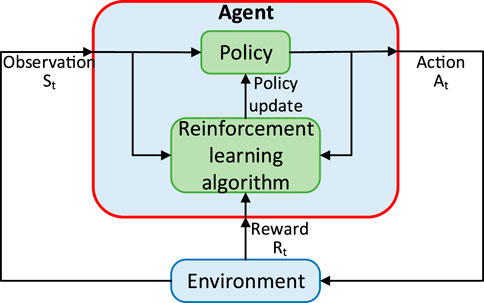
FIGURE 2. The work procession of RL.

The interactive process can be expressed by Markov decision processes (Bi et al., 2019). Suppose the environment is completely observable, the state space of the environment is represented by S, and the action space is represented by A; the behavior of the agent is defined by policy π, which defines a probability distribution p(A) to represent the relationship between state and action. At time t, let $s_t\left(s_t\in \mathit{S}\right)$ be the state of the environment, and $a_t$ ($a_t\in \mathbf{A}$) be the action taken by the agent according to the state $s_t$ and then at time t+1, the state transitions to $s_{t+1}$. In this process, the instant reward received by the agent can be expressed as $r\left(s_t,a_t\right)$. For the entire process $t=1,2,3,\dots ,T$, the historical state information can be represented by state-action pairs ${\mathrm{s}}_{\mathrm{t}}=\left(s_1,a_1,\dots ,{s_{t-1},a}_{t-1}\right)$. The sum of discounted future reward returned $R_t$ by the agent after performing the action $a_t$ is defined as

$R_t={\displaystyle {\sum }_{i=t}^T}{\gamma }^{i-t}r\left({\mathrm{s}}_i,a_i\right)(1)$

Where $\gamma$ is the discounting factor, and $\gamma \in \left[0,1\right]$. It can be found that $R_t$ has a great relationship with the action selected by the policy, and RL is to learn the optimal policy to maximize the expected return from the start distribution $J=E_{r_i,s_i\sim E,a_i\sim \pi }\left[R_1\right]$. We represent the discounted state access distribution of policy π as ${\rho }^{\pi }$.

In order to describe the expected return of the model under the state ${\mathrm{s}}_{\mathrm{t}}$, the action $a_t$ taken by the agent, and under the guidance of the policy π, an action-value function $Q^{\pi }\left(s_t,a_t\right)$ is used to express it (Sutton et al., 2000), which is defined as

$Q^{\pi }\left(s_t,a_t\right)=E_{r_{i\ge t},s_{i\ge t}\sim E,a_{i\ge t}\sim \pi }\left[R_t|s_t,a_t\right](2)$

The above formula can be converted into a recursive form through the Bellman equation as:

$Q^{\pi }\left(s_t,a_t\right)=E_{r_t,s_{t+1}\sim E}\left[r\left(s_t,a_t\right)+\gamma {\mathbb{E}}_{a_{t+1^{\sim \pi }}}\left[Q^{\pi }\left(s_{t+1},a_{t+1}\right)\right]\right](3)$

2.2 Deep deterministic policy gradient

DDPG is a model-free DRL method based on the critic-actor framework and deterministic policy gradient algorithm (Lillic et al., 2016; Thomas and Brunskill, 2017). In the processing of high-dimensional state space and action space, DDPG uses deep neural networks (Sen Peng et al., 2018) as the approximator of action function and action-value function, which also brings a problem. The training process of the neural network needs to assume that the samples follow an independent distribution, but the samples obtained in chronological order obviously do not meet this requirement. To solve this problem, DDPG draws on the experience replay mechanism in deep Q-network (Mnih et al., 2015) and the minibatch training method in deep neural networks to ensure the stability of the training process of large-scale nonlinear networks.

To avoid the inner expectation of the deterministic policy, the deterministic policy function $\mu :\mathit{S}\leftarrow \mathit{A}$ is used to describe the action-value function:

$Q^{\mu }\left({\mathrm{s}}_t,a_t\right)=E_{r_t,s_{t+1}\sim E}\left[r\left(s_t,a_t\right)+\gamma Q^{\mu }\left(s_{t+1},\mu \left(s_{t+1}\right)\right)\right](4)$

2.2.1 Experience replay mechanism

In continuous control tasks, samples are usually collected in chronological order, and the data are highly correlated, so the variance between samples is small, which is obviously not conducive to the training of agents. Experience replay is used to solve this problem (Mnih et al., 2015), and a fixed-size replay buffer is created to cache the collected data. The data collected during each task execution process will be stored in the replay buffer in tuple $\left(s_t,a_t,r_t,s_{t+1}\right)$. During each training, a minibatch of samples are randomly selected from the replay buffer, which can reduce the correlation between the data and improve training efficiency.

2.2.2 Policy exploration

Policy exploration is a very important part in RL, which is used to explore unknown policies. If the explored policies are superior to the current policies, they can play an evolutionary role for the policies. In order to solve the exploration problem in continuous control tasks, the exploration policy ${\mu }^{\prime }$ is constructed by adding noise to the policy $\mu$:

${\mu }^{\prime }\left(s_t\right)=\mu \left(s_t|{\theta }_t^{\mu }\right)+N(5)$

Where $N$ is the actor noise. Considering that the plant used in this paper is an inertial system, Ornstein-Uhlenbeck process (Uhlenbeck and Ornstein, 1930) is used to generate time-related noise sequences to improve the exploration efficiency of control tasks in the inertial system. Ornstein-Uhlenbeck process is a random process, and its discrete form is

$x\left(t\right)=x\left(t-1\right)+a\left(\delta -x\left(t-1\right)\right)T_s+\sigma ϵ\sqrt{T_s}(6)$

Where $\delta$ and $\sigma$ are the mean and variance of the noise model, $ϵ$ is a random number, $a$ is a constant, which determines the speed at which the noise model output approaches the mean, and $T_s$ is the sampling time.

2.2.3 Function approximators

In order for the agent to learn a better control strategy, it is very vital to select an appropriate function approximators. Considering that the deep neural network has strong adaptability, it can approximate any function in a nonlinear form, so it is also the most used function approximator. We use deep ResNet (He et al., 2016) as a function approximator, which is constructed with residual structure, shown in Figure 3A. The critic network (Figure 3B) and action network (Figure 3C) are constructed for the value function and action function, respectively. The activation function of the hidden layer of the network approximator is the linear rectification function and the activation function of the output layer is the tanh function.

FIGURE 3

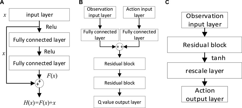
FIGURE 3. Network structure. (A) ResNet structure; (B) Critic network structure; (C) Actor network structure.

2.2.4 Training process

In this paper, the critic network, actor network, target critic network and target actor network are defined as $Q\left(s,a|{\theta }^Q\right)$, $\mu \left(\left.s\right|{\theta }^{\mu }\right)$, $Q^{\prime }\left(s,a|{\theta }^{Q^{\prime }}\right)$ and ${\mu }^{\prime }\left(\left.s\right|{\theta }^{{\mu }^{\prime }}\right)$ respectively, where ${\theta }^Q$, ${\theta }^{\mu }$, ${\theta }^{Q^{\prime }}$ and ${\theta }^{{\mu }^{\prime }}$ are the parameters of each approximator. The main network and the target network have the same network structure, which is defined in Section 2.2.3.

The pseudocode of the DDPG algorithm is shown in Table 1. During the training process, the network needs to be updated at every timestep. To ensure a stable training process, the network is trained using a minibatch training method. Suppose that each time N samples are taken from the replay buffer to form the training set $R$. During the training process, the critic network is optimized by minimizing the loss function:

$L\left({\theta }^Q\right)=\frac{1}{N}{\displaystyle {\sum }_i}{\left(y_i-Q\left(s_i,a_i|{\theta }^Q\right)\right)}^2(7)$

where

$y_i=r_i+\gamma Q^{\prime }\left(s_{i+1},{\mu }^{\prime }\left(s_{i+1}|{\theta }^{{\mu }^{\prime }}\right)|{\theta }^{Q^{\prime }}\right)(8)$

TABLE 1

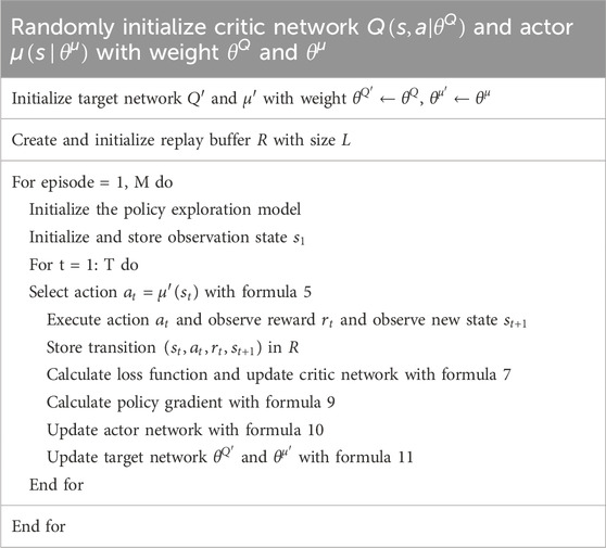
TABLE 1. DDPG algorithm.

The start distribution $J$ with respect to the actor parameters can be obtained by the following formula:

${\nabla }_{{\theta }^{\mu }}J\approx \frac{1}{N}{\displaystyle {\sum }_i}{\nabla }_{a}Q\left(\left.s,a\right|{\theta }^Q\right){|}_{s=s_t,a=\mu \left(s_i\right)}{\nabla }_{{\theta }^{\mu }}\mu \left(\left.s\right|{\theta }^{\mu }\right){|}_{s=s_i}(9)$

Then use gradient ${\nabla }_{{\theta }^{\mu }}J$ to update the action network:

${\theta }_i^{\mu }={\theta }_i^{\mu }+{\alpha }^{\mu }{\nabla }_{{\theta }^{\mu }}J(10)$

Finally, use the soft update method to update the parameters of the target network ${\mathrm{Q}}^{\prime }\left(\left.\mathrm{s},\mathrm{a}\right|{\mathrm{\theta }}^{Q^{\prime }}\right)$ and ${\mathrm{\mu }}^{\prime }\left(\left.s\right|{\theta }^{{\mu }^{\prime }}\right)$:

${\theta }^{Q^{\prime }}=\eta {\theta }^Q+\left(1-\eta \right){\theta }^{Q^{\prime }}(\mathrm{11a})$

${\theta }^{{\mu }^{\prime }}=\eta {\theta }^{\mu }+\left(1-\eta \right){\theta }^{{\mu }^{\prime }}(\mathrm{11b})$

where $\eta \ll 1$, which makes the update speed of the target network very slow, thereby greatly improving the robustness of the learning process.

3 UTSG control model

3.1 Mathematical model

An adept UTSG model is crucial for the design and testing of control algorithms. Typically, thermal-hydraulic models based on conservation principles of mass, energy, and momentum are employed to precisely simulate the operational characteristics of steam generators. However, such models often exhibit intricate non-linear features, posing challenges in controller design. In practice, a UTSG model that is relatively straightforward yet accurate, faithfully capturing dynamic traits, is preferred. The linear model proposed by Irving (Irving et al., 1980), derived through a fusion of experimental and theoretical approaches, has undergone rigorous validation across multiple power levels, affirming its precision in replicating operational characteristics. Consequently, it has found extensive application in the realm of control algorithm research. This model establishes a transfer function model related to feed water flow $Q_e$, steam flow $Q_v$ and narrow-range water level $Y$:

$Y\left(s\right)=\frac{G_1}{s}\left[Q_e\left(s\right)-Q_v\left(s\right)\right]-\frac{G_2}{1+{\tau }_{2}s}\left[Q_e\left(s\right)-Q_v\left(s\right)\right]+\frac{G_{3}s}{s^2+2{\tau }_1^{-1}+{\tau }_1^{-2}+4{\pi }^2{T}^{-2}}{Q}_e\left(s\right)(12)$

Where $s$ is Laplace variable, $G_1$, $G_2$ and $G_3$ are constant, ${\tau }_2$ is the delay time of the shrink and swell phenomenon, ${\tau }_1$ is the delay time of the mechanical oscillation, and $T$ is the period of the mechanical oscillation. The first term $X_1\left(s\right)=\frac{G_1}{s}\left[Q_e\left(s\right)-Q_v\left(s\right)\right]$ calculates the change in water level by summing the flow in and out, which represents the wide-ranging effect of UTSG. The second term $X_2\left(s\right)=\frac{G_2}{1+{\tau }_{2}s}\left[Q_e\left(s\right)-Q_v\left(s\right)\right]$ is used to describe the inverse kinetic phenomena caused by shrink and swell effects. The third term $X_3\left(s\right)=\frac{G_{3}s}{s^2+2{\tau }_1^{-1}+{\tau }_1^{-2}+4{\pi }^2{T}^{-2}}{Q}_e\left(s\right)$ represents the effect of water level oscillations generated by the feed water in the annular descending channel. The values of the power-related parameters of this model at 5 typical power levels are given in Table 2.

TABLE 2

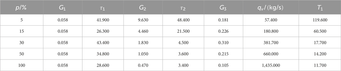
TABLE 2. The UTSG model parameters in different power level.

3.2 Model dynamic characteristics analysis

In order to understand the dynamic characteristics of the model, this section will briefly analyze the response characteristics of the model when the feed water flow and steam flow step +1 kg/s respectively in conjunction with the shrink and swell phenomenon.

When the feedwater flow rate experiences a step increase of +1 kg/s, the corresponding dynamic response of the UTSG water level is illustrated in Figure 4A. It becomes evident that the initial surge in feedwater flow prompts a surge in water level, irrespective of the power levels. Subsequently, as the feedwater temperature falls below the saturation temperature, leading to an augmentation in subcooling within the bundle and consequent steam condensation, the water level descends. Given that the feedwater flow surpasses the steam flow, the water level sustains an upward trajectory, a phenomenon colloquially referred to as the ‘shrink effect’.

FIGURE 4

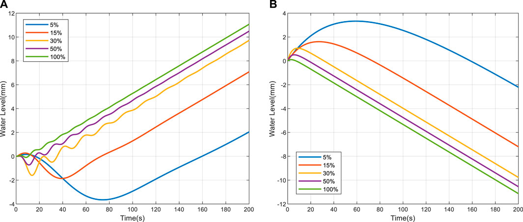
FIGURE 4. Water level response. (A) When the feed water flow steps 1 kg/s; (B) When the steam flow steps 1 kg/s.

When a step increase of +1 kg/s in steam flow is applied, the associated dynamic response of the UTSG water level is depicted in Figure 4B. It becomes evident that, across varying power levels, as steam flow escalates, the pressure within the steam dome diminishes, leading to a reduction in the saturation temperature of the water and an augmentation in boiling within the bundle area. Consequently, the water level initially experiences an ascent. As the steam flow surpasses that of the feedwater, a sustained decline in the water level ensues, a phenomenon commonly referred to as the ‘swell effect’.

Simultaneously, it is noteworthy that, for distinct power levels, identical disturbances in feedwater flow or steam flow yield varying degrees of both the shrink and swell effects. Additionally, it is observed that the transition time during low-power operations exceeds that observed during high-power conditions. This phenomenon underscores the inherent challenges in regulating water levels within the low-power range.

3.3 Cascaded PI controller

Compared with single control loop, the cascaded control is more controllable and safer, and has better robustness (Jia et al., 2020). Therefore, CPI controller is adopted as the basic controller in this paper. The working process of CPI controller is shown in Figure 8. In the outer loop control, the difference between the expected water level and the model output water level is used as the input of the controller. Its function is mainly used to control the water level to track the change of the expected value. In the inner loop control, the sum of the output of the outer loop controller and the steam flow rate minus the feed water flow is used as the input of the controller, which is mainly used to suppress the steam flow disturbance.

The working principle of PI controller is expressed as:

$u\left(t\right)=Kp\left(e\left(t\right)+Ki{\int }_0^{t}e\left(t\right)dt\right)(13)$

Where $e\left(t\right)$ is the error, $Kp$ is the proportional coefficient, and $Ki$ is the integral coefficient; in this paper, the proportional and integral coefficients of the outer loop controller are defined as $Kp1$, $Ki1$, and the corresponding parameters of the inner loop controller are defined as $Kp2$, $Ki2$.

3.4 Controller design

The IHA controller proposed in this paper uses a double level controller structure, shown in Figure 5. The CPI controller is used as primary controller, which is responsible for directly controlling the water level of the UTSG model; the advanced controller uses an agent-based controller with intelligent characteristics, which is responsible for online adjustment of the parameters of the CPI controller. In control process, the primary controller and the advanced controller work together to adjust the control policy in real time according to the state of the system and realize intelligent autonomous control.

FIGURE 5

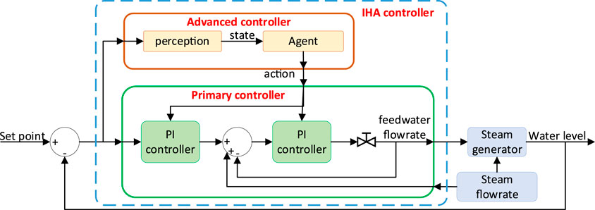
FIGURE 5. UTSG water level control process.

3.5 Observer information

The accurate observer information should be provided to represent the dynamic characteristics of the controlled object. In the controller system, the error and the reciprocal of error are often used to indicate the state of the system, which is more suitable for single-target control. However, the UTSG needs to change between different water levels, and various system states need to be considered using the above state expression. To improve this phenomenon, the relative error and reciprocal of relative error are used to represent the state of system. In this way, different target control can be achieved by designing only one state representation, which greatly simplifies the complexity. At the same time, this paper draws on the ideas of (Mnih et al., 2015). In continuous control tasks, the continuous-time environmental state is related, and the observed variable for a period is embraced as the environmental state representation, which can more accurately reflect the state of the system.

In this paper, the values of relative error $re\left(t\right)$ and reciprocal $\frac{\partial re\left(\mathrm{t}\right)}{\partial t}$ in consecutive 3s are used as observer information to obtain the observer vector ${\mathit{s}}_1\left(t\right)$ of the error term and the observation vector ${\mathit{s}}_2\left(t\right)$ of the reciprocal term, which are defined as follows:

${\mathit{s}}_1\left(t\right)=\left\{\begin{array}{c}{w_1\left[0,0,re\left(t\right)\right]}^{\mathrm{T}},t=0\\ {w_1\left[0,re\left(t-1\right),re\left(t\right)\right]}^{\mathrm{T}},t=1\\ {w_1\left[re\left(t-2\right),re\left(t-1\right),re\left(t\right)\right]}^{\mathrm{T}},t\ge 2\end{array}\right.(\mathrm{14a})$

${\mathit{s}}_2\left(t\right)=\left\{\begin{array}{c}{w_2\left[0,0,\frac{\partial re\left(t\right)}{\partial t}\right]}^{\mathrm{T}},t=0\\ {w_2\left[0,\frac{\partial re\left(t-1\right)}{\partial t},\frac{\partial re\left(t\right)}{\partial t}\right]}^{\mathrm{T}},t=1\\ {w_2\left[\frac{\partial re\left(t-2\right)}{\partial t},\frac{\partial re\left(t-1\right)}{\partial t},\frac{\partial re\left(t\right)}{\partial t}\right]}^{\mathrm{T}},t\ge 2\end{array}\right.(\mathrm{14b})$

$re\left(t\right)=\frac{ta-y\left(t\right)}{ta}(\mathrm{14c})$

where $ta$ is the target value, $w_1$ and $w_2$ are normalization coefficients, which is used to transform the value to the interval [0,1], to promote the training efficiency of the neural network. At time $t=0$, $e\left(t\right)=\frac{\partial re\left(t\right)}{\partial t}=0$. Finally, the observation vectors ${\mathit{s}}_1\left(t\right)$ and ${\mathit{s}}_2\left(t\right)$ are combined to obtain a comprehensive observation matrix $\mathit{s}\left(t\right)$ with a dimension of 3 × 2:

$\mathit{s}\left(t\right)=\left[{\mathit{s}}_1\left(t\right),{\mathit{s}}_2\left(t\right)\right](15)$

Therefore, the dimension of observer information is determined to be 3 × 2, and the dimension of action information is determined to be 4 × 1. The network structure of action network and critic network is further confirmed, as shown in Table 3.

TABLE 3

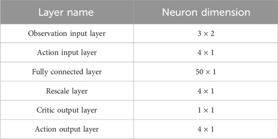
TABLE 3. The number of neurons in different layers.

3.6 Reward function

The reward function can also be called the evaluation function. A good reward function not only speeds up the learning process, but also makes it easier to find the global optimal solution. The commonly used evaluation functions are ITAE, ITSE and integral of squared time weighted errors. However, these functions are suitable for evaluating the entire control process. In the RL process, the control effect of each step needs to be evaluated, and it has a strong guiding effect on the learning process. Therefore, a new evaluation function is needed to evaluate the learning process.

In fact, in the control process, when the water level error is large, the PI controller needs a large gain to obtain a large response speed, and when the error is small, the value of the gain needs to be reduced to avoid overshoot. Therefore, this paper constructs a segmented evaluation function $r\left(t\right)$, which can guide the learning process by adjusting some parameters. Experiments show that this function can quickly and effectively guide the agent’s learning, which will be introduced below.

According to the difference in absolute value of relative error $\left|re\left(t\right)\right|$, we specifies that $\left|re\left(t\right)\right|>200\%$ is the abnormal area, $200\%\ge \left|re\left(t\right)\right|>15\%$ is the large error area, and $\left|re\left(t\right)\right|\le 15\%$ is the low error area.

Within the abnormal region, where the system strays significantly from the target value, a proactive approach is adopted. The ongoing task is promptly terminated, and a fresh training process is initiated to conserve valuable training time. Simultaneously, a correspondingly modest reward value is prescribed to guide the agent away from this undesirable state. In contrast, the expansive error zone warrants a heightened emphasis on speed of response, with the overarching goal being swifter rectification without excessive deliberation. Consequently, when the relative error resides within this territory, the reward value is uniformly designated as −2. Within the realm of low error, where the system’s output closely approximates the desired value but is susceptible to overshooting and necessitates prolonged adjustment, the formulation of the reward function assumes paramount significance.

Considering the relative error $re\left(t\right)$ and the reciprocal $\frac{\partial re\left(\mathrm{t}\right)}{\partial t}$ can accurately represent the state of the system; Therefore, we set the reward function as a function related to them. At the same time, the power function is introduced to further optimize the reward function. As shown in Figure 6, we plotted the power function $y=x^{\mathrm{\alpha }}$ in the interval $\left[0,0.15\right]$, from which we can see that when $\alpha >1$, $y$ is not sensitive to the change of $x$. When $\alpha <1$, y is more sensitive to the change of $x$, and the smaller $\alpha$ is, the more sensitive it is, so it can play a magnifying effect on the local small features. Below we introduce in detail the low error area reward function.

FIGURE 6

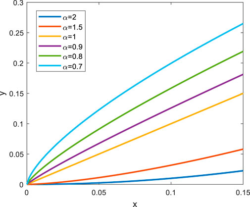
FIGURE 6. The curve of $y=x^{\mathrm{\alpha }}$ under different $\alpha$.

The evaluation term $r_1\left(t\right)$ of relative error, defined in formula 16, is used to evaluate the degree of deviation of the system state from the expected value. When the steady-state error is 0, $r_1\left(t\right)$ takes the maximum value of 0.

$r_1\left(t\right)={-\left|w_{1}re\left(t\right)\right|}^{{\alpha }_1}(16)$

where, ${\alpha }_1$ is the exponential adjustment factor, which can adjust the local feature. When ${\alpha }_1>1$, it means to reduce the local micro feature; when ${\alpha }_1<1$, it means to enlarge the local micro feature.

The evaluation item $r_2\left(t\right)$ of the reciprocal of the relative error, defined in formula 17, is used to evaluate the degree of fluctuation of the system state. When the system state is stable, $r_2\left(t\right)$ takes the maximum value of 0.

$r_2\left(t\right)={-\left|w_2\frac{\partial re\left(t\right)}{\partial t}\right|}^{{\alpha }_2}(17)$

where ${\alpha }_2$ is the exponential adjustment factor, its effect is consistent with that of ${\alpha }_1$.

In order to prevent the influence of parameter mutation in the control process, especially in the case of sudden step of reference value, the reciprocal of error is very large. Therefore, we built a $clip$ function, as shown in formula 18, which can limit the value to a certain range.

$clip\left(a,b,x\right)=\left\{\begin{array}{c}a,x>a\\ x,x\le a\\ b,x<b\end{array}\right.(18)$

The $clip$ function is used to process $r_2\left(t\right)$, and the following results are obtained:

$r_2^{\prime }\left(t\right)=clip\left(1,-1,r_2\left(t\right)\right)(19)$

By adding $r_1\left(t\right)$ and $r_2^{\prime }\left(t\right)$, the reward function of the low error area is obtained:

$r_3\left(t\right)=r_1\left(t\right)+r_2^{\prime }\left(t\right)(20)$

In summary, the final reward function is obtained:

$r\left(t\right)=\left\{\begin{array}{c}-100,\left|re\left(t\right)\right|>200\%\\ -2,15\%<\left|re\left(t\right)\right|\le 200\%\\ r_3\left(t\right),\left|re\left(t\right)\right|<15\%\end{array}\right.(21)$

In order to reduce the complexity, this paper defines ${\alpha }_1={\alpha }_2$ and to determine the values of ${\alpha }_1$ and ${\alpha }_2$, a water level tracking simulation experiment was carried out. The power level of the model used is 5%. At 10s, the water level reference value is adjusted from 0 mm to 100 mm, the simulation time is set to 600s, and the number of trainings is set to 1,200. At the end of the training, we tested the best performance of the agent obtained under different parameters as shown in Table 4, from which we can see that when ${\alpha }_1,{\alpha }_2=0.8$, the shortest setting time can be obtained, indicating that good control effect can be obtained at this time.

TABLE 4

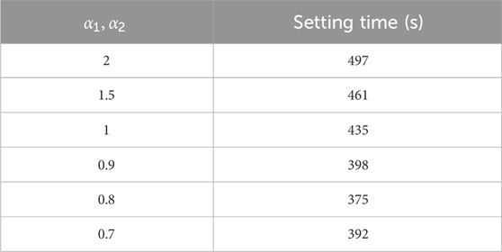
TABLE 4. Test results under different values of ${\alpha }_1$ and ${\alpha }_2$.

4 Results and discussion

4.1 Training results

In this paper, the water level adjustment performance is trained to obtain the best control performance. The detailed training content is consistent with Section 3.5. The main parameter Settings of the program are given in Table 5, which are determined by suggestions given in paper (Mnih et al., 2015) and several experimental tests.

TABLE 5

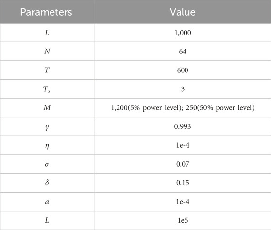
TABLE 5. Parameter settings.

Considering that similar results can be achieved across different power levels, we present training results for only the 5% power level and 50% power level. These training results are depicted in Figure 7. From the figures, it becomes evident that in the initial stages of the training process, when the agent has not yet collected sufficient experience and undergone an insufficient number of training steps, the episode reward remains low, indicating an exploratory phase. As the number of episodes increases, the agent progressively discerns patterns, and the control performance improves. During this phase, the episode reward exhibits an upward trend. After a substantial number of training episodes, the agent starts to converge, with convergence values around −220 for the 5% power level and around −315 for the 50% power level. During this period, there is no distinct trend in episode rewards, signifying that the optimal control policy has been achieved.

FIGURE 7

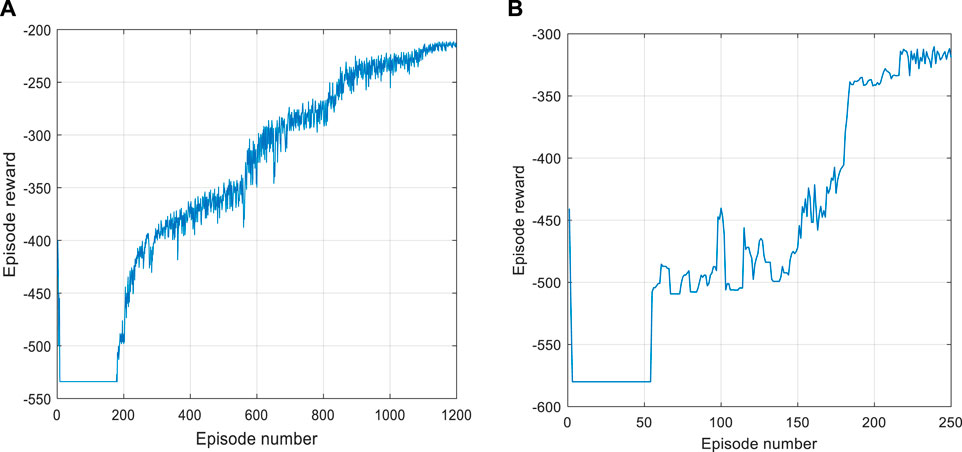
FIGURE 7. Training results. (A) Training results at 5% power level; (B) Training results at 50% power level.

Subsequently, an assessment of the trained controller’s performance is scheduled, encompassing three distinctive tests: a water level tracking test, an anti-interference test, and a comparative analysis against findings within publicly available literature. Concurrently, two meticulously optimized controllers, distinguished by their commendable performance, serve as benchmarking mechanisms for each power level. The first of these controllers, christened ‘FCPI,’ benefits from parameter optimization via a fuzzy logic algorithm, incorporating modules such as fuzzification, fuzzy rules, fuzzy inference, and defuzzification. The FCPI controller parameters can adapt with both power levels and water level errors. Due to space constraints, readers are encouraged to refer to the paper (Liu et al., 2010; Aulia et al., 2021) for details on the configuration strategy. The second controller, known as ‘ACPI,’ attains its optimized parameters through the gain scheduling algorithm and the relationship between the parameters of the CPI controller and power $p$ is expressed by formula 22.

$\left\{\begin{array}{l}kp1=-0.5991*p^3+0.6281*p^2+0.7725*p-0.0018\\ kp2=100-\frac{90}{1+{\left(\frac{p}{0.3117}\right)}^{-32.68}}\\ ki1=8.97*{10}^{-6}*\log 2\left(p\right)+4.876*{10}^{-5}\\ ki2=1\end{array}\right.(22)$

In order to gauge the efficacy of control, we use the evaluation indices ITSE and ITAE. These indices have been thoughtfully introduced, as they offer a practical framework for assessing the performance of the control system. They effectively encapsulate the system’s precision and responsiveness, with smaller values indicating superior performance.

$ITSE={\int }_0^{\infty }t{e}^2\left(t\right)dt(23)$

$ITAE={\int }_0^{\infty }t\left|e\left(t\right)\right|dt(24)$

where $e\left(t\right)$ is the error.

4.2 Test 1 water level tracking test

This section mainly tests the system’s output response under the action of step function, so as to show the dynamic performance of the system. The initial value of the reference water level is set to 0mm, and then jumps to 100 mm at 10s. The control effects of the three methods are compared at low power level (5%), medium power level (50%) and high power level (100%), respectively.

Figures 8, 9, 10 show the comparison results of the three methods at different power levels. It can be seen from these figures that the three methods can track the change of water level and have good control effect. At the low power level, the proposed method achieves a rise time of 73.9 s, which is 23.5% faster than the FCPI method and 59.4% faster than the ACPI method. At the medium power level, the proposed method achieves a rise time of 13.6 s, which is 29.6% faster than the FCPI method and 56.5% faster than the ACPI method. At the high power level, the proposed method achieves a rise time of 16.4 s, which is 10.4% faster than the FCPI method and 28.6% faster than the ACPI method. The above statements emphasize that the proposed method offers a faster response speed and superior control performance in terms of water level tracking. The proposed method, IHA, can iteratively engage with the steam generator model to acquire the water level control strategy. It employs deep neural networks to comprehend the intricate nonlinear relationship between system states and optimized actions. This adaptation allows the controller parameters to accommodate the dynamic variations of the system without the necessity of manual design for optimization strategies, as required in methods like FCPI and ACPI. Given the prolonged delay in false water level generation and the extended response time in low-power scenarios, more time is required to achieve control.

FIGURE 8

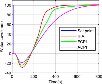
FIGURE 8. Water level tracking test results at 5% power level.

FIGURE 9

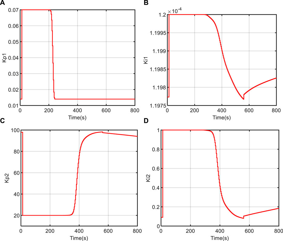
FIGURE 9. The test results of water level tracking at 50% power level. (A) Kp1; (B) Ki1; (C) Kp2; (D) Ki2.

FIGURE 10

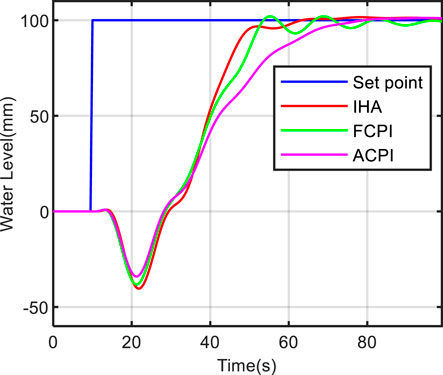
FIGURE 10. The test results of water level tracking at 100% power level.

Table 6 shows the comparison results of ITSE and ITAE of different methods, from which under different power levels, the values of ITSE and ITAE are IHA < FCPI < ACPI. At the low power level, the proposed method exhibits an ITSE that is 10.7% lower than FCPI and 38.4% lower than ACPI. Additionally, the ITAE of the proposed method is 26.2% lower than FCPI and 83.3% lower than ACPI. At the medium power level, the proposed method achieves an ITSE that is 1.3% lower than FCPI and 7.1% lower than ACPI. Furthermore, the ITAE of the proposed method is 6.2% lower than FCPI and 23.7% lower than ACPI. At the high power level, the proposed method demonstrates an ITSE that is 3.2% lower than FCPI and 10.3% lower than ACPI. Likewise, the ITAE of the proposed method is 6.8% lower than FCPI and 20.7% lower than ACPI. The statements above highlight that the IHA method excels in terms of control accuracy and speed, particularly evident at low power levels. In summary, the IHA method exhibits the best control performance, followed by FCPI and ACPI, which aligns with the conclusions drawn from the figures.

TABLE 6

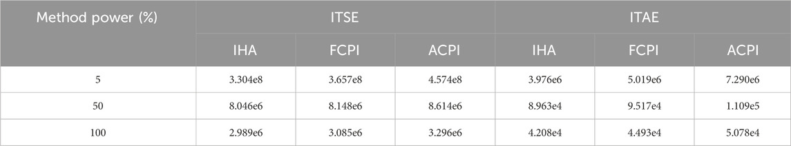
TABLE 6. The ITSE and ITAE of different method.

Figures 11, 12, 13 depict the variation curves of the IHA controller parameters $Kp1$, $Ki1$, $Kp2$, and $Ki2$ at different power levels. It is evident that the controller parameters adaptively change with the system’s state during the control process. In theory, the integral coefficient $Ki$ of the PI controller primarily works to reduce steady-state error, while the proportional coefficient Kp reflects the system’s response speed, rapidly reducing error. Consequently, $Ki$ has a noticeable effect towards the end of the control process, whereas $K{p}^{\prime }s$ impact is more pronounced in the early stages. In the parameter curve results, when the water level error is significant, the proportional coefficient $Kp1$ plays a major role. At such times, $Kp1$ assumes larger values across all three power levels, such as the time range for the 5% power level from 10s to 200s, the 50% power level from 10s to 37s, and the 100% power level from 10s to 25s. However, the integral coefficient shows no distinct pattern because it has little influence when the error is substantial. As the water level error decreases, the value of $Kp1$ decreases as well, reducing the likelihood of overshoot. For instance, the time range for the 5% power level shifts to 200s–350s, the 50% power level to 37s–50s, and the 100% power level to 25s–40s. When the error approaches zero, $Kp1$ stabilizes and does not have a fixed value, while $Ki1$ and $Ki2$ generally assume larger values. This is because when the error is zero, $Kp1$ has minimal effect, and increasing the integral coefficient is beneficial for reducing steady-state error. Simultaneously, $Kp2$ does not exhibit a clear pattern throughout the control cycle. Furthermore, manual parameter adjustments reveal that $Kp2$ has little influence on the results within a certain range. Hence, under varying power levels, the proposed method can autonomously generate optimized strategies for the CPI controller parameters ($Kp1$, $Kp2$, $Ki1$, $Ki2$) based on the system’s state. This assurance ensures that the system can efficiently regulate the water level to the specified position in the shortest possible time, optimizing overall performance.

FIGURE 11

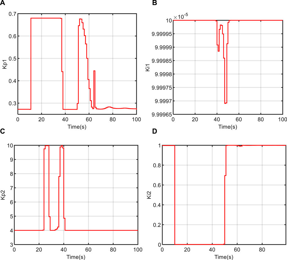
FIGURE 11. The changing curve of controller parameters at 5% power level. (A) Kp1; (B) Ki1; (C) Kp2; (D) Ki2.

FIGURE 12

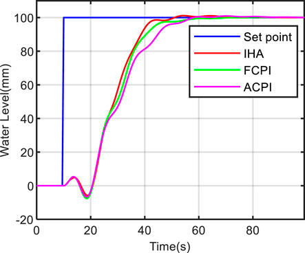
FIGURE 12. The changing curve of controller parameters at 50% power level.

FIGURE 13

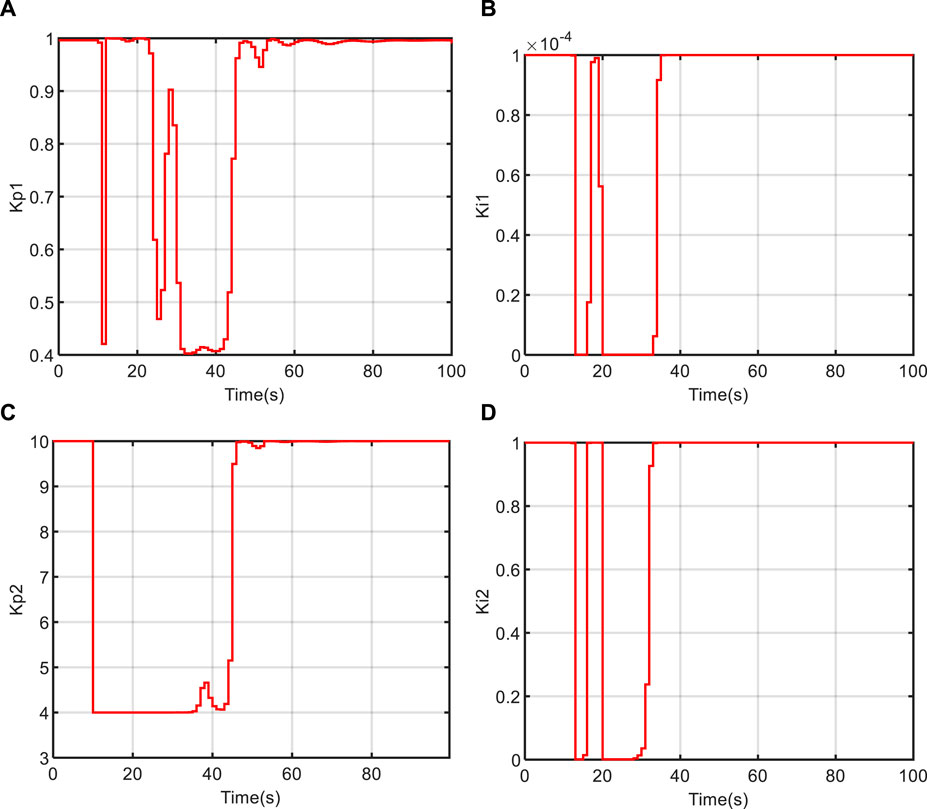
FIGURE 13. The changing curve of controller parameters at 100% power level. (A) Kp1; (B) Ki1; (C) Kp2; (D) Ki2.

Under the work of the ACPI method, the control law can adapt to changes in power levels but struggles to adapt effectively to variations in water level states. Consequently, the ACPI method falls short of achieving an optimal control effect. The FCPI method, while capable of adjusting the control law adaptively with both power level and water level state, relies heavily on the design of fuzzy membership functions and fuzzy rules, which are inherently influenced by human experience. This design challenge makes it difficult to encompass all possible system states, making it also challenging for the FCPI method to achieve an optimal control effect. However, the proposed method excels in achieving an ideal control effect across all power levels, primarily due to its efficient reinforcement learning mechanism. Throughout the control process, both gain and control law can adaptively evolve in response to changes in power levels and state information. During the learning process, the controller agent accumulates control experience continuously through repeated interactions with the environment. It autonomously learns from this experience and explores new strategies within the control policy space. Over time, the controller agent matures and evolves into a master of control, thus achieving exceptional control performance.

4.3 Test 2 anti-interference test

To assess the anti-interference capability of the proposed controller, we conducted a steam flow disturbance benchmark test on models at different power levels. During the test, a step disturbance in steam flow of +35.88 kg/s was introduced at 10 s (Liu et al., 2010; Ansarifar et al., 2012). The test results are depicted in Figures 14, 15, 16. From these figures, it is evident that all three methods exhibit strong anti-interference capabilities and swiftly restore the water level to its normal state. Moreover, the oscillation amplitude and adjustment time of the water level decrease as the power level increases, signifying more efficient water level control at higher power levels compared to lower ones. Notably, at the 5% power level, the proposed method restores the water level to its normal state in approximately 200 s in Figure 14A, outperforming the FCPI and ACPI methods. This rapid recovery demonstrates the exceptional anti-interference performance of the IHA controller across various power levels. In Figure 14B- Figure 16B, we observe the changes in feed water flow and steam flow under the control of the IHA method. It is apparent that the feed water flow quickly tracks the variations in steam flow. However, due to the non-minimum phase characteristics of the system at low power levels, the system’s recovery time is longer in this scenario.

FIGURE 14

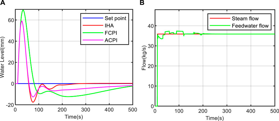
FIGURE 14. Anti-interference test result at 5% power level. (A) water level change curve; (B) flow change curve.

FIGURE 15

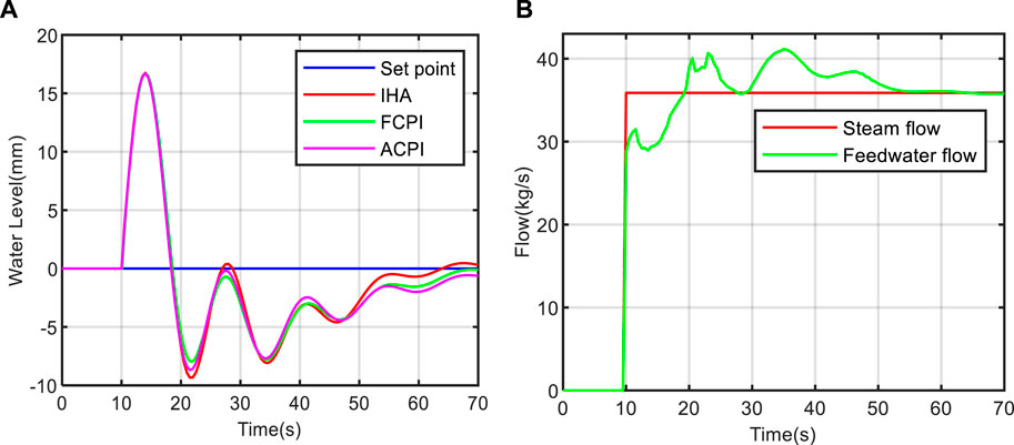
FIGURE 15. Anti-interference test result at 50% power level. (A) water level change curve; (B) flow change curve.

FIGURE 16

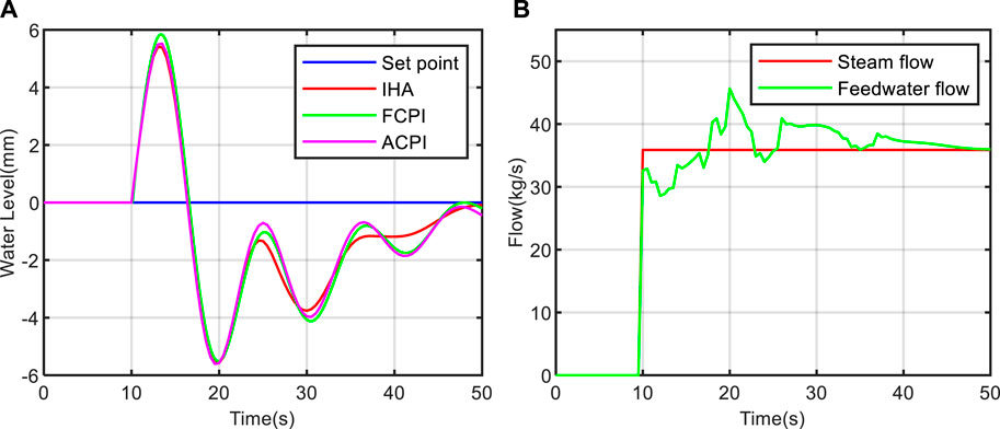
FIGURE 16. Anti-interference test result at 100% power level. (A) water level change curve; (B) flow change curve.

Table 7 provides a comparison of ITSE and ITAE results in the anti-interference tests of different methods. At the 5% power level, the ITSE of the IHA method is 77.8% lower than that of FCPI and 34.2% lower than that of ACPI. Similarly, the ITAE of the IHA method is 84.4% lower than that of FCPI and 70.2% lower than that of ACPI. These results clearly demonstrate that the IHA method outperforms the other two methods significantly in terms of both ITSE and ITAE at the 5% power level. Conversely, the comparison results among the three methods show similarity at the 50% and 100% power levels, which aligns with the observations in Figure 14A- Figure 16A.

TABLE 7

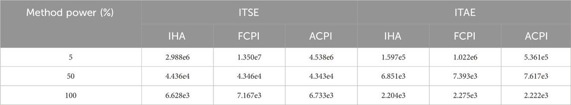
TABLE 7. The comparison results of ITSE and ITAE of different methods.

In summary, the proposed method exhibits a strong anti-interference effect, particularly evident at certain power levels. However, it does not consistently demonstrate clear advantages across all power levels. This limitation stems from the focus of this paper, which primarily investigated water level tracking tasks during the training process of deep reinforcement learning. The development of a comprehensive anti-interference strategy is a potential area for future optimization and research.

4.4 Test 3 comparison of research results with public literature

It is well known that the water level of UTSG is the most difficult to control at low power level (Choi et al., 1989). In order to highlight the advantages of the proposed method at low power level, we compare the water level tracking effect of the IHA controller at 5% power level with the research results in the public literature, and the test content is to adjust the water level from 0mm to 100 mm.

The setting time serves as the evaluation index, defined as the minimum time required for the water level to reach and stabilize within ±5% of the set value. The comparison results are shown in Table 8, from which we can see that the proposed method can shorten the adjustment time to 375s, with a considerable advantage over other methods, fully embodies the advantages of reinforcement learning.

TABLE 8

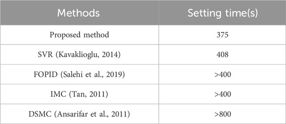
TABLE 8. Comparison results.

To underscore the merits of the proposed method under conditions of low power level, we juxtapose the water level tracking efficacy of the IHA controller at a power level of 5% with the discoveries derived from other public research. The experimental setting entails the modulation of water levels ranging from 0mm to 100 mm. It is worth noting that the referenced investigations introduced methodologies such as SVR, FOPID, IMC, and DSMC, all of which featured test content and equipment models consistent with our current study. Consequently, this paper directly assimilates their resultant data for the purpose of comparative scrutiny.

5 Conclusion

Aiming at the water level control of UTSG, an intelligent controller IHA based on CPI controller and DRL is proposed in this paper, which does not require prior knowledge of the model’s dynamic characteristics. Instead, it autonomously explores the model during the training process, gathers pertinent data, and subsequently leverages this experience to iteratively enhance control performance. Through extensive training, this approach yields a controller with commendable control performance and robustness. The primary contributions of this paper are outlined as follows:

(1) A new reward function is proposed to evaluate the control effect and improve the training quality. The results demonstrate significant improvements in training effectiveness, offering valuable insights for other analogous control systems.

(2) The application of the DDPG algorithm for learning the CPI control policy, enabling the algorithm to accumulate experience through continuous exploration of the environment, without heavy reliance on extensive expert experience. After continuous training, the model’s performance stabilizes and ultimately converges to an ideal state, with convergence values reaching approximately −220 for the 5% power level and about −315 for the 50% power level.

(3) In the water level tracking test, at low, medium, and high power levels, the proposed method achieves rise times of 73.9 s, 13.6 s, and 16.4 s, respectively. These results indicate superior control performance compared to other methods, and the controller parameters can be dynamically adjusted based on the system’s state. When contrasted with outcomes from traditional control algorithms and publicly available literature, the substantial reduction in setting time clearly demonstrates the evident advantages of the proposed method.

(4) In the anti-interference test, at low power levels, the IHA controller can restore the water level to its normal state within 200 s, which is considerably faster than other methods. Additionally, the feed water flow promptly adapts to variations in steam flow, effectively mitigating the impact of steam flow disturbances on the water level.

In summary, the controller proposed in this paper demonstrates effective control across various power levels, as reinforcement learning autonomously learns optimization strategies for controller parameters without relying on expert knowledge. However, it is crucial to acknowledge that the designed control method has been exclusively validated on the steam generator model presented in this paper, yielding favorable results. Its efficacy has not been verified for water level control in other steam generator models, presenting a challenge for our team to address in the future. Given the operational similarities among different steam generator models, our team aims to transfer the acquired control strategies to other models through imitation learning, thereby achieving the migration of advanced control strategies.

Data availability statement

The original contributions presented in the study are included in the article/Supplementary Material, further inquiries can be directed to the corresponding author.

Author contributions

BP: Methodology, Software, Validation, Writing–original draft, Writing–review and editing. XM: Supervision, Validation, Writing–review and editing. HX: Funding acquisition, Resources, Validation, Writing–review and editing.

Funding

The author(s) declare financial support was received for the research, authorship, and/or publication of this article. This project was supported by the China North Artificial Intelligence & Innovation Research Institute and the Natural Science Foundation of Heilongjiang Province, China (Grant NO. E2017023).

Conflict of interest

Author XM was employed by China Nuclear Power Engineering Co, Ltd.

The remaining authors declare that the research was conducted in the absence of any commercial or financial relationships that could be construed as a potential conflict of interest.

Publisher’s note

All claims expressed in this article are solely those of the authors and do not necessarily represent those of their affiliated organizations, or those of the publisher, the editors and the reviewers. Any product that may be evaluated in this article, or claim that may be made by its manufacturer, is not guaranteed or endorsed by the publisher.

Abbreviations

ACPI, Adaptive Cascaded Proportional-Integral; CPI, Cascaded Proportional-Integral; DDPG, Deep Deterministic Policy Gradients; DRL, Deep reinforcement learning; FCPI, Fuzzy Cascaded Proportional-Integral; IHA, Intelligent hierarchical autonomous; ITAE, Integral of time weighted absolute error; ITSE, integral of time weighted squared errors; PID, Proportional-Integral-Derivative; PWR, Pressurized Water Reactors; ResNet, Residual neural network; RL, Reinforcement learning; UTSG, U-Tube Steam Generator.

References

Ahmmed, T., Akhter, I., Rezaul Karim, S. M., and Sabbir Ahamed, F. A. (2020). Genetic algorithm based PID parameter optimization. Am. J. Intelligent Syst. 10 (1), 8–13. doi:10.5923/j.ajis.20201001.02

CrossRef Full Text | Google Scholar

Ansarifar, G. R., Davilu, H., and Talebi, H. A. (2011). Gain scheduled dynamic sliding mode control for nuclear steam generators. Prog. Nucl. Energy 53, 651–663. doi:10.1016/j.pnucene.2011.04.029

CrossRef Full Text | Google Scholar

Ansarifar, G. R., Talebi, H. A., and Davilu, H. (2012). Adaptive estimator-based dynamic sliding mode control for the water level of nuclear steam generators. Prog. Nucl. Energy 56, 61–70. doi:10.1016/j.pnucene.2011.12.008

CrossRef Full Text | Google Scholar

Aulia, D. P., Yustin, A. S., Hilman, A. M., Annisa, A. R., and Wibowo, E. W. K. (2021). “Fuzzy gain scheduling for cascaded PI-control for DC motor,” in 5th IEEE Conference on Energy Conversion, CENCON 2021, Johor Bahru, Malaysia, 25-25 October 2021. doi:10.1109/CENCON51869.2021.9627292

CrossRef Full Text | Google Scholar

Bi, C., Pan, G., Yang, L., Lin, C. C., Hou, M., and Huang, Y. (2019). Evacuation route recommendation using auto-encoder and Markov decision process. Appl. Soft Comput. J. 84, 105741. doi:10.1016/j.asoc.2019.105741

CrossRef Full Text | Google Scholar

Carapuço, J., Neves, R., and Horta, N. (2018). Reinforcement learning applied to Forex trading. Appl. Soft Comput. J. 73, 783–794. doi:10.1016/j.asoc.2018.09.017

CrossRef Full Text | Google Scholar

Choi, J. I., Meyer, J. E., and Lanning, D. D. (1989). Automatic controller for steam generator water level during low power operation. Nucl. Eng. Des. 117, 263–274. doi:10.1016/0029-5493(89)90175-1

CrossRef Full Text | Google Scholar

He, K., Zhang, X., Ren, S., and Sun, J. (2016). “Deep residual learning for image recognition,” in Proceedings of the IEEE Computer Society Conference on Computer Vision and Pattern Recognition, Las Vegas, NV, USA, 27-30 June 2016, 770–778. doi:10.1109/CVPR.2016.90

CrossRef Full Text | Google Scholar

Hu, X., and Liu, J. (2020). “Research on UAV balance control based on expert-fuzzy adaptive PID,” in Proceedings of 2020 IEEE International Conference on Advances in Electrical Engineering and Computer Applications, AEECA 2020, Dalian, China, 25-27 August 2020. doi:10.1109/AEECA49918.2020.9213511

CrossRef Full Text | Google Scholar

Irving, E., Miossec, C., and Tassart, J. (1980). Towards efficient full automatic operation of the pwr steam generator with water level adaptive control, 309–329.

Google Scholar

Jia, Y., Chai, T., Wang, H., and Su, C. Y. (2020). A signal compensation based cascaded PI control for an industrial heat exchange system. Control Eng. Pract. 98, 104372. doi:10.1016/j.conengprac.2020.104372

CrossRef Full Text | Google Scholar

Kavaklioglu, K. (2014). Support vector regression model based predictive control of water level of U-tube steam generators. Nucl. Eng. Des. 278, 651–660. doi:10.1016/j.nucengdes.2014.08.018

CrossRef Full Text | Google Scholar

Kong, X., Shi, C., Liu, H., Geng, P., Liu, J., and Fan, Y. (2022). Performance optimization of a steam generator level control system via a revised simplex search-based data-driven optimization methodology. Processes 10, 264. doi:10.3390/pr10020264

CrossRef Full Text | Google Scholar

Li, C., Mao, Y., Zhou, J., Zhang, N., and An, X. (2017). Design of a fuzzy-PID controller for a nonlinear hydraulic turbine governing system by using a novel gravitational search algorithm based on Cauchy mutation and mass weighting. Appl. Soft Comput. J. 52, 290–305. doi:10.1016/j.asoc.2016.10.035

CrossRef Full Text | Google Scholar

Lillicrap, T. P., Hunt, J. J., Pritzel, A., Heess, N., Erez, T., Tassa, Y., et al. (2016). “Continuous control with deep reinforcement learning,” in 4th International Conference on Learning Representations, ICLR 2016 - Conference Track Proceedings.

Google Scholar

Liu, C., Zhao, F. Y., Hu, P., Hou, S., and Li, C. (2010). P controller with partial feed forward compensation and decoupling control for the steam generator water level. Nucl. Eng. Des. 240, 181–190. doi:10.1016/j.nucengdes.2009.09.014

CrossRef Full Text | Google Scholar

Maghfiroh, H., Ahmad, M., Ramelan, A., and Adriyanto, F. (2022). Fuzzy-PID in BLDC motor speed control using MATLAB/simulink. J. Robotics Control (JRC) 3, 8–13. doi:10.18196/jrc.v3i1.10964

CrossRef Full Text | Google Scholar

Mnih, V., Kavukcuoglu, K., Silver, D., Rusu, A. A., Veness, J., Bellemare, M. G., et al. (2015). Human-level control through deep reinforcement learning. Nature 518, 529–533. doi:10.1038/nature14236

PubMed Abstract | CrossRef Full Text | Google Scholar

Rao, Y., Hao, J., and Chen, W. (2024). Calculate of an additional resistance with reverse flow in steam generator under steady-state conditions. Ann. Nucl. Energy 198, 110302. doi:10.1016/J.ANUCENE.2023.110302

CrossRef Full Text | Google Scholar

Rodriguez-Abreo, O., Rodriguez-Resendiz, J., Fuentes-Silva, C., Hernandez-Alvarado, R., and Falcon, M. D. C. P. T. (2021). Self-tuning neural network PID with dynamic response control. IEEE Access 9, 65206–65215. doi:10.1109/ACCESS.2021.3075452

CrossRef Full Text | Google Scholar

Safarzadeh, O., Khaki-Sedigh, A., and Shirani, A. S. (2011). Identification and robust water level control of horizontal steam generators using quantitative feedback theory. Energy Convers. Manag. 52, 3103–3111. doi:10.1016/j.enconman.2011.04.023

CrossRef Full Text | Google Scholar

Salehi, A., Safarzadeh, O., and Kazemi, M. H. (2019). Fractional order PID control of steam generator water level for nuclear steam supply systems. Nucl. Eng. Des. 342, 45–59. doi:10.1016/j.nucengdes.2018.11.040

CrossRef Full Text | Google Scholar

Sen Peng, B., Xia, H., Liu, Y. K., Yang, B., Guo, D., and Zhu, S. M. (2018). Research on intelligent fault diagnosis method for nuclear power plant based on correlation analysis and deep belief network. Prog. Nucl. Energy. 108, 419–427. doi:10.1016/j.pnucene.2018.06.003

CrossRef Full Text | Google Scholar

Sui, Z. G., Yang, J., Zhang, X. Y., and Yao, Y. (2020). Numerical investigation of the thermal-hydraulic characteristics of AP1000 steam generator U-tubes. Int. J. Adv. Nucl. React. Des. Technol. 2, 52–59. doi:10.1016/j.jandt.2020.09.001

CrossRef Full Text | Google Scholar

Sutton, R. S., McAllester, D., Singh, S., and Mansour, Y. (2000). Policy gradient methods for reinforcement learning with function approximation. Adv. Neural Inf. Process. Syst., 1057–1063.

Google Scholar

Tan, W. (2011). Water level control for a nuclear steam generator. Nucl. Eng. Des. 241, 1873–1880. doi:10.1016/j.nucengdes.2010.12.010

CrossRef Full Text | Google Scholar

Thomas, P. S., and Brunskill, E. (2017). Policy gradient methods for reinforcement learning with function approximation and action-dependent baselines. arXiv preprint arXiv:1706.06643. Available at: https://doi.org/10.48550/arXiv.1706.06643.

Google Scholar

Uhlenbeck, G. E., and Ornstein, L. S. (1930). On the theory of the Brownian motion. Phys. Rev. 36, 823–841. doi:10.1103/PhysRev.36.823

CrossRef Full Text | Google Scholar

Wan, J., He, J., Li, S., and Zhao, F. (2017). Dynamic modeling of AP1000 steam generator for control system design and simulation. Ann. Nucl. Energy 109, 648–657. doi:10.1016/j.anucene.2017.05.016

CrossRef Full Text | Google Scholar

Wang, Z., and Hong, T. (2020). Reinforcement learning for building controls: the opportunities and challenges. Appl. Energy 269, 115036. doi:10.1016/j.apenergy.2020.115036

CrossRef Full Text | Google Scholar

Xu, X., and Li, D. (2020). Torque control of DC torque motor based on expert PID. J. Phys. Conf. Ser. 1626, 012073. doi:10.1088/1742-6596/1626/1/012073

CrossRef Full Text | Google Scholar

Zhang, L., Li, S., Xue, Y., Zhou, H., and Ren, Z. (2022). Neural network PID control for combustion instability. Combust. Theory Model. 26, 383–398. doi:10.1080/13647830.2022.2025908

CrossRef Full Text | Google Scholar

Zhou, M., Wang, Y., and Wu, H. (2019). Control design of the wave compensation system based on the genetic PID algorithm. Adv. Mater. Sci. Eng. 2019, 1–13. doi:10.1155/2019/2152914

CrossRef Full Text | Google Scholar

Zhu, Z., Liu, Y., He, Y., Wu, W., Wang, H., Huang, C., et al. (2022). Fuzzy PID control of the three-degree-of-freedom parallel mechanism based on genetic algorithm. Appl. Sci. Switz. 12 (21), 11128. doi:10.3390/app122111128

CrossRef Full Text | Google Scholar