Development of a fully implicit ODE-solver for containment analysis code

The thermal–hydraulic dynamics in containment are governed by a system of stiff ordinary differential equations (ODEs). A fully implicit discretization scheme is adopted to discretize these ODEs in order to mitigate the effects of stiffness. In comparison with explicit or semi-implicit discretization schemes that are subject to Courant limits on time steps, the fully implicit discretization scheme is more suitable for a containment analysis code that focuses on predicting both short-term and long-term thermal–hydraulic parameters after an accident. This study introduces a general-purpose ODE solver for the containment analysis code. The outline of the solver is as follows: The fully implicit discrete equations lead to a large set of nonlinear equations that need to be solved using Newton’s iterative method. The partial derivative components in the Jacobi matrix are calculated by the perturbation method using finite difference approximation, which avoids the complicated derivation of partial derivatives. The scaling modification technique is incorporated into this ODE solver to deal with significant differences in unknown variable magnitudes, and the line search method is introduced to address the difficulty of obtaining an accurate root estimate with Newton’s method when the initial guess is far from the actual root. This proposed ODE solver was applied to two typical stiff ODE problems to test its stiffness-suppressed ability and to demonstrate that this proposed solver can perform calculations with a very large time step. Then, the CASSIA code, a containment analysis code developed by China Nuclear Power Technology Research Institute Co., Ltd (CNPRI), equipped with this ODE solver, was applied to the CSNI (Committee on the Safety of Nuclear Installations) benchmark problem and the Carolinas Virginia Tube Reactor (CVTR) test 3 problem to preliminarily demonstrate that the proposed ODE solver can perform containment thermal–hydraulic analysis correctly. This study could provide references for the development of a home-made containment analysis code.

1 Introduction

The widespread utilization of nuclear energy has placed a heightened emphasis on nuclear safety, particularly following the Fukushima nuclear power plant accident in Japan (Chen et al., 2018). The containment structure serves as the ultimate safeguard against the release of radioactive fission products into the surrounding environment. Maintaining the structural integrity of the containment system during loss of coolant accidents (LOCA) or main steam line breaks (MSLB) necessitates the control of pressure and temperature within the structure to ensure that they remain below acceptable limits (Brosche D, 1972). It is crucial to gain a precise understanding of the time- and space-dependent pressure and temperature distribution within a containment to ensure reactor safety. Thus, the development of a reliable mathematical model and corresponding containment thermal–hydraulic code is crucial for accurate prediction of the time- and space-dependent pressure distribution within the containment structure.

The mathematical simulation of thermal–hydraulic dynamics within containment structures involves stiff initial value problems (IVPs) in ordinary differential equations (ODEs), which is shown as follows:

$\left\{\begin{array}{l}\frac{d\overrightarrow{y}}{dt}=\overrightarrow{F}\left(t,\overrightarrow{y}\right)\\ \overrightarrow{y}\left(t_0\right)={\overrightarrow{y}}_0.\end{array}\right.(1)$

Efficient and accurate numerical methods are essential for solving these types of problems. Conventional ODE solving methods, such as Euler (Butcher. (2008)), explicit Runge–Kutta (Butcher. (2008)), and Adams (Wille, (1998)), are restricted to a very small step size in order to achieve a stable solution. This means that substantial computer time could be required. To address this challenge, an implicit scheme, which is unconditionally stable, is required to allow for larger time steps and maintain stability regardless of the stiffness of the problem.

Consequently, either the semi-implicit method (the convection term is linerarized) or the fully implicit method is adopted by the traditional containment thermal–hydraulic analysis code. Vapor, liquid pool, and droplets are simulated in the CONTAIN 2.0 code (Murata et al., 1997). An implicit numerical method was used to calculate flow rates based on pressure and temperature in control volumes, and fluid inertia was neglected in the momentum equation. Complicated 1-D and 3-D conservation equations were considered in the advanced integral containment code, GOTHIC code (George et al., 2001). The semi-implicit method is adopted to solve momentum equations, and then mass and energy conservation equations are discretized by the semi-implicit method and solved by the one-step Newton–Raphson method. The conservation equations in the COCOSYS code (Allelein et al., 2008; O Dell and Wong, 2010) are discretized by the explicit or implicit method, and the Richardson extrapolation method is used to enhance the accuracy of results and improve convergence. Some severe accident analysis codes, like MELCOR (Gauntt et al., 2005), can also be used to analyze containment thermal hydraulic behaviors. Conservation equations in MELCOR were discretized by the semi-implicit method and solved by the fixed-point iteration method.

The velocity in the convection term of the momentum equation is linearized in the CONTAIN code, GOTHIC code, and MELCOR code, which means the time step used in these codes is restricted to the Courant limit, and its value should not exceed a certain value (Cai, 2022). The time step used in the COCOSYS code can reach a large value due to an optional numerical scheme adopted in this code, i.e., the fully implicit method, but the Richardson extrapolation method used to enhance the accuracy of results and improve convergence requires the calculation of additional solutions at different grid resolutions to estimate the error and refine the final solution. This process increases the computational cost of the simulation as it involves running the simulation multiple times with different grid sizes (Florez et al., 2017; Merga and Chemeda, 2021).

The system of differential equations for thermal–hydraulic dynamics is discretized via fully implicit schemes, yielding a set of nonlinear equations. Common methods for solving nonlinear equation systems include Newton’s iteration method (Press et al., 2007), the fixed-point iteration method (Hoffman and Frankel, 2001), and the trust-region method (Yuan, 2000). Considering the rapid convergence and effectiveness of Newton’s iteration method, this study adopts it for solving the nonlinear equation system resulting from fully implicit discretization. Consequently, in the present work, a Newton-based fully implicit ODE solver with a convergence-enhanced method is proposed for the containment analysis code CASSIA, which has been developed by China Nuclear Power Technology Research Institute Co., Ltd. (CNPRI).

Section 2 introduces the governing equations of the CASSIA code, necessary closure models, a discretization scheme, and a Newton-based solution procedure. Section 3 shows the application of this proposed ODE solver to two typical stiff ODE problems to test its stiffness-suppressed ability and to demonstrate that this proposed solver can perform calculations with a very large time step. Then, Section 4 shows the application of the CASSIA code equipped with this ODE solver to the CNSI benchmark problem and the Carolinas Virginia Tube Reactor (CVTR) test 3 problem to preliminarily demonstrate that the proposed ODE solver can perform containment thermal–hydraulic analysis correctly.

2 Overview of a fully implicit ODE solver for containment code

2.1 Governing equations for containment analysis code

2.1.1 Basic conservation equations

The basic computational components in the containment analysis code are control volume, junction, and heat structure. They are used to model the compartments, connections between compartments, and compartment walls in containment, respectively. These computational components are illustrated in Figure 1; the left component represents a control volume with a pool, while the right component represents a control volume without a pool. The junction connects these two control volumes. On the right side of the right control volume, there is a heat structure component used to represent heat transfer between this control volume and another control volume or with the environment. The sump water and gas mixture in a control volume is based on the thermal non-equilibrium assumption, which allows them to have different temperatures. The droplet within the containment compartment is conveyed through the gas junction, taking into account the thermal–hydraulic state (saturated or superheated) of the target volume. If the target volume becomes superheated, the droplet undergoes evaporation.

Figure 1

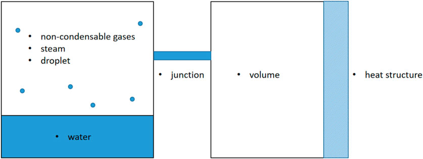
Figure 1. Illustration of volume, junction, and heat structure in the containment code.

The basic governing equations for containment thermal–hydraulic calculations are shown as follows (if droplets exist, the governing equations for droplets are also needed):

The mass conservation equations are as follows:

$\frac{d{M}_{steam}}{dt}=G_{steam,}(2)$

$\frac{d{M}_i}{dt}=G_i\left(i=1,\cdots ,m\right),(3)$

$\frac{d{M}_{water}}{dt}=G_{water}.(4)$

Eqs (2)–(4) delineate the mass conservation of the steam component (denoted by the subscript “steam”) and all m types of non-condensable gas components (denoted by the subscript “i") within the upper gas phase sub-volume. The subscript “water” signifies the water component within the lower liquid phase sub-volume. Furthermore, M represents mass, while G denotes the mass flow rate.

The energy conservation equations are as follows:

$\begin{array}{l}\frac{d}{dt}\left({\displaystyle \sum _{i=1}^m}{M}_i{h}_i+M_{steam}{h}_{steam}\right)-V_{gas}\\ \frac{dp}{dt}={\displaystyle \sum _k}\left({\displaystyle \sum _{j=1}^{N_{in}}}{G}_{k,j}{h}_{i,j}-{\displaystyle \sum _{j=1}^{N_{out}}}{G}_{k,j}{h}_{k,j}\right)+{\dot{Q}}_{gas,in}-{\dot{Q}}_{gas,out},\end{array}(5)$

$\begin{array}{l}\frac{d}{dt}\left(M_{water}{h}_{water}\right)-V_{water}\frac{dp}{dt}\\ =\sum \left(G_{water,in}{h}_{water,in}-G_{water,out}{h}_{water,out}\right)\\ +{\dot{Q}}_{water,in}-{\dot{Q}}_{water,out.}\end{array}(6)$

Eqs (5) and (6) describe the conservation of energy within the gas phase sub-volume (denoted by the subscript “gas”) and the liquid phase sub-volume (denoted by the subscript “water”). In Eq (5), the first term on the left-hand side represents the change rate of total energy in the gas phase sub-volume, while the second term represents the work performed by volume expansion. On the right-hand side of the equation, the first term accounts for the energy exchange due to the flow of all gas components, where the subscript “in” denotes inflow to the control volume and “out” denotes outflow from the control volume. The summation variable “k” encompasses all gas components, while “N_in” and “N_out” represent the number of fluids flowing into and out of the control volume, respectively. The term “$\dot{Q}$” denotes energy exchange, such as evaporation and condensation at the gas–liquid interface, and energy transfer into and out of the control volume via heat structures. Eq. (6) is similar to Eq. (5), and its details are omitted here for brevity. In addition, h is the specific enthalpy.

There are two different kinds of junctions (gas junctions and water junctions), considering the characteristics of flow inside the containment. Taking a gas junction as an example, the mass flow rate is calculated by the following equations:

$\frac{d\overrightarrow{G}}{dt}=\frac{A}{l}\left[\rho g\left(e{l}_{out}-e{l}_{in}\right)+\left(p_{out}-p_{in}\right)-\xi \frac{1}{2\rho A^2}\overrightarrow{G}\left|\overrightarrow{G}\right|\right],(7)$

$\rho =\frac{1}{2}\left({\rho }_{out}+{\rho }_{in}\right),(8)$

$\xi ={\xi }_0+{\xi }_a,(9)$

where A represents the cross-sectional area of the junction, l is the length of the junction, and ρ is the density of the fluid inside the junction, which is calculated as the arithmetic mean of the gas mixture density inside the control volume at the two ends of the junction (as shown in Eq. 8). el_out and el_in are the elevations of the outlet and inlet of the junctions, respectively; p_out and p_in are the pressures at the outlet and inlet of the junction, respectively; and ζ is the resistance coefficient of the junction, which is composed of the user-input local resistance coefficient and the frictional resistance coefficient along the junction (calculated by empirical formulas).

The volume conservation equation is as follows:

$V_{gas}+V_{water}=const.(10)$

Eq. 10 indicates that the total volume of the control volume remains constant.

Physically, the entire equation system of differential equations from Eqs (2–7) exhibits rapid pressure responses with slower temperature and energy responses, leading to a significant disparity in the time scales of the dynamics, which qualitatively characterizes the system as a stiff equation set. Mathematically, if the condition number of the Jacobian matrix of the discretization equation for the ODEs is excessively large, the equation system can be considered stiff [(Butcher. (2008)); Thohura and Rahman, (2013).]. As an example, the condition number of the Jacobian matrix (the matrix is shown in Table 1) for the initial time step of the CNSI benchmark problem, which is simulated in Section 4.1, is calculated (the condition number is equal to $4.5737\cdot {10}^{13}$), indicating that the problems to be solved by the containment code constitute a stiff equation set as well.

Table 1

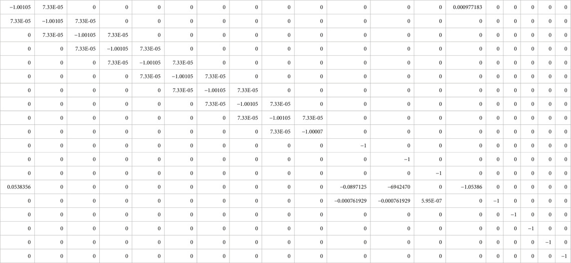
Table 1. Jacobian matrix for the CNSI benchmark problem.

To mitigate the effects of stiffness, a fully implicit discretization scheme is employed for solving the ordinary differential equations (ODEs) involved in the containment analysis code. In contrast to the explicit or semi-implicit discretization schemes, which are subject to Courant limits on time steps, the fully implicit discretization scheme is better suited for predicting both short-term and long-term thermal–hydraulic parameters following an accident.

2.1.2 Wall heat transfer equations

The heat transfer between containment walls and the gas mixture in the containment is taken into account by heat conduction through the wall, which is modeled by a heat structure as shown in Figure 1. The one-dimensional heat conduction model is adopted here. Although the three-dimensional heat conduction model considering the axial and circumferential temperature variations of the containment walls and internal heat sink is more accurate, only the heat conduction in the direction perpendicular to the containment wall (i.e., the radial direction) is considered here due to the axial temperature and circumferential gradients being minimal compared with radial gradients. The code uses the finite difference method to solve the heat conduction problem.

The one-dimensional heat conduction equation (as mentioned above, the radial direction is the direction of heat conduction) is presented as follows:

$\rho C_p\frac{\partial T}{\partial t}=k\frac{{\partial }^{2}T}{\partial x^2},(11)$

where k is the thermal conductivity, t is the time, T is the temperature, and $\rho C_p$ is the volumetric heat capacity.

Within the heat structure model in the CASSIA code, diverse boundary conditions can be simulated, encompassing adiabatic heat flow calculated by different heat transfer coefficient correlations, tables of surface temperature versus time, heat transfer rate versus time, and heat transfer coefficient versus time or surface temperature.

The boundary condition can be expressed in general as follows:

$A\left(T\right)T\left(t\right)+B\left(T\right)\frac{\partial T\left(T\right)}{\partial n}=D\left(T,t\right).(12)$

The symbol n represents the unit normal vector oriented away from the boundary surface. Therefore, the prescribed boundary condition dictates that the heat flux leaving the surface equals a heat transfer coefficient, ℎ, multiplied by the temperature difference between the surface temperature, T, and the temperature of the sink, T_sk, that is,

$-k\frac{\partial T}{\partial n}=h\left(T-T_{sk}\right),(13)$

where $A=h,B=k,D=h{T}_{sk}$.

Additional constitutive models are required to solve the above conservation equations. These models include physical properties, heat transfer between the water pool and gas mixture, and wall drag/heat transfer models.

2.1.3 Physical properties

The physical properties of water and steam come from WSPIF-97 (Cooper and Dooley, (2007)), and the relationships among physical properties are presented as follows:

${\rho }_g={\rho }_g\left(P,T_g\right),(14)$

${\rho }_f={\rho }_f\left(P,T_f\right),(15)$

$T^s=T^s\left(P\right).(16)$

The non-condensable gases are treated as ideal gases, so the physical properties of ideal gases come from the ideal gas equation of state. The partial derivatives of physical properties are derived based on the state of the equations and Maxwell correlation (Moran and Shapiro, (1992)).

The total gas pressure is calculated by Dalton’s law as follows:

$P=P_{steam}+{\displaystyle \sum _{i=1}^m}{P}_i=P_{steam}+{\displaystyle \sum _{i=1}^m}\frac{R_{g,i}{T}_g}{V_g}.(17)$

2.1.4 Wall-gas heat transfer model

The wall heat transfer coefficient is calculated by the Tagami correlation (Tagami, 1965) during the blowdown phase and by the Uchida correlation (Uchida et al., 1964) during the following heat transfer coefficient decrease phase. The change from the Tagami correlation to the Uchida correlation is realized with an exponential function.

The equation for the maximum heat transfer at the end of the blowdown phase is as follows:

$h_{\max }=0.7858\cdot {\left(\frac{E}{t_p\cdot V}\right)}^{0.6},(18)$

where E is the energy-related term, t_p is the blowdown time span, and V is the free volume of the containment.

For the period until the end of the blowdown phase, the heat transfer coefficient is determined by the following equation:

$h_{g-w}=h_{\max }\cdot \sqrt{\frac{t}{t_p}}.(19)$

The heat transfer coefficient for the following period in the containment volume, according to Uchida is as follows:

$h_{ep}=11.362+284.05\cdot \min \left(\frac{m_{steam}}{{\displaystyle \sum _{i=1}^n}{m}_i},5\right).(20)$

The heat transfer coefficient calculated by the Uchida correlation is strongly related to the ratio of steam mass to the mass of non-condensable gases.

The connection between the Tagami correlation and the Uchida correlation is shown as follows:

$h_{g-w}=h_{ep}+\left(h_{\max }-h_{ep}\right)e^{-0.05\left(t-t_p\right)}.(21)$

2.1.5 Discretization scheme

The discretization scheme can be expressed as follows:

The mass conservation equations are as follows:

$\frac{M_{\text{st}eam}^{n+1}-M_{\text{st}eam}^n}{\Delta t}=G_{\text{st}eam,}^{n+1}(22)$

$\frac{M_i^{n+1}-M_i^n}{\Delta t}=G_i^{n+1}\left(i=1,\cdots ,m\right),(23)$

$\frac{M_{water}^{n+1}-M_{water}^n}{\Delta t}=G_{water}^{n+1}.(24)$

The energy conservation equations are as follows:

$\frac{\left(M_i^{n+1}{h}_i^{n+1}+M_{steam}^{n+1}{h}_{steam}^{n+1}\right)-\left(M_i^n{h}_i^n+M_{steam}^n{h}_{steam}^n\right)}{\Delta t}-V_{gas}^{n+1}\frac{p^{n+1}-p^n}{\Delta t}=\sum \left(G_{g,in}^{n+1}{h}_{g,in}^{n+1}-G_{g,out}^{n+1}{h}_{g,out}^{n+1}\right)+{\dot{Q}}_{g,in}^{n+1}-{\dot{Q}}_{g,out.}^{n+1}(25)$

$\frac{\left(M_{water}^{n+1}{h}_{water}^{n+1}+M_{water}^{n+1}{h}_{water}^{n+1}\right)-\left(M_w^n{h}_w^n+M_w^n{h}_w^n\right)}{\Delta t}-V_{water}^{n+1}\frac{p^{n+1}-p^n}{\Delta t}=\sum \left(G_{w,in}^{n+1}{h}_{w,in}^{n+1}-G_{w,out}^{n+1}{h}_{w,out}^{n+1}\right)+{\dot{Q}}_{w,in}^{n+1}-{\dot{Q}}_{w,out}^{n+1}.(26)$

The governing equations for the mass flow rate in gas junctions are as follows:

$\frac{{\overrightarrow{G}}^{n+1}-{\overrightarrow{G}}^n}{\Delta t}=\frac{A^{n+1}}{l^{n+1}}\left[{\rho }^{n+1}{g}^{n+1}\left(h_{out}^{n+1}-h_{in}^{n+1}\right)+\left(P_{out}^{n+1}-P_{in}^{n+1}\right)-{\xi }^{n+1}\frac{1}{2{\rho }^{n+1}{\left(A^{n+1}\right)}^2}{\overrightarrow{G}}^{n+1}\left|{\overrightarrow{G}}^{n+1}\right|\right].(27)$

The wall heat conduction equation is as follows:

Two types of nodes are considered when discretizing the wall conduction equation, namely, boundary nodes and inner nodes, as demonstrated in Figure 2.

Figure 2

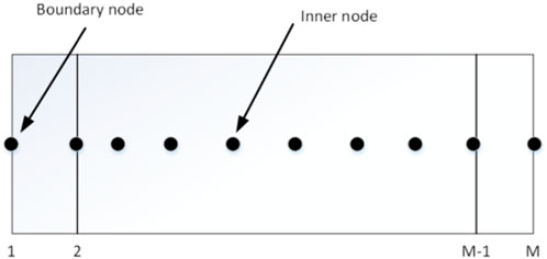
Figure 2. Mesh scheme of the heat structure.

Assuming that the thermal conductivity k and volumetric heat capacity $\rho C_p$ are constant, the difference equation of the m^th inner node can be expressed as (28) and the difference equations of boundary nodes can be expressed as (29) and (30).

${\rho }_m^{n+1}{C}_{p,m}^{n+1}\frac{T_m^{n+1}-T_m^n}{\Delta t}=k_m^{n+1}\frac{T_{m+1}^{n+1}-2T_m^{n+1}+T_{m-1}^{n+1}}{{\left(\Delta x\right)}^2}.(28)$

${\rho }_1^{n+1}{C}_{p,1}^{n+1}\frac{T_1^{n+1}-T_1^n}{\Delta t}=k_1^{n+1}\frac{T_2^{n+1}-2T_1^{n+1}}{{\left(\Delta x\right)}^2}.(29)$

${\rho }_M^{n+1}{C}_{p,M}^{n+1}\frac{T_M^{n+1}-T_M^n}{\Delta t}=k_M^{n+1}\frac{-2T_M^{n+1}+T_{M-1}^{n+1}}{{\left(\Delta x\right)}^2}.(30)$

2.2 Newton-based solution method

2.2.1 Basic solution procedure

The discrete process described above gives rise to a system of non-linear equations. To solve this system of discretized equations, the iterative Newton method (Süli and Mayers, 2003) is employed. The resulting set of equations can be expressed as follows:

$\frac{{\overrightarrow{y}}^{n+1}-{\overrightarrow{y}}^n}{\Delta t}=\overrightarrow{F}\left(t^{n+1},{\overrightarrow{y}}^{n+1}\right),(31)$

where

$\overrightarrow{F}\left(\overrightarrow{y}\right)={\left[f_1\left(\overrightarrow{y}\right),f_2\left(\overrightarrow{y}\right),\cdots ,f_n\left(\overrightarrow{y}\right)\right]}^{T.}(32)$

$\overrightarrow{y}={\left[y_1,y_2,\cdots ,y_n\right]}^T.(33)$

At the (k+1)-th iteration, it is possible to express the equation using a first-order Taylor expansion as follows:

$\overrightarrow{F}\left({\overrightarrow{y}}^{k+1}\right)\approx \overrightarrow{F}\left({\overrightarrow{y}}^k\right)+\frac{\partial \overrightarrow{F}}{\partial {\overrightarrow{y}}^k}\delta {\overrightarrow{y}}^k=0.(34)$

The linear system of Eq. 35 should be solved at each iteration, where $\frac{\partial \overrightarrow{F}}{\partial {\overrightarrow{y}}^k}$ is the Jacobian matrix and $\overrightarrow{F}\left({\overrightarrow{y}}^k\right)$ is the vector of residuals.

$\frac{\partial \overrightarrow{F}}{\partial {\overrightarrow{y}}^k}\delta {\overrightarrow{y}}^k=-\overrightarrow{F}\left({\overrightarrow{y}}^k\right).(35)$

The desired $\delta {\overrightarrow{y}}^k$ can be obtained by using the Gaussian elimination method. Then, we can get:

${\overrightarrow{y}}^{k+1}={\overrightarrow{y}}^k+\delta {\overrightarrow{y}}^k.(36)$

The flow chart of the Newton-based solution method is as demonstrated in Figure 3.

Figure 3

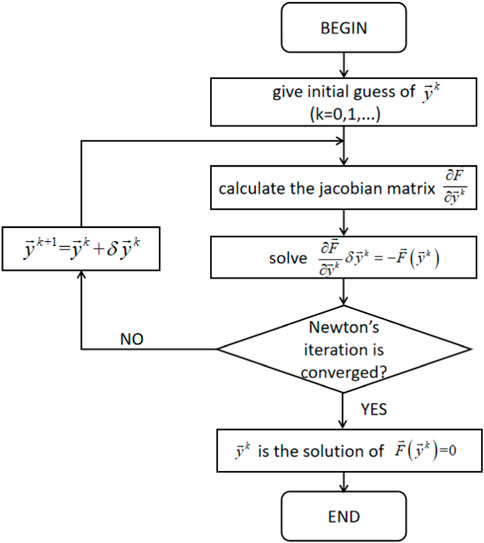
Figure 3. Flowchart of Newton’s iteration method.

The computational cost and memory for complex problems can be reduced by approximating the Jacobian matrix in Eq. 37 through a finite difference of the residuals, eliminating the need to explicitly construct the Jacobian matrix:

${\left(\frac{\partial \overrightarrow{F}}{\partial {\overrightarrow{y}}^k}\right)}_{ij}=\frac{\partial f_i}{\partial y_j}\approx \frac{f_i\left(y_1,y_2,\cdots ,y_j+\epsilon ,\cdots ,y_n\right)-f_i\left(y_1,y_2,\cdots ,y_j,\cdots ,y_n\right)}{\epsilon }.(37)$

The parameter $\epsilon$ is a perturbation parameter that is set to $1\times {10}^{-6}$ in this study.

2.2.2 Scaling modification technique

As mentioned above, the unknown variables in this study include steam mass, mass flow rate, and temperature. These variables may vary significantly in magnitude under certain operating conditions (for instance, in scenarios where steam content is low, the magnitude of steam mass may be approximately 0.01 or less, while in situations with high pressure differences, the magnitude of the mass flow rate may exceed thousands or more.). Such differences in magnitude among variables can affect the convergence and stability of Newton’s method described in Section 2.2.1. Therefore, special numerical methods are required.

The scaling modification technique is used to improve the convergence and stability of the algorithm. This involves scaling the variables by a certain factor to make their magnitudes more comparable. By applying variable scaling, Newton’s method can more effectively handle variables with different magnitudes, improving the convergence and stability of the algorithm.

Here are the steps to perform variable scaling:

1. Estimate the magnitudes of each variable.

2. Divide each variable by its estimated magnitude.

3. Apply the scaled variables in the iterations of Newton’s method.

4. Restore the final solution to the original variable magnitudes.

By applying the scaling modification technique, Newton’s method can adapt better to variables with different magnitudes, enhancing the efficiency and stability of the algorithm. This technique is particularly useful when dealing with ODEs in the containment analysis code and significant differences in unknown variable magnitudes (mass, mass flow rate, temperature, and some other variables) and can improve the convergence behavior of the method.

2.2.3 Line search method

To avoid divergence caused by the excessively long step size of Newton’s iteration method, the line search method is combined with Newton’s iteration method to improve its efficiency and convergence stability. The main idea of the line search method is to adjust the step size at each iteration to reduce the residual error of nonlinear equations.

In Newton’s method, the algorithm iteratively updates an initial guess for the solution by using the equation:

${\overrightarrow{y}}^{k+1}={\overrightarrow{y}}^k+\delta {\overrightarrow{y}}^k.(38)$

When applying the line search method, instead of using the above equation directly, the step size is scaled by a factor $\lambda$ as follows:

${\overrightarrow{y}}^{k+1}={\overrightarrow{y}}^k+\lambda \cdot \delta {\overrightarrow{y}}^k.(39)$

The purpose of the line search method is to make Newton’s method more robust and efficient by taking into account the decreased residual as follows:

$‖\overrightarrow{F}\left({\overrightarrow{x}}^{k+1}\right)‖\le ‖\overrightarrow{F}\left({\overrightarrow{x}}^k\right)‖.(40)$

It can improve the convergence rate, especially in cases where the initial guess is far from the solution.

By incorporating the line search method into Newton’s method, the algorithm can provide faster convergence and improved numerical stability, leading to more reliable results.

3 Application to typical stiff ODE problems

In this study, the proposed ODE solver was applied to some typical stiff ODE problems. The results of the computations were compared with the corresponding theoretical solutions or literature-derived values to verify that the solver is capable of solving the stiff ODE problems.

PROBLEM 1: To begin with, we consider an example of a stiff differential equation system that can be analytically solved, which is described in Eq. 41 as follows:

$\left\{\begin{array}{l}\frac{du}{dt}=-1000.25u+999.75v+0.5\\ \frac{dv}{dt}=999.75u-1000.25v+0.5\\ u\left(0\right)=1.0\\ v\left(0\right)=-1.0.\end{array}\right.(41)$

This set of equations has an analytical solution, as follows:

$\left\{\begin{array}{l}u\left(t\right)=-e^{-0.5t}+e^{-2000t}+1\\ v\left(t\right)=-e^{-0.5t}-e^{-2000t}+1.\end{array}\right.(42)$

The presence of the transient term $e^{-2000t}$ in the solution causes this system to be stiff. The profiles of u and v calculated by the proposed fully implicit solver, explicit Euler method, and explicit 4^th order Runge–Kutta method are compared with the analytical results, which are shown in Figures 4, 5. The figures above illustrate that these calculated values match the analytical solution very well. However, it is noteworthy that the explicit methods (Euler and RK methods) necessitate significantly smaller time steps compared to the fully implicit method. It is observed that when the time step of the explicit method is as large as that of the fully implicit method, the solutions are divergent. The computational results are illustrated in the figure below:

Figure 4

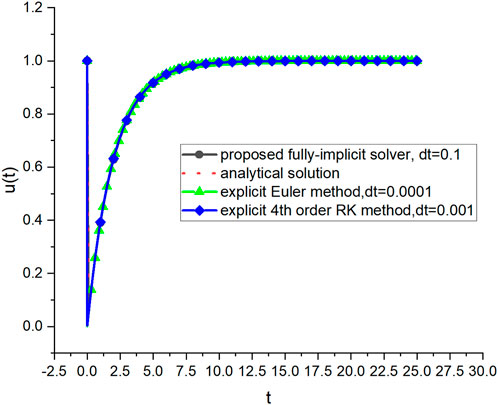
Figure 4. The time profile of u(t).

Figure 5

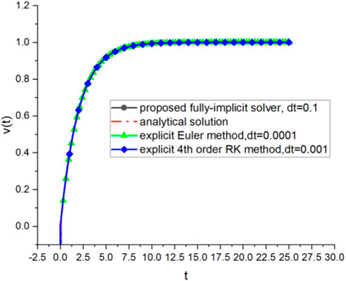
Figure 5. The time profile of v(t).

In addition, three different methods on a PC (13th Gen Intel(R) Core (TM) i9-13900H 2.60 GHz) were used to solve Eq. 41, and the total computational times required for the three methods are shown in Table 2. The result shows that the implicit method requires less overall computational effort compared to explicit methods.

Table 2

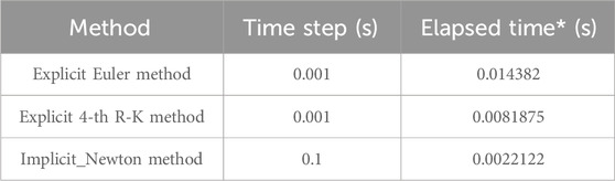
Table 2. Overall computational effort comparison among three solving methods.

PROBLEM 2: As described in Thohura and Rahman (2013), the following kinetics problem, originally proposed by Robertson, is commonly used as an illustrative instance in this field. The governing equations for this problem are described as follows:

$\left\{\begin{array}{l}\frac{d{y}_1}{dt}=-0.04y_1+{10}^4{y}_2{y}_3\\ \frac{d{y}_2}{dt}=0.04y_1-{10}^4{y}_2{y}_3-{3.10}^7{y}_2^2\\ \frac{d{y}_3}{dt}={3.10}^7{y}_2^2\\ y_1\left(0\right)=1.0\\ y_2\left(0\right)=0.0\\ y_3\left(0\right)=0.0.\end{array}\right.(43)$

Due to the long time span of this problem ($4\cdot {10}^{9}s\approx 126.755years$), the time steps for this problem are variable to finish this calculation, which is shown in Table 3.

Table 3

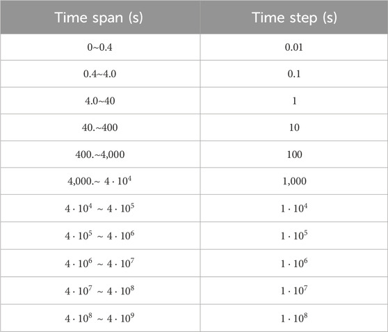
Table 3. Time steps used in problem 2.

As a result, only the calculated value of the proposed ODE solver and the literature-based value for this problem are compared, as shown in Figure 6. The results show that the calculated values agree well with values in the literature considering the long time span.

Figure 6

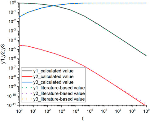
Figure 6. The comparison between the calculated value and literature-based value.

Consequently, the capabilities of the proposed ODE solver to solve stiff ODE equations are proven by these two typical stiff ODE equations.

4 Application in the containment T-H analysis

4.1 Application to the CNSI benchmark problem

As described in Haware et al. (1994), the CNSI benchmark problem consists of a single volume with injected steam and water, from which heat is transmitted to a single concrete wall. The nodalization of this problem is illustrated in Figure 7. The geometrical and thermal hydraulic parameters are listed in Table 4 and the mass flow rate profiles of injected water and steam are shown in Figure 8.

Figure 7

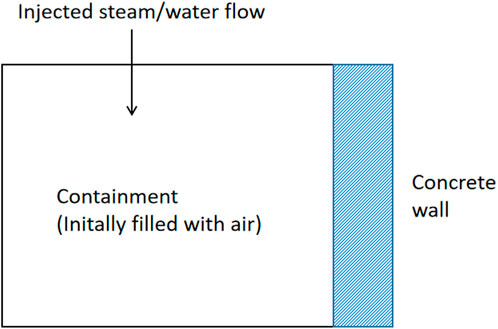
Figure 7. Nodalization of the CNSI benchmark problem.

Table 4

Table 4. Geometrical and thermal hydraulic parameters.

Figure 8

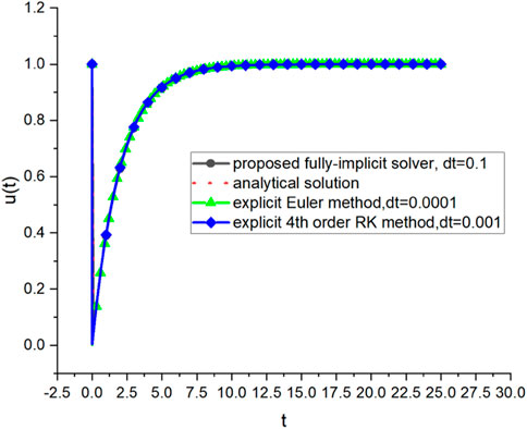
Figure 8. Injected water/steam mass flow rate.

An analytical solution for this benchmark problem was derived in Haware et al. (1994). Comparisons between calculated results and the analytical solution are shown in Figures 9, 10, 11. The total pressure in the containment volume is shown in Figure 9, the partial pressure of the steam is shown in Figure 10, and the wall surface temperature is shown in Figure 11.

Figure 9

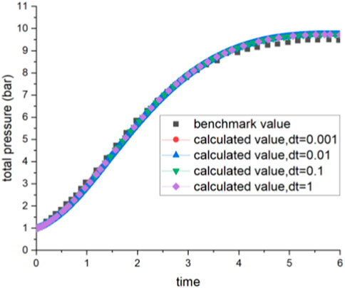
Figure 9. Comparison of total pressure between the benchmark and calculated value.

Figure 10

Figure 10. Comparison of steam pressure between the benchmark and calculated value.

Figure 11

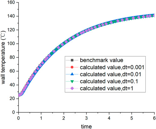
Figure 11. Comparison of temperature between the benchmark and calculated value.

The calculated results for all three parameters exhibit strong agreement with the analytical solution, providing evidence of the accuracy of the ODE-solver developed for the containment analysis code presented in this study. This ODE-solver effectively ensures the conservation of mass and energy within the fluid, as well as energy within the structural wall. Furthermore, the comparisons in Figures 9, 10 illustrate that both the calculated total pressure and steam partial pressure slightly exceed the benchmark value. This discrepancy can be attributed to the adoption of thermal non-equilibrium equations in this study, while the analytical solution is based on a thermal equilibrium model. The good agreement of the predicted wall surface temperature in Figure 11 indicates that the modeling of wall conduction is accurately represented in the analysis. In addition, Figure 9 to Figure 11 demonstrate that a larger time step (1 s) can yield the same results as a smaller time step. This observation substantiates the notion that the fully implicit method can, to a certain extent, alleviate the constraints imposed by the time step.

4.2 Application to the CVTR test 3 problem

A series of design basis accident (DBA) tests were conducted on the Carolinas Virginia Tube Reactor (CVTR) containment system (Norberg et al., 1969), and the pressure and temperature responses of the containment under steam injection were simulated. The configuration of the CVTR containment system is illustrated in Figure 12. The containment consists of a hemispherical dome and a cylindrical body, with a diameter of 17.68 m inside the cylindrical tube, a total height of approximately34.75 m, a wall thickness of approximately0.61 m, and a concrete wall structure, and a total free volume of the containment of approximately6425.66 m³. Depending on the height and function, the containment can be divided into four zones: the dome, the operation region, the intermediate region, and the basement region.

Figure 12

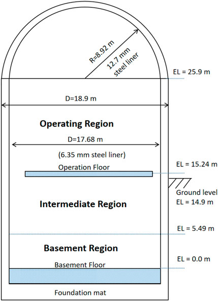
Figure 12. CVTR containment configuration.

Test 3 of CVTR, in which the spray system is not activated, is chosen to verify the thermal hydraulic analysis ability of the containment code with the proposed ODE solver. Only two nodes (the dome region and the containment main region) are simulated in this calculation without considering the inner connection of the compartments inside the containment, and the atmosphere environment is also simulated by a node, which is shown in Figure 13.

Figure 13

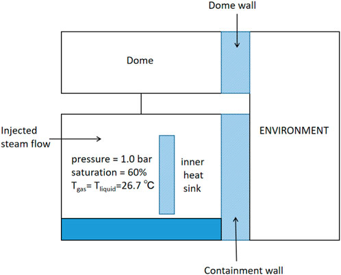
Figure 13. Nodalization of the CVTR containment.

The initial condition is also described in Figure 13, and the input parameters needed for the inner heat sink and containment wall are listed in Table 5. The mass flow rate and the enthalpy of injected steam are demonstrated in Figure 14.

Table 5

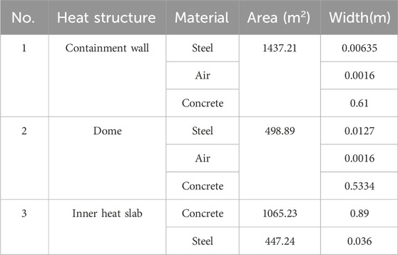
Table 5. The characteristic parameters of the heat structures in the CVTR containment.

Figure 14

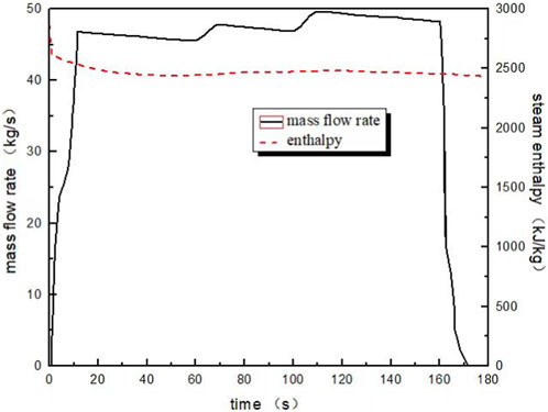
Figure 14. The mass flow rate and enthalpy of injected steam in CVTR test 3.

The comparison between the experimental and calculated values of pressure in the containment under test 3 conditions is shown in Figure 15. It can be seen in Figure 15 that the pressure inside the containment increases rapidly during the steam injection period and decreases slowly after the end of the steam injection, and the CASSIA code equipped with the proposed ODE solver is able to simulate this trend. The peak pressures calculated by the CASSIA code and those of the experimental values appear at basically the same time, but the peak pressure calculated by the CASSIA code is higher than the experimental value. The discrepancy can be attributed to the inadequate consideration of momentum-induced mixing phenomena in the initial pressurization process, as well as the fact that the correlation of the wall heat transfer coefficient used in the CASSIA code is conservative.

Figure 15

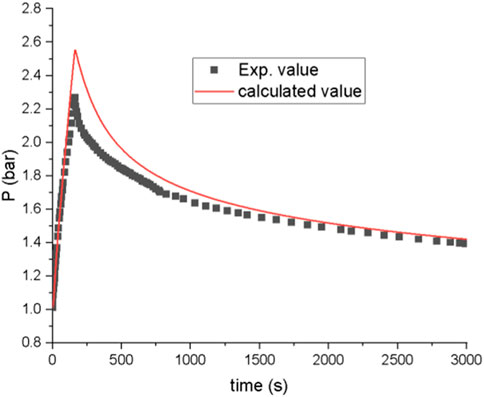
Figure 15. Comparison of pressure between the experimental value and the calculated value.

5 Conclusion

In this study, a general-purpose, fully implicit ODE solver for containment analysis code is developed.

The ODE solver uses a modified Newton iteration combined with scaling modification techniques and line search methods to improve its convergence and stability. The partial derivative components in the Jacobi matrix are calculated by the perturbation method using the finite difference approximation, which avoids the complicated derivation of partial derivatives.

This solver is employed to validate its efficacy in solving stiff ordinary differential equations (ODEs) by applying it to two representative cases. The calculated results for these two typical stiff ODE problems are subsequently compared against analytical solutions and literature-based values. The comparison results not only establish the proficiency of the proposed ODE solver in addressing stiff ODE equations but also illustrate its capability to handle calculations with significantly large time steps, as exemplified by problem 2.

Furthermore, the solver is also employed to assess its competence in conducting thermal–hydraulic analysis within a containment, specifically applied to the CNSI single-volume containment benchmark problem and CVTR test 3 problem. In the CNSI benchmark problem, three essential parameters, namely, total pressure, steam partial pressure, and wall temperature, are calculated. The obtained results for all three parameters exhibit a close agreement with the benchmark solution, thereby verifying the capability of the CASSIA code, which incorporates the developed ODE solver, to accurately calculate mass and energy conservation as well as wall heat conduction. In the CVTR test 3 problem, the pressure within the containment is compared to the experimental value. The observed trend and the timing of the peak pressure align closely with the experimental data, providing a preliminary assessment of the CASSIA code’s capability to conduct thermal hydraulic analysis within a containment.

It is worth noting that the Newton method adopted in the proposed ODE solver involves the computation of the Jacobian matrix, which can be computationally expensive, especially for large systems. Additionally, if the Jacobian needs to be updated in each iteration, it adds to the computational cost. Considering that the equations of the containment code are large and sparse, it may be beneficial to take advantage of the sparsity structure of the Jacobian matrix. Sparse matrix techniques can significantly reduce the computational cost of both storing and computing the Jacobian. This would be the future improvement of the proposed ODE solver.

Data availability statement

The raw data supporting the conclusion of this article will be made available by the authors, without undue reservation.

Author contributions

JH: methodology, software, and writing–original draft. JL: supervision and writing–review and editing. YM: software, validation, and writing–review and editing.

Funding

The author(s) declare that no financial support was received for the research, authorship, and/or publication of this article.

Acknowledgments

The authors would like to express their appreciation for the financial support of CNPRI (China Nuclear Power Technology Research Institute Co., Ltd.).

Conflict of interest

Authors JH, JL, and YM were employed by China Nuclear Power Technology Research Institute Co., Ltd.

The authors declare that this study received funding from China Nuclear Power Technology Research Institute Co., Ltd. The funder had the following involvement in the study: the decision to submit it for publication.

Publisher’s note

All claims expressed in this article are solely those of the authors and do not necessarily represent those of their affiliated organizations, or those of the publisher, the editors, and the reviewers. Any product that may be evaluated in this article, or claim that may be made by its manufacturer, is not guaranteed or endorsed by the publisher.

References

Allelein, H. J., Arndt, S., Klein-Hessling, W., Schwarz, S., Spengler, C., and Weber, G. (2008). COCOSYS: status of development and validation of the German containment code system. Nucl. Eng. Des. 238 (4), 872–889. doi:10.1016/j.nucengdes.2007.08.006

CrossRef Full Text | Google Scholar

Bogacki, P., and Shampine, L. F. (1989). A 3(2) pair of Runge–Kutta formulas. Appl. Math. Lett. 2, 321–325. doi:10.1016/0893-9659(89)90079-7

CrossRef Full Text | Google Scholar

Brosche, D. (1972). ZOCO V, a computer code for the calculation of time- and space-dependent pressure distributions in reactor containments. Nucl. Eng. Des. 23 (3), 239–271. doi:10.1016/0029-5493(72)90149-5

CrossRef Full Text | Google Scholar

Butcher, J. C. (2008). Numerical methods for ordinary differential equations. Chichester, UK: Wiley.

Google Scholar

Cai, Q., Fan, K., and Shan, J. (2022). Development and preliminary validation of fully implicit scheme single-phase liquid metal fast reactor code nusol-lmr. SSRN Electron. J., doi:10.2139/ssrn.4077541

CrossRef Full Text | Google Scholar

Chen, Y., Wu, Y. W., Wang, M. J., Zhang, Y., Tan, B., Zhang, D., et al. (2018). Development of a multi-compartment containment code for advanced PWR plant. Nucl. Eng. Des. 334, 75–89. doi:10.1016/j.nucengdes.2018.05.001

CrossRef Full Text | Google Scholar

Cooper, J. R., and Dooley, R. B. (2007). “Revised release on the IAPWS industrial formulation 1997 for the thermodynamic properties of water and steam,” in 18th International Conference on the Properties of Water and Steam, Boulder, Colorado, August, 2007.

Google Scholar

Florez, W. F., Gonzalez, J. W., Hill, A. F., López, J. D., and López, G. J. (2017). Numerical methods coupled with Richardson extrapolation for computation of transient power systems. Ing. Cienc. 13 (26), 65–89. doi:10.17230/ingciencia.13.26.3

CrossRef Full Text | Google Scholar

Gauntt, R., Cole, R., Erickson, C., Gido, R., Gasser, R., Rodriguez, S., et al. (2005). MELCOR computer code manuals. Albuquerque, New Mexico: Sandia National Laboratories, 6119. NUREG/CR.

Google Scholar

George, T. L., Wiles, L., Claybrook, S., Wheeler, C., and McElroy, J. (2001). Gothic containment analysis package technical manual. Richland, WA, USA: Numerical Applications Inc.

Google Scholar

Hairer, E., and Wanner, G. (1989). Stiff differential equations solved by Radau methods. J. Compu. Appl. Math. 111, 93–111. doi:10.1016/s0377-0427(99)00134-x

CrossRef Full Text | Google Scholar

Haware, S. K., Ghosh, A. K., Raj, V. V., and Kakodkar, A. (1994). “Analysis of CSNI benchmark test on containment using the code CONTRAN,” in Proceedings of the third international conference on containment design and operation v2, Canada, 580.

Google Scholar

Hoffman, J. D., and Frankel, S. (2001). “Fixed-point iteration,” in Numerical methods for engineers and scientists (New York, NY, USA: CRC Press), 141–145.

Google Scholar

Merga, F. E., and Chemeda, H. M. (2021). Modified crank–nicolson scheme with Richardson extrapolation for one-dimensional heat equation. Iran. J. Sci. Technol. Transaction A, Sci. 45 (54), 1725–1734. doi:10.1007/s40995-021-01141-0

CrossRef Full Text | Google Scholar

Moran, M., and Shapiro, H. (1992). Fundamentals of engineering thermodynamics. SERBIULA (sistema librum 2.0). Available at: http://ftp.demec.ufpr.br/disciplinas/TM104/Termodinamica/Moran-Thermo-Book/Michael%20J.%20Moran,%20Howard%20N.%20Shapiro,%20Daisie%20D.%20Boettner,%20Margaret%20B.%20Bailey%20-%20Fundamentals%20of%20Engineering%20Thermodynamics%20(2014,%20Wiley).pdf

Google Scholar

Murata, K., Williams, D., Griffith, R., Gido, R., Tadios, E., Davis, F., et al. (1997). Code manual for CONTAIN 2.0: a computer code fornuclear reactor containment analysis, Albuquerque, NM, UnitedStates: Nuclear Regulatory Commission, Washington,DC (United States). Div. of Systems Technology; Sandia National Labs., Albuquerque,NM (United States); Tills (Jack) and Associates, Inc.,

Google Scholar

Norberg, J. A., Bingham, G. E., and Schmitt, R. C. (1969). Simulated design basis accident tests of the Carolinas Virginia tube reactor containment: preliminary results. Denton, Texas: UNT Digital Library. doi:10.2172/4753505

CrossRef Full Text | Google Scholar

O'Dell, C R, and Wong, K (2010). COCOSYS – New Modelling of Safety Relevant Phenomena and Components. Heling 111, 846.

Google Scholar

Press, W. H., Teukolsky, S. A., Vetterling, W. T., and Flannery, B. P. (2007). Numerical recipes: the art of scientific computing. Cambridge, United Kingdom: Cambridge University Press.

Google Scholar

Süli, E., and Mayers, D. (2003). An introduction to numerical analysis. Cambridge, United Kingdom: Cambridge University Press.

Google Scholar

Tagami, T. (1965). Interim report on safety assessment and facilities establishment project in Japan for period ending. NUREG-75/087. National Reactor Testing Station.

Google Scholar

Thohura, S., and Rahman, A. (2013). Numerical approach for solving stiff differential equations: a comparative study. Glob. J. Sci. Front. Res.,

Google Scholar

Uchida, H., Oyama, A., and Togo, Y. (1964). Evaluation of post-incident cooling systems of light-water power reactors. A/CONF.28/P/436. Tokyo: Tokyo Univ.,

Google Scholar

Wille, D. R. (1998). Experiments in stepsize control for Adams linear multistep methods. Adv. Comput. Math. 8 (4), 335–344. doi:10.1023/a:1018960717197

CrossRef Full Text | Google Scholar

Yuan, Y. (2000). “A review of trust region algorithms for optimization,” in Iciam 99: proceedings of the fourth international congress on industrial and applied mathematics, edinburgh (USA: Oxford University Press).

CrossRef Full Text | Google Scholar

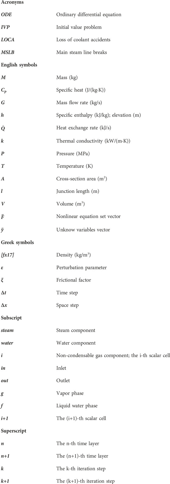
Nomenclature