Transient synchronization stability of photovoltaics integration by singular perturbation analysis

The integration of large-scale photovoltaics (PVs) into the power grid has significantly altered the transient synchronization dynamics of traditional power systems dominated by synchronous generators (SGs) and posed great challenges to modeling and analysis of PVs integration. In this paper, the transient synchronization stability of the PV-SG system is studied using the singular perturbation technique. Firstly, a nonlinear model of a PV-SG system is established to reveal the multiscale transient synchronization characteristics. Further, the full system is decomposed into a slow subsystem and a fast subsystem by the singular perturbation technique. The fast subsystem containing the dynamics of the DC voltage control, terminal voltage control, and phase-locked loop, and the slow subsystem containing the dynamics of rotor motion can perfectly reflect the dynamics of the full system within the electromagnetic and electromechanical timescales, respectively. The proposed model provides a clearer physical picture of dynamics in the PV-SG system within the electromagnetic and electromechanical timescales. Subsequently, the stability of the slow and fast subsystems is investigated using the energy function and eigenvalue analysis methods, respectively. Meanwhile, the impacts of various operating, control, and structural parameters on the transient synchronization stability are uncovered. Different from the most existing research endeavors on the wide simulations of the PVs integration, the impact of PVs on the synchronization dynamics of SGs without considering the dynamical characteristics of the PV system, and the transient synchronization stability analyses of the PLL-based voltage source converter systems, it is the key contribution to study the transient synchronization dynamical characteristics of the PV system and its interaction with the SG under different timescales. All these are helpful and easy to extend to more complicated PV-SG systems. Finally, the analysis results are validated by extensive simulations.

1 Introduction

The integration of large-scale photovoltaics (PVs) into the grid has significantly altered the dynamics of traditional power systems dominated by synchronous generators (SGs). It has brought great impacts and challenges to the modeling and analysis of power systems integrated with PVs (Shah et al., 2015; Kabeyi and Olanrewaju, 2022; Xiong et al., 2022). PVs are connected to the grid through power electronic equipment. The transient characteristics with PV integration differ significantly from those of traditional power systems, and the transient stability issues are increasingly prominent (Gandhi et al., 2020; He H. et al., 2022; Seane et al., 2022). It has been reported that a phase-to-phase fault of a 500 kV transmission line in California resulted in an approximately 900 MW PV off-grid, with one of the primary causes being the loss of synchronization (NERC Joint and WECC Staff, 2018). Hence, it is urgent to uncover the transient synchronization mechanism for the power systems integrated with PVs.

Voltage source converter (VSC) is a fundamental component of power electronic equipment, and its dynamical behaviors are primarily dominated by control units, which differ significantly from those of SGs dominated by the rotor motion (Wang et al., 2020; Chen et al., 2023). The rotor motion is represented by the second-order swing equation within the electromechanical timescale (Kundur, 1994). For the transient stability analysis of power-electronic-dominated power systems, several approaches have been developed, including the time-domain simulation (Zhao et al., 2021), energy function (Zhang et al., 2022), equal-area criterion (Xu et al., 2023), phase portrait (Wu and Wang, 2020), hyperplane method (Ma et al., 2023a), basin of attraction (Zhang et al., 2020), and bifurcation analysis (Ma et al., 2022a). Usually, the transient synchronization of the VSC grid-tied systems belongs to the electromagnetic timescale, including the DC voltage control timescale and AC current control timescale (Yuan et al., 2017; Ma et al., 2023b). Corresponding models for the single-VSC system have been developed in (Ma et al., 2020; Yang et al., 2020).

There are already several studies on the transient stability analysis of power systems integrated with the PVs. The response of the relative rotor angle is investigated in a large-scale system with the PV penetration levels of 0% and 20% under three-phase faults (Eftekharnejad et al., 2013). It has been found that the impact of PV integration depends on the system topology, PV penetration levels, fault types, and fault locations as well. Based on the Texas 2000-bus system, the effects of large-scale PVs on the transient stability are studied (Kumar et al., 2019). As demonstrated, the benefits of PV integration are strongly related to the factors such as the node criticality, type, location and penetration of PVs, as well as types of transients. The impacts on the transient stability are analyzed in the 39-bus and 118-bus systems, under different grounding fault locations and various reactive power control strategies (Rezaei et al., 2022). It is found that they depend on the disturbance types, PV installation locations, and network structure. The impact of PV penetration level on the transient stability of Ontario power system is also assessed and it is demonstrated that distributed PVs can considerably improve system stability (Tamimi et al., 2013). An online transient stability assessment criterion is proposed for the grid-connected PV generator by monitoring the energy swing of the dc link capacitor (Priyamvada and Das, 2020a; Priyamvada and Das, 2020b). In Hossain and Ali (2015), three nonlinear controllers are proposed to enhance the transient stability of a large-scale hybrid power system. By making the PV inverter’s dc link capacitors absorb some of the SG kinetic energy, novel control schemes for PV inverters are also proposed in (Zevallos et al., 2021; Landera et al., 2022), to improve the transient stability of the SG in the radial and meshed power systems, respectively. However, most of these studies are based on simulations, making it difficult to provide mechanistic explanations for the transient stability of power systems integrated with PVs in general.

On the other hand, for the mechanistic analysis of the transient synchronization stability, many studies focus on the phase-locked loop based (PLL-based) VSC systems. In addition, recently a detailed model for the multi-machine PV-SG power systems is established in (Pico and Johnson, 2019), but its application is difficult due to its complexity. By neglecting the PLL dynamics and accounting for the algebraic constraints caused by the existence of its equilibrium point, the impact of the VSC on the transient stability of the SG is investigated in He and Geng (2021). Based on their respective synchronization loops, a second-order model for the relative angle and frequency is developed and a unified stability criterion is proposed in (He C. et al., 2022). The interaction term of two VSCs is modeled and the equal area criterion is adopted to study the transient synchronization stability of the two-VSC grid-connected system (Fu et al., 2022; He and Geng, 2022). Further, a dual-iteractive equal area criterion is proposed in Li et al. (2023). A mathematical model of the paralleled VSC and virtual synchronous generator is established and the transient synchronization stability is studied based on extended equal area criterion theory and Lyapunov’s function (Shen et al., 2021). Nevertheless, these studies mainly focus on the synchronization loop PLL and ignore the outer control loops. A clear picture of transient synchronization characteristics, modeling, and stability with PVs integration still lacks.

To address the aforementioned challenging issues, the singular perturbation technique is used to investigate the transient synchronization stability of the PV-SG system. The main contributions of the paper are summarized as follows:

1) By utilizing the singular perturbation technique, we divide the full system into two slow and fast subsystems, which reflect the electromechanical and electromagnetic timescale dynamics, respectively. The proposed model offers a clearer physical picture for the PV-SG system dynamics and the interactions between the PV system and the SG under different timescales become clearer.

2) Based on the reduced-order slow and fast subsystems, the transient synchronization stability analysis of the full system is studied and the parameter impacts on the stability are uncovered.

The paper is organized as follows. In Section 2, a nonlinear model for the PV-SG system is established and its transient synchronization characteristics are revealed. In Section 3, by employing the singular perturbation technique, the multi-timescale decomposition is carried out to divide the full system into two independent slow and fast subsystems. In Section 4, the stability of the slow and fast subsystems is analyzed by using the energy function and eigenvalue analysis methods, and the impacts of various parameters on stability are uncovered. In addition, Section 5 conducts extensive electromagnetic transient (EMT) simulations with the aid of MATLAB/Simulink, which verifies the validity of the analytical results. Finally, conclusions and discussions are presented in Section 6.

Here, we would like to emphasize that in our recent conference paper (Wu et al., 2023), the singular perturbation technique has been used to model the multi-machine power systems integrated with PVs. The multi-machine model in Wu et al. (2023) clarifies variable relations between the equipment and network, and lays a foundation for some further stability analyses. Here, in this paper, we mainly focus on the interactions between the PV system and the SG under different timescales and perform the transient synchronization stability analysis.

2 Nonlinear modeling of the PV-SG system

2.1 Control scheme and model assumptions

Figure 1 shows the circuit topology and control block diagram of the PV-SG parallel system. The single-stage PV array is connected to the system through the VSC, connected in parallel with the SG and then connected to the infinite grid. The PV grid-tied system adopts the vector control scheme, comprising the outer loop voltage control, alternating current control (ACC), and phase-locked loop (PLL) control. The linear proportional-integral (PI) controllers are adopted, which have been widely used in industrial control systems. The outer loop voltage control includes the DC voltage control (DVC) and the terminal voltage control (TVC). For the single-stage PV grid-tied system, the maximum power point tracking (MPPT) control regulates the DC voltage reference to operate at the maximum power-point based on the output current and the DC voltage of the PV array as well as inherent algorithms. Common MPPT algorithms include the perturb and observe algorithm and the incremental conductance algorithm. By comparing the DC voltage and the terminal voltage with their corresponding references, the current references in the dq reference frame are obtained. Then, the ACC compares the current references with their actual values to generate the voltage references in the dq reference frame. Moreover, the output angle of the synchronization loop PLL is used for the coordinate transformation to obtain the voltage references in the xy reference frame. Subsequently, the voltage references are modulated to control the switching states of the six insulated gate bipolar transistors (IGBTs) by the pulse width modulation technique.

FIGURE 1

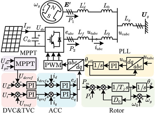
FIGURE 1. Schematic show of the PV-SG parallel system and its controls.

For modeling, the SG adopts the classical second-order model and can be represented as a constant transient potential connected to the network through a transient inductance $L_d^{\prime }$. Since the ACC is much faster than the outer loop voltage control and PLL control, the dynamics of the ACC are ignored. It is assumed that the output current values of the PV system can simultaneously track their respective reference values in the dq reference frame, i.e., i_d = i_dref and i_q = i_qref. Furthermore, the dynamics of the inductors are neglected, and the network is described by the phasor model. Usually, the change of environmental temperature and irradiance is a relatively slow process, so it is not considered in the transient analysis. The MPPT control of the PV system is also not taken into account, meaning that the reference value of the DC side remains constant under the given external environmental conditions. The VSC is modeled by the average model, and the converter losses and line resistance are also neglected. Under these assumptions, the SG can be treated as a voltage source, while the PV system can be regarded as a controlled current source. The control diagram of the PV-SG parallel system can be redrawn in Figure 2. X₁ is defined as the sum of the transient reactance $X_d^{\prime }$ of the SG $(X_d^{\prime }={\omega }_0{L}_d^{\prime })$ and the reactance X₀ of the connected line (X₀ = ω₀L₀). X₂ represents the equivalent line reactance of the PV integration (X₂ = ω₀L₂) and X_g represents the grid reactance (X_g = ω₀L_g). Here, ω₀ represents the working frequency.

FIGURE 2

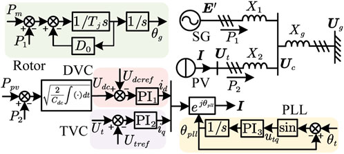
FIGURE 2. Schematic show of the redrawn control block diagram of the PV-SG parallel system under some simplifications.

The phase relations between the xy reference frame and the dq reference frame are shown in Figure 3. The vector in the xy reference frame is represented by a bold variable, such as U = u_x + ju_y = Ue^jθ, where u_x and u_y are the xy components of U. U and θ denote the amplitude and phase of U, respectively. The bold variable with the superscript “c” denotes the vector in the dq reference frame, such as U^c = u_d + ju_q, where u_d and u_q are the dq components of U^c. The xy reference frame rotates at a fundamental speed ω₀, with the x-axis aligned with the voltage vector U_g of the infinite grid. The dq reference frame rotates at a variable speed ω_pll, and the angle difference between the dq reference frame and xy reference frame is θ_pll. The voltage vector E′ of the SG rotates at a variable speed ω_g, and its phase in the xy reference frame is θ_g.

FIGURE 3

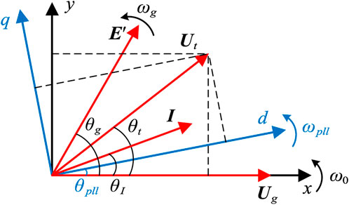
FIGURE 3. Schematic show of the xy reference frame, rotating at the fundamental speed ω₀, and dq reference frame, rotating at the variable speed ω_pll.

2.2 Modeling of the SG

The SG adopts the classical model and can be represented as a voltage source connected to the network through a transient reactor. The amplitude E′ of the voltage source is constant. The dynamics of the rotor angle are represented by the second-order swing equation:

$\left\{\begin{array}{c}{\dot{\theta }}_g=\left({\omega }_g-1\right){\omega }_o\hfill \\ T_j{\dot{\omega }}_g=P_m-P_1-D_0\left({\omega }_g-1\right)\hfill \end{array}\right.(1)$

where θ_g and ω_g denote the rotor angle and angular speed, respectively, P_m and P₁ represent the mechanical power and electromagnetic power, respectively, and T_j and D₀ are the inertial time constant and damping, respectively. Note that P₁ should be obtained from the network.

2.3 Modeling of the PV grid-tied system

2.3.1 PV array

The PV array adopts the commonly used model in engineering (Villalva et al., 2009; Liu et al., 2011). The output current of the PV array is a nonlinear function on the DC voltage, that is,

$I_{pv}=I_{sc}-C_1{I}_{sc}\left(e^{U_{dc}/\left(C_2{U}_{oc}\right)}-1\right)(2)$

where $C_1=\left(1-I_{\mathit{mpp}}/I_{sc}\right)e^{-U_{\mathit{mpp}}/\left(C_2{U}_{oc}\right)}$ and $C_2=\left(U_{\mathit{mpp}}/U_{oc}-1\right){\left[\ln \left(1-I_{\mathit{mpp}}/I_{sc}\right)\right]}^{-1}$. U_oc, I_sc, U_mpp, and I_mpp are the open-circuit voltage, short-circuit current, and voltage and current at the maximum power point of the PV array, respectively.

Thus, the output power of the PV array becomes a nonlinear function of U_dc,

$P_{pv}=U_{dc}\left(I_{sc}-C_1{I}_{sc}\left(e^{U_{dc}/\left(C_2{U}_{oc}\right)}-1\right)\right)(3)$

2.3.2 VSC

The standard form of the PI controller, with u(t) as the input and y(t) as the output, is represented as

$y\left(t\right)=K_p\left[u\left(t\right)+\frac{1}{\tau }{\int }_0^{t}u\left(t\right)dt\right](4)$

where the integral time constant τ = K_p/K_i, and K_p and K_i are the proportional and integral coefficients of the PI controller, respectively.

Selecting the state variable x as the output of the integrator:

$x\left(t\right)=\frac{1}{\tau }{\int }_0^{t}u\left(t\right)dt(5)$

yields

$\left\{\begin{array}{c}\dot{x}\left(t\right)=u\left(t\right)/\tau \hfill \\ y\left(t\right)=K_p\left(u\left(t\right)+x\left(t\right)\right)\hfill \end{array}\right.(6)$

1) DVC & TVC: Let the state variables x₁ and x₂ denote the output of the integrators in the DVC and TVC, respectively, we have their differential equations:

$\left\{\begin{array}{c}{\dot{x}}_1=\left(U_{dc}-U_{\mathit{dcref}}\right)/{\tau }_1\hfill \\ {\dot{x}}_2=\left(U_t-U_{\mathit{tref}}\right)/{\tau }_2\hfill \end{array}\right.(7)$

Correspondingly, the output currents are represented by the algebraic equations

$\left\{\begin{array}{c}{i}_d=K_{p1}\left(U_{dc}-U_{\mathit{dcref}}+x_1\right)\hfill \\ i_q=K_{p2}\left(U_t-U_{\mathit{tref}}+x_2\right)\hfill \end{array}\right.(8)$

where U_t is obtained from the network.

2) PLL: The PLL comprises an integrator and a PI controller. The x₃ represents the output of the integrator in the PI controller, and the corresponding differential equations are

$\left\{\begin{array}{c}{\dot{x}}_3=\sin \left({\theta }_t-{\theta }_{\mathit{pll}}\right)/{\tau }_3\hfill \\ {\dot{\theta }}_{\mathit{pll}}=K_{p3}\left(\sin \left({\theta }_t-{\theta }_{\mathit{pll}}\right)+x_3\right)\hfill \end{array}\right.(9)$

where θ_t is also obtained from the network.

3) Dynamics of the DC capacitor: The mismatch between the input and the output powers is the derivative of the energy on the DC capacitor, namely,

${\dot{U}}_{dc}=\frac{P_{pv}-P_2}{C_{dc}{U}_{dc}}(10)$

where the output electromagnetic active power P₂ of the PV system is obtained from the network.

In addition, the amplitude and phase of the output current vector I can be derived as

$\left\{\begin{array}{c}I=\sqrt{i_d^2+i_q^2}\hfill \\ {\theta }_I={\varphi }_I+{\theta }_{\mathit{pll}}\hfill \end{array}\right.(11)$

where ϕ_I denotes the phase in the dq reference frame of the current vector I. ϕ_I = arctan (i_q/i_d).

2.4 Modeling of the terminal voltage and active powers

Based on the superposition theorem on the circuit in Figure 2 including the three branches: 1) an infinite bus U_g with a series X_g, 2) a transient potential E′ with a series X₁, and 3) a current source I from the PV system, the parallel bus voltage vector U_c of the SG and the PV system can be obtained by

$U_c{e}^{j{\theta }_c}=K_1{U}_g{e}^{j0}+K_2{E}^{\prime }{e}^{j{\theta }_g}+j{X}_{3}I{e}^{j{\theta }_I}(12)$

where K₁ = X₁/(X₁ + X_g), K₂ = X_g/(X₁ + X_g), and X₃ = X₁X_g/(X₁ + X_g).

The output electromagnetic active powers of the SG and the PV system can be derived as

$\left\{\begin{array}{c}{P}_1=E^{\prime }{U}_g\sin {\theta }_g/\left(X_1+X_g\right)-K_2{E}^{\prime }I\cos \left({\theta }_g-{\theta }_I\right)\hfill \\ P_2=K_1{U}_{g}I\cos {\theta }_I+K_2{E}^{\prime }I\cos \left({\theta }_g-{\theta }_I\right)\hfill \end{array}\right.(13)$

The xy components of the terminal voltage vector U_t of the PV system is

$\left\{\begin{array}{c}{u}_{tx}=K_1{U}_g+K_2{E}^{\prime }\cos {\theta }_g-\left(X_2+X_3\right)I\sin {\theta }_I\hfill \\ u_{ty}=K_2{E}^{\prime }\sin {\theta }_g+\left(X_2+X_3\right)I\cos {\theta }_I\hfill \end{array}\right.(14)$

Thus, the amplitude and phase of the terminal voltage vector U_t can be obtained:

$\left\{\begin{array}{c}{U}_t=\sqrt{u_{tx}^2+u_{ty}^2}\hfill \\ {\theta }_t=\arctan \left(u_{ty}/u_{tx}\right)\hfill \end{array}\right.(15)$

2.5 Bulk transient synchronization characteristics of the PV-SG system

The dynamics of the SG are dominated by the rotor motion and its transient synchronization process belongs to the electromechanical timescale. In contrast, the PLL provides the reference angle between the dq and xy reference frames, and its electromagnetic timescale dynamics are dominant. The synchronization of the PV-SG system can be regarded as the synchronization between the state variables of the rotor angle θ_g and the PLL output angle θ_pll (Ma et al., 2023c; Zhang et al., 2023). From (11), (14), and (15), it becomes evident that the magnitude U_t and phase θ_t of the terminal voltage vector of the PV system depend on the variables θ_g, i_d, i_q, and θ_pll. As a result, the control diagram of the PV-SG system is illustrated in Figure 4A, where the functions f₁ and f₂ are determined by (11), (14), and (15).

FIGURE 4

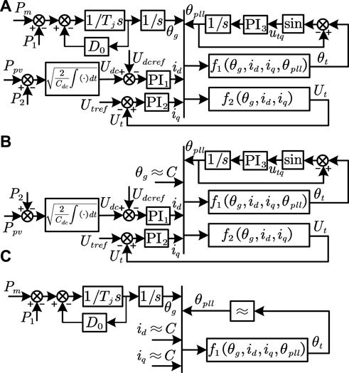
FIGURE 4. Schematic shows of the control diagram of the PV-SG parallel system for (A) the whole transient process, (B) in the early stage after the fault, and (C) after hundreds of milliseconds.

When a fault occurs, the PV-SG system experiences a sequence of changes. Here, we divide the whole process into three stages for a stable case. In stage I, the rotor angle θ_g is essentially unchanged in the early stage. The transient behaviors of the PLL output angle θ_pll are dominated by the dynamics of the DVC, TVC, and PLL, showing electromagnetic timescale dynamics, as shown in Figure 4B. In stage II, after hundreds of milliseconds, the response of electromagnetic timescale dynamics of the PV system finishes. The DC voltage, terminal voltage, and PLL output angle essentially equal to their corresponding reference values, i.e., U_dc ≈ U_dcref, U_t ≈ U_tref, θ_pll ≈ θ_t. Thus, the output currents i_d and i_q remain essentially unchanged. At this point, the transient behaviors are dominated by the swing equation of the SG, showing electromechanical timescale dynamics in a long term, as shown in Figure 4C. Finally, in stage III, the response of electromechanical timescale dynamics of the SG finishes and the system reaches a steady state again.

Consequently, the transient synchronization processes of the PV-SG system show multi-timescale dynamics. The rotor angle θ_g of the SG consistently performs electromechanical timescale dynamics, whereas the PLL output angle θ_pll belongs to the electromagnetic timescale and is dominant in the early stage of the fault. Subsequently, the electromagnetic timescale dynamics of the PLL output angle θ_pll rapidly attenuate. The long-term behavior of the rotor angle θ_g is dominant and the PLL output angle θ_pll also becomes the electromechanical timescale.

3 Reduced-order model

3.1 Introduction of singular perturbation theory

According to the theory of integral manifolds, the singular perturbation technique can be applied to analyze multi-timescale characteristics in nonlinear dynamics. Essentially, it replaces the integral manifold of a high-dimensional system with the integral manifold of a low-dimensional system, and thus decomposes the full system into two fast and slow subsystems (Shchepakina et al., 2014).

A standard singular perturbed system is

$\left\{\begin{array}{c}\dot{\mathbf{X}}=\mathbf{f}\left(\mathbf{X},\mathbf{Y},\epsilon \right)\hfill \\ \epsilon \dot{\mathbf{Y}}=\mathbf{g}\left(\mathbf{X},\mathbf{Y},\epsilon \right)\hfill \end{array}\right.(16)$

where X and Y are the slow and fast variables, $\mathbf{X}\in {\mathbb{R}}^m$, and $\mathbf{Y}\in {\mathbb{R}}^n$ ɛ denotes a small positive parameter, and 0 < ɛ ≪ 1.

Let ɛ = 0 in (16), we have the slow subsystem

$\left\{\begin{array}{c}\dot{\mathbf{X}}=\mathbf{f}\left(\mathbf{X},\mathbf{Y},0\right)\hfill \\ 0=\mathbf{g}\left(\mathbf{X},\mathbf{Y},0\right)\hfill \end{array}\right.(17)$

The timescale transformation is performed by taking τ = t/ɛ in (16) to derive the fast subsystem. Then, the equivalent singular perturbation system can be written as

$\left\{\begin{array}{c}{\mathbf{X}}^{\prime }=\mathbf{d}\mathbf{X}/\mathbf{d}\tau =\epsilon \mathbf{f}\left(\mathbf{X},\mathbf{Y},\epsilon \right)\hfill \\ {\mathbf{Y}}^{\prime }=\mathbf{d}\mathbf{Y}/\mathbf{d}\tau =\mathbf{g}\left(\mathbf{X},\mathbf{Y},\epsilon \right)\hfill \end{array}\right.(18)$

Similarly, by setting ɛ = 0 in (18), the fast subsystem can be derived:

$\left\{\begin{array}{c}{\mathbf{X}}^{\prime }=0\hfill \\ {\mathbf{Y}}^{\prime }=g\left(\mathbf{X},\mathbf{Y},0\right)\hfill \end{array}\right.(19)$

By utilizing the singular perturbation technique, the full system can be reduced to two independent fast and slow subsystems. By their stability analyses, the stability of the full system can be assessed. Only when both the fast and slow subsystems are stable, the full system is stable (Khalil, 2002). The full PV-SG system can be represented by a set of nonlinear differential algebraic equations. Therefore, according to the time constants of the state variables in the differential equations, we can perform the timescale decomposition to derive the corresponding fast and slow subsystems.

3.2 Slow subsystem

According to (1), (7), (9), and (10), we have the differential equations of the full system:

$\left\{\begin{array}{c}{\tau }_1{\dot{x}}_1=U_{dc}-U_{\mathit{dcref}}\hfill \\ {\tau }_2{\dot{x}}_2=U_t-U_{\mathit{tref}}\hfill \\ {\tau }_3{\dot{x}}_3=\sin \left({\theta }_t-{\theta }_{\mathit{pll}}\right)\hfill \\ {\tau }_{\mathit{pll}}{\dot{\theta }}_{\mathit{pll}}=\sin \left({\theta }_t-{\theta }_{\mathit{pll}}\right)+x_3\hfill \\ {\tau }_C{\dot{U}}_{dc}=P_{pv}-P_2\hfill \\ {\tau }_4{\dot{\theta }}_g=\left({\omega }_g-1\right){\omega }_o\hfill \\ {\tau }_5{\dot{\omega }}_g=P_m-P_1-D_0\left({\omega }_g-1\right)\hfill \end{array}\right.(20)$

Take the parameters in Supplementary Material S1, we have τ₁ = K_p1/K_i1 = 0.025 s, τ₂ = K_p2/K_i2 = 0.01 s, τ₃ = K_p3/K_i3 = 0.025 s, τ_pll = 1/K_p3 = 0.02 s, τ_C = C_dc = 0.1 s, τ₄ = 1 s, and τ₅ = T_j = 5 s. The values of τ₁, τ₂, τ₃, τ_pll, and τ_C are between 0.01 s and 0.1 s, while τ₄ and τ₅ are between 1 s and 10 s. Thus, x₁, x₂, x₃, θ_pll, and U_dc (for the PV system) are fast variables, and θ_g and ω_g (for the SG) are slow variables.

Setting τ₁, τ₂, τ₃, τ_pll, τ_C = 0 in (20), we have the second-order differential equations of the slow subsystem:

$\left\{\begin{array}{c}{\tau }_4{\dot{\theta }}_g=\left({\omega }_g-1\right){\omega }_o\hfill \\ {\tau }_5{\dot{\omega }}_g=P_m-P_1-D_0\left({\omega }_g-1\right)\hfill \end{array}\right.(21)$

The differential equations for the fast variables in the full system degenerate into the algebraic equations:

$\left\{\begin{array}{c}{U}_{dc}=U_{\mathit{dcref}},U_t=U_{\mathit{tref}}\hfill \\ u_{tq}=0,{\theta }_t={\theta }_{\mathit{pll}}\hfill \\ P_2=P_{pv}\hfill \end{array}\right.(22)$

It can be found that the fast variables quickly follow their corresponding reference values during the transient processes. Therefore, the output characteristics of the PV system shift from a controlled current source to an active power source (P_pv) with a constant voltage magnitude (U_tref), as P₂ = P_pv and U_t = U_tref. Meanwhile, the dynamics of the slow subsystem are dominated by the rotor swing equation within the electromechanical timescale.

In order to better handle the interface relations between the SG, the PV system, and the network within the electromechanical timescale, the output of the PV system is treated as a voltage vector with a current vector as its input. Applying the superposition theorem again on the modified circuit in Figure 2 including the three branches: 1) an infinite bus U_g with a series X_g, 2) a transient potential E′ with a series X₁, and 3) a voltage source U_t with a series X₂ from the PV system, the voltage vector U_c can be derived:

$U_c{e}^{j{\theta }_c}=K_1^{\prime }{U}_g{e}^{j0}+K_2^{\prime }{E}^{\prime }{e}^{j{\theta }_g}+K_3^{\prime }{U}_t{e}^{j{\theta }_t}(23)$

where $K_1^{\prime }=(X_1//X_2)/(X_g+X_1//X_2)$, $K_2^{\prime }=(X_2//X_g)/(X_1+X_2//X_g)$, and $K_3^{\prime }=(X_1//X_g)/(X_2+X_1//X_g)$.

The output electromagnetic active power of the SG can be further obtained by

$P_1=K_1^{\prime }{E}^{\prime }{U}_g\sin {\theta }_g/X_1+K_3^{\prime }{E}^{\prime }{U}_t\sin \left({\theta }_g-{\theta }_t\right)/X_1(24)$

The xy components of the input current vector of the PV system can be obtained:

$\left\{\begin{array}{c}{i}_x=\left(1-{K^{\prime }}_3\right)U_t\sin {\theta }_t/X_2-{K^{\prime }}_2{E}^{\prime }\sin {\theta }_g/X_2\hfill \\ i_y=-\left(1-{K^{\prime }}_3\right)U_t\cos {\theta }_t/X_2+K_1^{\prime }{U}_g/X_2+{K^{\prime }}_2{E}^{\prime }\cos {\theta }_g/X_2\hfill \end{array}\right.(25)$

and $I=\sqrt{i_x^2+i_y^2}$, θ_I = arctan (i_y/i_x).

Thus, the output voltage magnitude and phase of the PV system can be derived:

$\left\{\begin{array}{c}{U}_t=U_{\mathit{tref}}\hfill \\ {\theta }_t={\theta }_I+\arccos \left(P_{pv}/\left(U_{\mathit{tref}}I\right)\right)\hfill \end{array}\right.(26)$

It can be found that the output voltage vector of the PV system is determined by its inherent characteristics within the electromechanical timescale and the input current vector derived from the network. At this point, the input-output relationship between the PV system and the network is illustrated in Figure 5A.

FIGURE 5

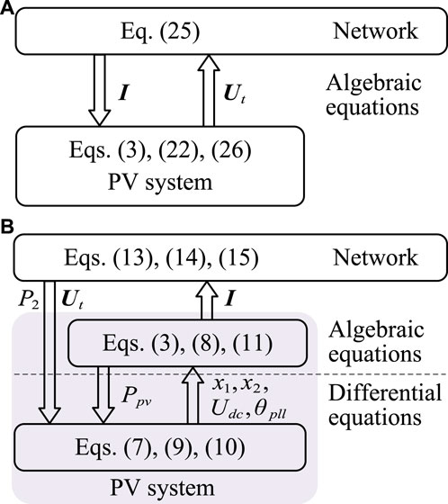
FIGURE 5. Input-output relationships between the PV system and the network within (A) the electromechanical timescale and (B) the electromagnetic timescale.

3.3 Fast subsystem

Similarly, taking τ = t/ɛ in (20) and performing the timescale transformation, the equivalent singular perturbation system can be obtained. Then, we have the differential equations of the fast subsystem:

$\left\{\begin{array}{c}{\tau }_1{\dot{x}}_1=U_{dc}-U_{\mathit{dcref}}\hfill \\ {\tau }_2{\dot{x}}_2=U_t-U_{\mathit{tref}}\hfill \\ {\tau }_3{\dot{x}}_3=\sin \left({\theta }_t-{\theta }_{\mathit{pll}}\right)\hfill \\ {\tau }_{\mathit{pll}}{\dot{\theta }}_{\mathit{pll}}=\sin \left({\theta }_t-{\theta }_{\mathit{pll}}\right)+x_3\hfill \\ {\tau }_C{\dot{U}}_{dc}=P_{pv}-P_2\hfill \end{array}\right.(27)$

Meanwhile, the differential equations for the slow variables (θ_g and ω_g) should be transformed into algebraic equations. Namely, θ_g = θ_g0 and ω_g = ω_g0, which are determined by the initial power flow of the full system. Consequently, the SG is equivalent to a constant voltage source, while the output of the PV system still functions as a controlled current source. The dynamics of the fast subsystem are dominated by the DVC, TVC, and PLL of the PV system within the electromagnetic timescale. Hence, the voltage vectors U_c and U_t, and electromagnetic active power P₁ and P₂, are the same as in (12), (13), (14) and (15), except that the slow variable θ_g is taken as θ_g0. At this point, the input-output relationship between the PV system and the network is illustrated in Figure 5B.

4 Transient synchronization stability analysis of the PV-SG system

4.1 Stability analysis of the slow subsystem

According to Eq. (21), the differential equations of the slow subsystem can be unified as

$M{\ddot{\theta }}_g+D{\dot{\theta }}_g+P\left({\theta }_g\right)=0(28)$

where M = T_j/ω₀, D = D₀/ω₀, P (θ_g) = P₁ − P_m, and P₁ denotes the output active power of the SG after the fault.

Then, the energy function can be constructed (Chiang, 2011):

$V\left({\theta }_g,{\dot{\theta }}_g\right)=\frac{1}{2}M{\left[{\dot{\theta }}_g\left(t\right)\right]}^2+{\int }_{{\theta }_g\left(t_0\right)}^{{\theta }_g\left(t\right)}P\left(\theta \right)d\theta (29)$

as

$\frac{dV}{dt}=\frac{\partial V}{\partial {\dot{\theta }}_g}\frac{d{\dot{\theta }}_g}{dt}+\frac{\partial V}{\partial {\theta }_g}\frac{d{\theta }_g}{dt}=-D{\left(\frac{d{\theta }_g}{dt}\right)}^2<0(30)$

In addition, the critical energy V_cr is the energy at the unstable equilibrium point θ_gu after the fault;

$V_{cr}=\frac{1}{2}M{\left[{\dot{\theta }}_{gu}\right]}^2+{\int }_{{\theta }_{gs}}^{{\theta }_{gu}}P\left(\theta \right)d\theta (31)$

The stable equilibrium point θ_gs and the unstable equilibrium point θ_gu can be obtained by solving the differential algebraic equations of the slow subsystem after the fault.

The θ_g0 denotes the stable equilibrium point of the slow subsystem before the fault. By comparing the energy V₀ at θ_g0 before the fault and the critical energy V_cr, the stability of the slow subsystem can be judged. The stability condition of the slow subsystem is V₀ < V_cr, namely,

${\int }_{{\theta }_{g0}}^{{\theta }_{gu}}P\left(\theta \right)d\theta >0(32)$

Clearly the stability of the slow subsystem primarily relies on the operating parameters P_m and P_pv, as well as the structural parameters X_g, X₁, and X₂, while it is unaffected by the control parameters and DC capacitance of the PV system.

According to the stability condition Eq. (32), for example, for a grid voltage dip fault, the critical grid voltage and grid reactances for a stable subsystem can be obtained. The result is illustrated in Figure 6A, where it is evident that larger U_g is beneficial for the system stability. The stable regions of the slow subsystem under different levels of PV penetration are shown in Figure 6B. The output active power P_pv of the PV system corresponds to 0.8 pu, 0.9 pu, and 1.0 pu, respectively. As illustrated, the range of the stable region diminishes with increasing P_pv. Therefore, a smaller P_pv improves the system stability. The impact of the equivalent line reactance X₂ is also investigated and the result is shown in Figure 6C. The reactance X₂ corresponds to 0.1 pu, 0.3 pu, and 0.5 pu, respectively. As observed, the stable region of the slow subsystem reduces with increasing X₂. Thus, a smaller X₂ is beneficial for the system stability.

FIGURE 6

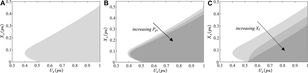
FIGURE 6. Stable regions of the slow subsystem based on the energy function analysis under (A) P_pv = 0.9 pu and X₂ = 0.1 pu, (B) increasing P_pv = 0.8, 0.9, and 1.0 pu, and (C) increasing X₂ = 0.1, 0.3, and 0.5 pu.

4.2 Stability analysis of the fast subsystem

The fast subsystem is regarded as a small disturbance of the slow subsystem, and the stability analysis can be carried out by linearization analysis methods (Kokotović et al., 1999; Ma et al., 2022b). By linearizing the fast subsystem on the operation point, the Jacobian matrix A of the fast subsystem can be obtained, as shown in Supplementary Material S2. If all the real parts of the eigenvalues of A are negative, the fast subsystem is asymptotically stable (Kundur, 1994). Based on A, it can be observed that the stability of the fast subsystem is affected by the control parameters of the DVC, TVC, and PLL, the steady-state operating parameters, and the structural parameters. Similarly, according to this stability condition of the fast subsystem, the stable region for different grid voltage U_g and grid reactance X_g under the grid voltage dips is illustrated in the purple region in Figure 7. In addition, the participation factor analysis is conducted. It is found that the state variables x₁, x₃, θ_pll, and U_dc show significant participation in the conjugate eigenvalues near the imaginary axis. Consequently, the stability of the fast subsystem is primarily affected by the DVC, PLL, and the dynamics of the DC capacitor, while the impact of the TVC is relatively slight.

FIGURE 7

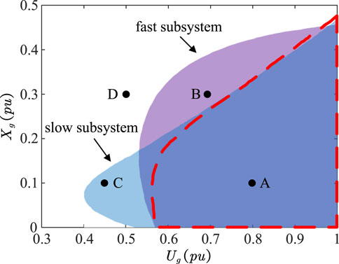
FIGURE 7. Comparison of stable regions under grid voltage dips. The bule region is the stable region of the slow subsystem based on the energy function analysis and the purple region is the stable region of the fast subsystem based on the eigenvalue analysis. Their intersection is the predicted stable region of the full system for both the slow and fast stable subsystems, while the region bounded by the red dashed line is the stable region of the full system based on the EMT simulations.

Next let us study the parameter impacts. With increasing the proportional coefficient K_p1 and integral coefficient K_i1 of the DVC, the eigenvalue loci of the fast subsystem are illustrated in Figures 8A,B, respectively. As K_p1 increases, the conjugate eigenvalues λ₁ and λ₂ gradually approach the imaginary axis from the right-half plane to the left-half one. The system stability is enhanced. Conversely, with the increase of K_i1, the conjugate eigenvalues λ₁ and λ₂ gradually move towards the imaginary axis from the left-half plane to the right-half one, and the system becomes unstable. Therefore, the larger K_p1 and smaller K_i1 of the DVC improve the stability of the fast subsystem.

FIGURE 8

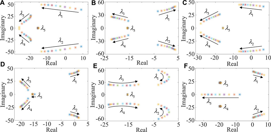
FIGURE 8. Eigenvalue loci with increasing control parameters of the DVC and PLL, and structural parameters: (A) K_p1, (B) K_i1, (C) K_p3, (D) K_i3, (E) C_dc, and (F) X₂.

As K_p3 and K_i3 of the PLL increase, the eigenvalue loci are shown in Figures 8C,D, respectively. It can be found that the larger K_p3 and smaller K_i3 of the PLL enhance the stability of the fast subsystem.

The eigenvalue loci with increasing the DC capacitance are illustrated in Figure 8E. As C_dc increases, the conjugate eigenvalues λ₁ and λ₂ gradually approach the imaginary axis from the left-half plane to the right-half one. Subsequently, they cross the imaginary axis again and move back towards the left-half plane. Therefore, as C_dc increases, the stability of the fast subsystem is initially weakened and subsequently improved.

In addition, the eigenvalue loci with increasing the equivalent line reactance X₂ are shown in Figure 8F. As X₂ increases, the conjugate eigenvalues λ₁ and λ₂ shift from the left-half plane to the right-half one, thereby deteriorating the stability of the fast subsystem. Consequently, a smaller X₂ improves the stability of the fast subsystem.

5 Simulation verification

5.1 Verification of the reduced-order model

In order to verify the validity of the fast and slow subsystem models, the time-domain simulation is conducted under the grid voltage dips. For the PV-SG parallel system in Figure 2, as a test, the system has reached a steady state before t = 1 s. At t = 1 s, again the grid voltage U_g suddenly dips from 1.0 pu to 0.8 pu, and the time domain responses of the rotor angle θ_g of the SG and the PLL output angle θ_pll are shown in Figure 9. The blue solid line represents the results of the full model, while the red dashed line and the purple dash-dotted line represent those of the slow and fast subsystem models, respectively.

FIGURE 9

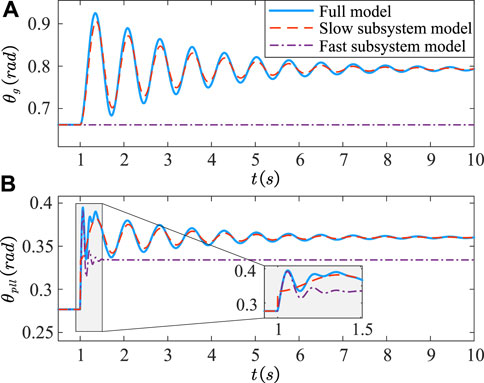
FIGURE 9. Time-domain simulation results of (A) the rotor angle θ_g and (B) the PLL output angle θ_pll of the full model (solid line), the slow subsystem model (dashed line), and the fast subsystem model (dash-dotted line) when the grid voltage U_g dips from 1.0 pu to 0.8 pu at t = 1 s under X_g = 0.1 pu.

In Figure 9A, the rotor angle θ_g oscillates and ultimately converges within the electromechanical timescale. The oscillation of the PLL output angle θ_pll within the electromagnetic timescale attenuates rapidly in the early stage after the fault [for the zoom-in plot in Figure 9B] and it shows electromechanical timescale dynamics in a long term. The response trajectories of the slow subsystem model essentially coincide with those of the full system. Additionally, the fast subsystem model captures the dynamics of the PLL output angle θ_pll in the early stage after the fault within the electromagnetic timescale. Therefore, the slow and fast subsystem models can truly reflect the dynamical behaviors of the full system during different transient processes, thereby verifying the validity and efficiency of the proposed model.

5.2 Verification of the stable regions

When both the slow and fast subsystems are stable, the full system is stable. Thus, the stable region of the full system corresponds to the intersection of the stable regions of the fast and slow subsystems, as illustrated by purple and blue, respectively, in Figure 7. The region bounded by the red dashed line represents the stable region of the full system obtained directly from the EMT simulations, which is essentially consistent with the analyses. Therefore, it is reasonable to catch the stability of the full system by performing the stability analysis of its fast and slow subsystems.

5.3 Verification of the stability analysis

So far, we have studied the case that both the fast and slow subsystems are stable, and hence the full system is stable in Figure 9, which corresponds to point A in Figure 7. Next let us study several other cases represented by points B, C, and D in Figure 7.

At t = 1 s, the grid voltage U_g dips from 1.0 pu to 0.7 pu under X_g = 0.3 pu, corresponding to point B in Figure 7. The time domain responses of the rotor angle θ_g and the PLL output angle θ_pll of the full system as well as the fast and slow subsystems are illustrated in Figure 10. The fast subsystem is stable while the slow subsystem is unstable, resulting in the instability of the full system. At this point, the response trajectories of the slow subsystem are roughly consistent with the full system.

FIGURE 10

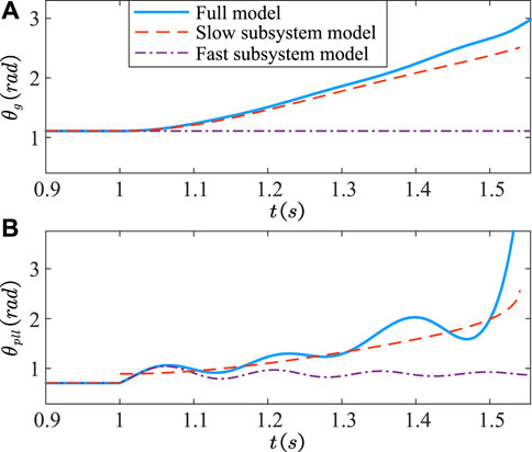
FIGURE 10. Time-domain simulation results of (A) the rotor angle θ_g and (B) the PLL output angle θ_pll. Similar to Figure 9, but for U_g dips to 0.7 pu under X_g = 0.3 pu, instead. Now the fast subsystem is stable, but the slow subsystem is unstable.

The grid voltage U_g dips to 0.45 pu under X_g = 0.1 pu, corresponding to point C in Figure 7. The time domain responses of θ_g and θ_pll of the full system as well as the fast and slow subsystems are illustrated in Figure 11. Now the slow subsystem is stable while the fast subsystem is unstable, and the full system is unstable.

FIGURE 11

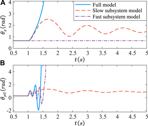
FIGURE 11. Time-domain simulation results of (A) the rotor angle θ_g and (B) the PLL output angle θ_pll. Similar to Figure 9, but for U_g dips to 0.45 pu under X_g = 0.1 pu, instead. Now the slow subsystem is stable, while the fast subsystem is unstable.

The grid voltage U_g dips to 0.5 pu under X_g = 0.3 pu, corresponding to point D in Figure 7. The time domain responses of θ_g and θ_pll of the full system as well as the fast and slow subsystems are illustrated in Figure 12. Here both the fast and slow subsystems are unstable, and the full system is unstable.

FIGURE 12

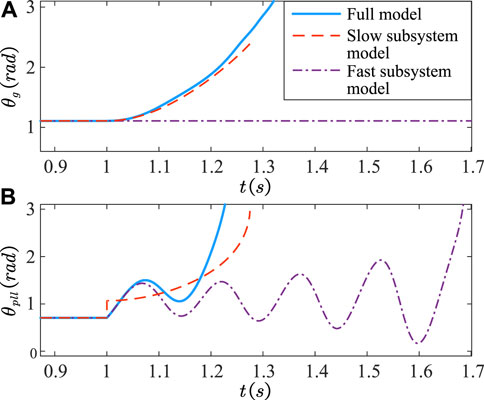
FIGURE 12. Time-domain simulation results of (A) the rotor angle θ_g and (B) the PLL output angle θ_pll. Similar to Figure 9, but for U_g dips to 0.5 pu under X_g = 0.3 pu, instead. Now both the fast and slow subsystems are unstable.

Therefore, the above simulation results perfectly verify that the full system is stable when both the fast and slow subsystems are stable. Moreover, when the fast subsystem is stable, the slow subsystem can reflect the dynamical behaviors of the full system in a long time perspective.

5.4 Verification of the parameter impacts

To verify the impacts of different parameters obtained from the theoretical analysis, broad EMT simulations have been conducted. For example, in Case 1, the parameters are set as follows: k_p1 = 3.5, k_i1 = 140, k_p3 = 50, k_i3 = 2000, C_dc = 0.1 pu. We can change one parameter each time in different Cases: e.g., k_p1 = 7 (Case 2); k_i1 = 60 (Case 3); k_p3 = 100 (Case 4); k_i3 = 200 (Case 5); C_dc = 0.01 pu (Case 6); C_dc = 0.5 pu (Case 7). At t = 1 s, the voltage U_g suddenly dips from 1.0 pu to 0.5 pu. Figure 13 shows the time domain responses of the rotor angle θ_g and the PLL output angle θ_pll under these Cases. As illustrated, the system remains stable under all these Cases, except for Case 1. Therefore, larger K_p1 and K_p3, and smaller K_i1 and K_i3 can enhance the system stability. The system stability is initially weakened and then improved with an increase of C_dc. In addition, the impacts of levels of PV penetration and equivalent line reactances are also investigated. At t = 1 s, the grid voltage U_g dips from 1.0 pu to 0.65 pu. The corresponding responses of the rotor angle θ_g under different levels of PV penetration and equivalent line reactances are illustrated in Figures 14A,B, respectively. It is evident that smaller P_pv and X₂ improve the system stability. All these simulation results are consistent with the findings of the previous theoretical analysis.

FIGURE 13

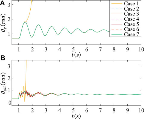
FIGURE 13. Time-domain simulation results of (A) the rotor angle θ_g and (B) the PLL output angle θ_pll. Transient responses of the rotor angle θ_g and the PLL output angle θ_pll under different Cases when the grid voltage U_g dips from 1.0 pu to 0.5 pu at t = 1 s.

FIGURE 14

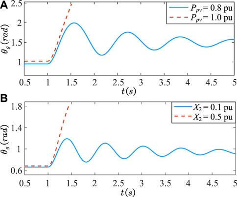
FIGURE 14. Transient responses of the rotor angle θ_g when the grid voltage U_g dips from 1.0 pu to 0.65 pu at t =1 s under different levels of PV penetration and equivalent line reactances. (A) P_pv = 0.8 pu and 1.0 pu under X_g = 0.2 pu. (B) X₂ = 0.1 pu and 0.5 pu under X_g = 0.1 pu.

6 Conclusion and discussion

In conclusion, the transient synchronization stability of the PV-SG system is studied by using the singular perturbation technique. Compared to the most existing research endeavors on the wide simulations of the PVs integration, the impact of PVs on the synchronization dynamics of SGs without considering the dynamical characteristics of the PV system, and the transient synchronization stability analyses of the PLL-based VSC systems, this paper provides a clearer physical picture for the dynamical characteristics of the PV system and deeply studies its interaction with the SG under different timescales. The main conclusions are summarized as follows:

1) The dynamical behaviors of the PV-SG system show multi-timescale characteristics during the transient processes. The proposed reduced-order fast-slow subsystem model can effectively reflect the dynamical behaviors of the full system within the electromagnetic and electromechanical timescales. Moreover, when the fast subsystem is stable, the slow subsystem can describe the transient process of the full system, especially in a long time perspective.

2) Based on the slow and fast subsystems, the stability of the full PV-SG system is analyzed using the energy function and eigenvalue analysis methods. In addition, the full system is stable only when both the fast and slow subsystems are stable.

3) Lower levels of PV penetration, smaller equivalent line reactance, larger proportional coefficients, and smaller integral coefficients of the DVC and PLL enhance the system stability. Furthermore, as the DC capacitance increases, the system stability is initially weakened and then improved.

For discussions, it is necessary to give some important points:

1) The transient characteristics of the PV-SG system remain essentially unchanged when considering the damper and excitation windings of the SG. The dynamics of the damper and excitation windings belong to the ACC and electromechanical timescales, respectively, and the rotor angle is still dominated by the electromechanical timescale dynamics. The dominant dynamical behaviors of the PLL output angle is slightly affected by the damper and excitation windings of the SG in the early stage after the fault. Consequently, it is reasonable and effective to use the classical second-order model of the SG for studying the transient synchronization stability of the PV-SG system.

2) For the transient synchronization stability of the PV-SG system, it is difficult to directly use the energy function method in the full high-order PV-SG system. In this paper, the full seventh-order PV-SG system is decomposed into a second-order slow subsystem and a fifth-order fast subsystem by using the singular perturbation technique. Further, the transient synchronization stability of the PV-SG system is investigated using the energy function and eigenvalue analysis methods. Compared to the most existing methods, this paper provides a clearer physical picture for the dynamical characteristics of the PV system and deeply studies its interaction with the SG under different timescales. In addition, we utilize a PV-SG parallel system to study the transient synchronization stability of PVs integration in this paper. The reduced-order modeling method in this paper is also applicable to multi-machine power systems integrated with PVs, and some work has been done in our recent research (Wu et al., 2023). The transient synchronization stability of the full system can also be studied based on the slow and fast subsystems. However, due to the high-order and strong coupling of multi-machine systems, it is still very challenging to perform the transient synchronization stability analysis of multi-machine systems, which needs further consideration in our future work.

3) For the impacts of different PV penetration levels, it is found that lower levels enhance the transient synchronization stability of the PV-SG system in this paper. However, this conclusion is derived from the simple PV-SG parallel system and cannot be directly extended to a more generalized PV-SG system. Due to various influencing factors, a unified perspective on whether lower PV penetration levels enhance transient synchronization stability still lacks, which needs further investigation. Nevertheless, the reduced-order modeling and stability analysis methods, based the slow and fast subsystems, are equally applicable to a more generalized PV-SG system. The impacts of different PV penetration levels on the system stability can be analyzed similarly from the perspective of corresponding subsystems.

4) While many studies focus on the second-order PLL for the transient synchronization stability of the PLL-based VSC system, they assume the outputs from outer DVC and TVC (i.e., the current references) are constant, which is only valid for certain situations, such as the low voltage ride through. The current references of the PV-SG system change during the transient processes. Thus, it is inappropriate to only consider the PLL and neglect the DVC in the modeling and analysis of the PV-SG system for generalized situations. In (Ma et al., 2023d), it is uncovered that not only the PLL but also the DVC plays an important role in transient dynamics. Moreover, in this paper, it is found that the DVC affects the stability of the fast subsystem and may lead further instability in the full system. For the DVC parameters, they only influence the stability of the fast subsystem, with no effect on the stability of the slow subsystem. It is revealed that a larger proportional coefficient and a smaller integral coefficient of the DVC enhance the stability of the fast subsystem. Consequently, when the fast subsystem becomes unstable after a fault due to improper DVC parameters, the full system also becomes unstable. When the fast subsystem remains stable after a fault, the dominant dynamical behaviors of the full system are unaffected by DVC parameters, as the full system is then dominated by the slow subsystem dynamics. In this paper, the fifth-order fast subsystem is treated as a small disturbance of the slow subsystem and analyzed by the linearization analysis method. For the transient synchronization stability of the PV-SG system, the effective nonlinear analysis methods still lack, which should be further studied.

Data availability statement

The original contributions presented in the study are included in the article/Supplementary Material, further inquiries can be directed to the corresponding author.

Author contributions

JW: Conceptualization, Formal Analysis, Methodology, Software, Writing–original draft, Writing–review and editing. MH: Data curation, Formal Analysis, Software, Writing–original draft. MZ: Conceptualization, Funding acquisition, Investigation, Resources, Supervision, Writing–review and editing.

Funding

The author(s) declare financial support was received for the research, authorship, and/or publication of this article. This work was supported by the National Natural Science Foundation of China, grant numbers 12075091 and U22B6008.

Conflict of interest

The authors declare that the research was conducted in the absence of any commercial or financial relationships that could be construed as a potential conflict of interest.

Publisher’s note

All claims expressed in this article are solely those of the authors and do not necessarily represent those of their affiliated organizations, or those of the publisher, the editors and the reviewers. Any product that may be evaluated in this article, or claim that may be made by its manufacturer, is not guaranteed or endorsed by the publisher.

Supplementary material

The Supplementary Material for this article can be found online at: https://www.frontiersin.org/articles/10.3389/fenrg.2024.1332272/full#supplementary-material

References

Chen, T., Feng, D., Wu, X., Lu, C., and Xu, B. (2023). Modeling and stability analysis of interaction between converters in ac-dc distribution systems. Front. Energy Res. 10. doi:10.3389/fenrg.2022.1035193

CrossRef Full Text | Google Scholar

Chiang, H.-D. (2011). Direct methods for stability analysis of electric power systems: theoretical foundation, BCU methodologies, and applications. Hoboken, NJ, USA: Wiley.

Google Scholar

Eftekharnejad, S., Vittal, V., Heydt, G. T., Keel, B., and Loehr, J. (2013). Impact of increased penetration of photovoltaic generation on power systems. IEEE Trans. Power Syst. 28, 893–901. doi:10.1109/TPWRS.2012.2216294

CrossRef Full Text | Google Scholar

Fu, X., Huang, M., Pan, S., and Zha, X. (2022). Cascading synchronization instability in multi-vsc grid-connected system. IEEE Trans. Power Electron. 37, 7572–7576. doi:10.1109/TPEL.2022.3153283

CrossRef Full Text | Google Scholar

Gandhi, O., Kumar, D. S., Rodríguez-Gallegos, C. D., and Srinivasan, D. (2020). Review of power system impacts at high PV penetration part I: factors limiting PV penetration. Sol. Energy 210, 181–201. doi:10.1016/j.solener.2020.06.097

CrossRef Full Text | Google Scholar

He, C., He, X., Geng, H., Sun, H., and Xu, S. (2022a). Transient stability of low-inertia power systems with inverter-based generation. IEEE Trans. Energy Convers. 37, 2903–2912. doi:10.1109/TEC.2022.3185623

CrossRef Full Text | Google Scholar

He, H., Xia, Y., Wei, W., and Yang, P. (2022b). Transient stability analysis and control of distributed photovoltaic generators in the dc distribution network. Front. Energy Res. 10. doi:10.3389/fenrg.2022.875654

CrossRef Full Text | Google Scholar

He, X., and Geng, H. (2021). Transient stability of power systems integrated with inverter-based generation. IEEE Trans. Power Syst. 36, 553–556. doi:10.1109/TPWRS.2020.3033468

CrossRef Full Text | Google Scholar

He, X., and Geng, H. (2022). Pll synchronization stability of grid-connected multiconverter systems. IEEE Trans. Industry Appl. 58, 830–842. doi:10.1109/TIA.2021.3121262

CrossRef Full Text | Google Scholar

Hossain, M. K., and Ali, M. H. (2015). Transient stability augmentation of pv/dfig/sg-based hybrid power system by nonlinear control-based variable resistive fcl. IEEE Trans. Sustain. Energy 6, 1638–1649. doi:10.1109/TSTE.2015.2463286

CrossRef Full Text | Google Scholar

Kabeyi, M. J. B., and Olanrewaju, O. A. (2022). Sustainable energy transition for renewable and low carbon grid electricity generation and supply. Front. Energy Res. 9, 743114. doi:10.3389/fenrg.2021.743114

CrossRef Full Text | Google Scholar

Khalil, H. K. (2002). Nonlinear systems. 3rd edn. Upper Saddle River, N.J: Prentice Hall.

Google Scholar

Kokotović, P., Khalil, H. K., and O’reilly, J. (1999). Singular perturbation methods in control: analysis and design. Unites States: SIAM.

Google Scholar

Kumar, D. S., Sharma, A., Srinivasan, D., and Reindl, T. (2019). Stability implications of bulk power networks with large scale PVs. Energy 187, 115927. doi:10.1016/j.energy.2019.115927

CrossRef Full Text | Google Scholar

Kundur, P. (1994). Power system stability and control. New York, NY, USA: McGraw-Hill.

Google Scholar

Landera, Y. G., Zevallos, O. C., Neves, F. A. S., Neto, R. C., and Prada, R. B. (2022). Control of pv systems for multimachine power system stability improvement. IEEE Access 10, 45061–45072. doi:10.1109/ACCESS.2022.3169791

CrossRef Full Text | Google Scholar

Li, X., Tian, Z., Zha, X., Sun, P., Hu, Y., Huang, M., et al. (2023). Nonlinear modeling and stability analysis of grid-tied paralleled-converters systems based on the proposed dual-iterative equal area criterion. IEEE Trans. Power Electron. 38, 7746–7759. doi:10.1109/TPEL.2023.3246763

CrossRef Full Text | Google Scholar

Liu, D., Chen, S., Ma, M., Wang, H., Hou, J., and Ma, S. (2011). A review on models for photovoltaic generation system. Power Syst. Technol. 35, 47–52. doi:10.13335/j.1000-3673.pst.2011.08.017

CrossRef Full Text | Google Scholar

Ma, R., Yang, Z., Cheng, S., and Zhan, M. (2020). Sustained oscillations and bifurcations in three-phase voltage source converter tied to AC grid. IET Renew. Power Gener. 14, 3770–3781. doi:10.1049/iet-rpg.2020.0204

CrossRef Full Text | Google Scholar

Ma, R., Li, J., Kurths, J., Cheng, S., and Zhan, M. (2022a). Generalized swing equation and transient synchronous stability with PLL-based VSC. IEEE Trans. Energy Convers. 37, 1428–1441. doi:10.1109/TEC.2021.3137806

CrossRef Full Text | Google Scholar

Ma, Y., Zhu, D., Zhang, Z., Zou, X., Hu, J., and Kang, Y. (2022b). Modeling and transient stability analysis for type-3 wind turbines using singular perturbation and Lyapunov methods. IEEE Trans. Industrial Electron. 70, 8075–8086. doi:10.1109/TIE.2022.3210484

CrossRef Full Text | Google Scholar

Ma, R., Zhan, M., Jiang, K., Liu, D., Hu, P., and Cheng, S. (2023a). Transient stability assessment of renewable dominated power systems by the method of hyperplanes. IEEE Trans. Power Deliv. 38, 3455–3468. doi:10.1109/TPWRD.2023.3281814

CrossRef Full Text | Google Scholar

Ma, R., Zhang, Y., Han, M., Kurths, J., and Zhan, M. (2023b). Synchronization stability and multi-timescale analysis of renewable-dominated power systems. Chaos 33, 082101. doi:10.1063/5.0156459

PubMed Abstract | CrossRef Full Text | Google Scholar

Ma, R., Zhang, Y., Yang, Z., Kurths, J., Zhan, M., and Lin, C. (2023c). Synchronization stability of power-grid-tied converters. Chaos 33, 032102. doi:10.1063/5.0136975

PubMed Abstract | CrossRef Full Text | Google Scholar

Ma, R., Zhang, Y., Zhan, M., Cao, K., Liu, D., Jiang, K., et al. (2023d). Dominant transient equations of grid-following and grid-forming converters by controlling-unstable-equilibrium-point-based participation factor analysis. IEEE Trans. Power Syst. 99, 1–17. doi:10.1109/TPWRS.2023.3332882

CrossRef Full Text | Google Scholar

NERC Joint and WECC Staff (2018). “900 MW solar photovoltaic resource interruption disturbance report,”. Tech. Rep. (Atlanta, GA, USA: NERC).

Google Scholar

Pico, H. N. V., and Johnson, B. B. (2019). Transient stability assessment of multi-machine multi-converter power systems. IEEE Trans. Power Syst. 34, 3504–3514. doi:10.1109/TPWRS.2019.2898182

CrossRef Full Text | Google Scholar

Priyamvada, I. R. S., and Das, S. (2020a). Online assessment of transient stability of grid connected pv generator with dc link voltage and reactive power control. IEEE Access 8, 220606–220619. doi:10.1109/ACCESS.2020.3042784

CrossRef Full Text | Google Scholar

Priyamvada, I. R. S., and Das, S. (2020b). Transient stability of V_dc– Q control-based PV generator with voltage support connected to grid modelled as synchronous machine. IEEE Access 8, 130354–130366. doi:10.1109/ACCESS.2020.3008942

CrossRef Full Text | Google Scholar

Rezaei, J., Golshan, M. E. H., and Alhelou, H. H. (2022). Impacts of integration of very large-scale photovoltaic power plants on rotor angle and frequency stability of power system. IET Renew. Power Gener. 16, 2384–2401. doi:10.1049/rpg2.12529

CrossRef Full Text | Google Scholar

Seane, T., Samikannu, R., and Bader, T. (2022). A review of modeling and simulation tools for microgrids based on solar photovoltaics. Front. Energy Res. 10, 772561. doi:10.3389/fenrg.2022.772561

CrossRef Full Text | Google Scholar

Shah, R., Mithulananthan, N., Bansal, R., and Ramachandaramurthy, V. (2015). A review of key power system stability challenges for large-scale PV integration. Renew. Sustain. Energy Rev. 41, 1423–1436. doi:10.1016/j.rser.2014.09.027

CrossRef Full Text | Google Scholar

Shchepakina, E., Mortell, M. P., and Sobolev, V. (2014). Singular perturbations: introduction to system order reduction methods with applications. Berlin, Germany: Springer.

Google Scholar

Shen, C., Shuai, Z., Shen, Y., Peng, Y., Liu, X., Li, Z., et al. (2021). Transient stability and current injection design of paralleled current-controlled vscs and virtual synchronous generators. IEEE Trans. Smart Grid 12, 1118–1134. doi:10.1109/TSG.2020.3032610

CrossRef Full Text | Google Scholar

Tamimi, B., Cañizares, C., and Bhattacharya, K. (2013). System stability impact of large-scale and distributed solar photovoltaic generation: the case of ontario, Canada. IEEE Trans. Sustain. Energy 4, 680–688. doi:10.1109/TSTE.2012.2235151

CrossRef Full Text | Google Scholar

Villalva, M., Gazoli, J., and Filho, E. (2009). Comprehensive approach to modeling and simulation of photovoltaic arrays. IEEE Trans. Power Electron. 24, 1198–1208. doi:10.1109/TPEL.2009.2013862

CrossRef Full Text | Google Scholar

Wang, X., Taul, M. G., Wu, H., Liao, Y., Blaabjerg, F., and Harnefors, L. (2020). Grid-synchronization stability of converter-based resources—an overview. IEEE Open J. Industry Appl. 1, 115–134. doi:10.1109/OJIA.2020.3020392

CrossRef Full Text | Google Scholar

Wu, H., and Wang, X. (2020). Design-oriented transient stability analysis of PLL-synchronized voltage-source converters. IEEE Trans. Power Electron. 35, 3573–3589. doi:10.1109/TPEL.2019.2937942

CrossRef Full Text | Google Scholar

Wu, J., Han, M., and Zhan, M. (2023). “Nonlinear multiscale modeling of multi-machine power systems integrated with photovoltaics,” in 2023 IEEE PELS Students and Young Professionals Symposium (SYPS), Shanghai, China, 27-29 August 2023, 1–6. doi:10.1109/SYPS59767.2023.10268127

CrossRef Full Text | Google Scholar

Xiong, L., Liu, X., Liu, Y., and Zhuo, F. (2022). Modeling and stability issues of voltage-source converter-dominated power systems: a review. CSEE J. Power Energy Syst. 8, 1530–1549. doi:10.17775/CSEEJPES.2020.03590

CrossRef Full Text | Google Scholar

Xu, Z., Qin, Y., Li, Z., Jiao, C., Zhai, B., and Chang, X. (2023). Stability analysis of different control modes of grid-connected converters under different grid conditions. Front. Energy Res. 11, 1242024. doi:10.3389/fenrg.2023.1242024

CrossRef Full Text | Google Scholar

Yang, Z., Ma, R., Cheng, S., and Zhan, M. (2020). Nonlinear modeling and analysis of grid-connected voltage-source converters under voltage dips. IEEE J. Emerg. Sel. Top. Power Electron. 8, 3281–3292. doi:10.1109/JESTPE.2020.2965721

CrossRef Full Text | Google Scholar

Yuan, X., Hu, J., and Cheng, S. (2017). Multi-time scale dynamics in power electronics-dominated power systems. Front. Mech. Eng. 12, 303–311. doi:10.1007/s11465-017-0428-z

CrossRef Full Text | Google Scholar

Zevallos, O. C., Silva, J. B. D., Mancilla-David, F., Neves, F. A. S., Neto, R. C., and Prada, R. B. (2021). Control of photovoltaic inverters for transient and voltage stability enhancement. IEEE Access 9, 44363–44373. doi:10.1109/ACCESS.2021.3066147

CrossRef Full Text | Google Scholar

Zhang, C., Molinas, M., Li, Z., and Cai, X. (2020). Synchronizing stability analysis and region of attraction estimation of grid-feeding vscs using sum-of-squares programming. Front. Energy Res. 8, 56. doi:10.3389/fenrg.2020.00056

CrossRef Full Text | Google Scholar

Zhang, Y., Han, M., and Zhan, M. (2023). The concept and understanding of synchronous stability in power electronic-based power systems. Energies 16, 2923. doi:10.3390/en16062923

CrossRef Full Text | Google Scholar

Zhang, Y., Zhang, C., and Cai, X. (2022). Large-signal grid-synchronization stability analysis of PLL-based VSCs using Lyapunov’s direct method. IEEE Trans. Power Syst. 37, 788–791. doi:10.1109/TPWRS.2021.3089025

CrossRef Full Text | Google Scholar

Zhao, J., Huang, M., Yan, H., Tse, C. K., and Zha, X. (2021). Nonlinear and transient stability analysis of phase-locked loops in grid-connected converters. IEEE Trans. Power Electron. 36, 1018–1029. doi:10.1109/TPEL.2020.3000516

CrossRef Full Text | Google Scholar