A novel recognition method for complex power quality disturbances based on Markov transition field and improved densely connected network

In order to solve the difficulty that complex power quality disturbances (PQDs) are difficult to recognize accurately and efficiently under the new power system background, this paper proposes a novel PQDs recognition method based on markov transition field (MTF) and improved densely connected network (DenseNet). Firstly, the one-dimensional PQDs signal is mapped into the two-dimensional image with clear texture features by using MTF encoding method. Then, a DenseNet-S lightweight network is designed and the convolutional attention module (CBAM) is introduced to improve its feature extraction ability, so as to enhance the performance of the network. Finally, the images are input into the improved model for training and learning, and PQDs recognition is realized through the optimal model. In order to verify the effectiveness of the proposed method, experimental tests are carried out based on IEEE 1159 standard simulation dataset and real-world field measured signals dataset, and compared with existing recognition methods. The results show that the proposed method can effectively improve the recognition accuracy and noise robustness of complex PQDs, and has more advantages in disturbances recognition efficiency. It can meet the recognition accuracy and efficiency requirements of massive and complex PQDs events in engineering applications.

1 Introduction

With the increase of the penetration rate of distributed source loads, which is mainly dominated by wind and solar power generation and new energy charging piles, the power system presents a typical trend of power electronization (Wang et al., 2021), and the PQDs problem of power grid has shown some new features compared with the past. The typical features mainly include two points: 1) the expansion of the scale of new power system disturbance sources; 2) the coupling and superposition of PQDs are strengthened (Wang and Chen, 2019). The interactive coupling of PQDs will exhibit extremely complex non-stationary fluctuation phenomena and further deteriorate the grid power quality, which will not only bring problems such as sensitive equipment damage, data loss, equipment energy consumption increase and other problems to the end user side, but even lead to large-scale power outage accidents in serious cases (Cui et al., 2022). PQDs recognition algorithm is mainly used in the monitoring and management of power systems and power equipment, which can help us detect and identify power quality problems, such as voltage sag, harmonic, flicker, etc., which is crucial to ensure the stable operation of power system, prevent equipment damage and improve the electrical energy use efficiency. Therefore, accurate and efficient classification and recognition of PQDs under the new power system background is the basic requirement to ensure the safe, stable and economic operation of power grid.

The traditional PQDs recognition methods are based on manually extracting features, constructing feature matrices, and using the feature data to train classification model to realize disturbances recognition. Amongst these, feature extraction mostly applies signal processing techniques such as Fourier transform (Huang et al., 2016), Stockwell transform (Yin et al., 2021; Cui et al., 2022), and wavelet transform (Wu et al., 2022). After manual feature extraction, classification algorithms such as support vector machine (Tang et al., 2020), decision tree (Huang et al., 2017a), and artificial neural network (Li et al., 2020) are combined to establish the mapping relationship from continuous features to discrete labels to realize the classification and identification of PQDs. However, the parameter selection and processing process of the above methods are cumbersome, and heavily rely on expert experience, which makes it less generalizable. With the growing penetration of new energy sources, the complexity of PQDs increases accordingly, and the classification methods based on artificial feature extraction are difficult to meet the needs of PQDs classification under the new power system background.

In recent years, deep learning technology has become an important research hotspot in the field of PQDs recognition due to its excellent generalization performance and feature self-extraction capability. Among them, the deep learning methods that have been widely researched and applied are the Convolutional Neural Network (CNN), which can extract spatial features, and the Recurrent Neural Network (RNN), which has the memory ability of temporal features, to mine the potential relationship between spatial and temporal features of one-dimensional PQDs signals, and then recognize the specific type of PQDs (Ahmadi and Tani, 2019; Wang and Chen, 2019; Sindi et al., 2021). However, although the one-dimensional convolutional layer used in this method can extract temporal features to a certain extent, its temporal characteristics and disturbances classification ability are significantly reduced, and the problem of network gradient vanishing is serious. At the same time, it is not effective in dealing with the problem of feature extraction for multi-type coupling PQDs. To overcome the above problems, some scholars combine the advantages of machine vision and propose the visual conversion of one-dimensional signals, such as Gramian Angular Field (GAF), combined with the current mainstream image classification networks, such as CNN, deep residual network (ResNet), to discover the absolute temporal and spatial relationships of the original signal, and then extract more complete deep-level features of disturbance signals. He et al. (2023) and Jyoti et al. (2021) use the GAF color coding method to convert one-dimensional disturbance signals into rectangular images with different pattern features, which are used as inputs to CNN and ResNet for training and classification respectively, making up for the defects of artificial feature selection. However, GAF uses the Cartesian coordinate system to encode sequences in polar coordinates, and then converts them into Gram matrix using trigonometric operations, which is a complex cross-domain encoding conversion process, computationally intensive, and prone to aliasing with noise. At the same time, its conversion efficiency is on the low side, which makes it difficult to satisfy the recognition efficiency demand of massive and complex PQDs events in engineering practice.

Overall, there have been limited investigations into integrating signal visualization with image classification networks to recognize complex PQDs. Existing studies mainly concentrate on enhancing the disturbances recognition accuracy of the overall method, ignoring the performance of visualization imaging technology and deep learning model in terms of conversion and recognition efficiency. With the massive increase of power quality monitoring data, the recognition efficiency of PQDs is becoming increasingly crucial for power system health condition monitoring. To address this challenge, a novel PQDs recognition method based on MTF and improved DenseNet-SC is proposed in this paper. The proposed method utilizes the MTF encoding method with straightforward and efficient conversion process and clear features to color code the original disturbance signal to form PQDs feature image, and then designing lightweight network DenseNet-S and integrating CBAM attention mechanism to improve the feature capturing ability of the model. Finally, based on IEEE standard and the real-world field data collected by the substation, simulation and measurement dataset of PQDs are established to test the proposed method. The experimental results verify the effectiveness and superiority of the proposed method in PQDs recognition efficiency and precision.

2 PQDs data visualization based on MTF

2.1 PQDs model construction

For various complicated PQDs problems in power system, the real data is difficult to be collected by equipment. Therefore, according to IEEE Std, 2019 power quality standard, mathematical modeling of PQDs signal is carried out in this paper. The nine categories for common basic disturbance signals are sag, swell, interruption, harmonic, oscillatory transient, pulse, flicker, gap, and spike. Corresponding mathematical models for these categories are presented in Table 1.

TABLE 1

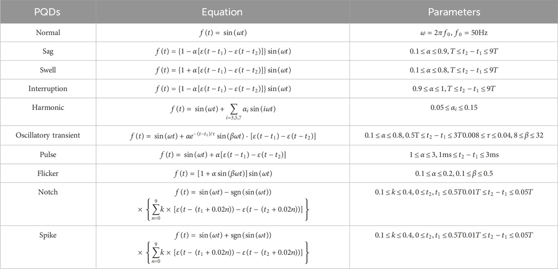
TABLE 1. Mathematical model of PQDs.

Complex PQDs are typically overlaid with multiple basic disturbances, including a variety of different categories and different start and end times. The resulting composite waveforms exhibit a complex, cumbersome, and irregular pattern, posing challenges in accurately recognizing the disturbance types.

2.2 Markov transition field

The conversion methods of one-dimensional PQD signal into two-dimensional image are currently mainly investigated using the GAF and its variants. However, due to the need for cross-domain encoding and matrix operation of sequence data, the conversion process of GAF is complex and low efficiency. In addition, the loss of time sequence feature information is easy to occur when processing disturbance signals in noisy environment.

To address the above shortcomings and deficiencies, this paper proposes a visual conversion method of PQDs based on MTF. The correlation between amplitude and time is the main relationship in time-series data. MTF can convert one-dimensional time series data into two-dimensional feature images by considering the time and position information on the basis of Markov chain and using Markov transition probability for coding, so as to maintain the time order and statistical dynamics in the generated images (Wang and Oates, 2015). Due to its excellent time-series information retention ability, MTF coding technology has been partially applied in fault diagnosis (Yan et al., 2022) and surface electromyography signal analysis (Li et al., 2022). However, as far as we know, MTF coding technology has not been applied to PQDs recognition research in the existing literature.

Given a set of time series signal $X=\left\{x_1,x_2,\dots ,x_N\right\}$, $x_i$ is the i-th sampling signal point. MTF method firstly divides the time series signal into $Q$ quantile units $q_j\left(j\in \left[1,Q\right]\right)$ according to its amplitude for discretization processing, quantizes each value, and any numerical point $x_i$ can be mapped to the corresponding quantile $q_i$. Then, by calculating the probability of sampling signal point $x_{t-1}$ and $x_t$ transferring from region $q_i$ to $q_j$ in the form of a first-order Markov chain along the time axis, and taking each calculated probability $p$ as element $w_{ij}$, the Markov state transition matrix $\mathit{W}$ of $Q\times Q$ dimension is constructed. The expression is shown in Eq. 1:

$\mathit{W}=\left[\begin{array}{cccc}{w}_{11}& w_{12}& \cdots & w_{1Q}\\ w_{21}& w_{22}& \cdots & w_{2Q}\\ ⋮& ⋮& \ddots & ⋮\\ w_{Q1}& w_{Q2}& \cdots & w_{QQ}\end{array}\right]=\left[\begin{array}{ccc}{p}_{1,1}\left(x_t\in q_1|x_{t-1}\in q_1\right)& \cdots & p_{1,Q}\left(x_t\in q_1|x_{t-1}\in q_Q\right)\\ p_{2,1}\left(x_t\in q_2|x_{t-1}\in q_1\right)& \cdots & p_{2,Q}\left(x_t\in q_2|x_{t-1}\in q_Q\right)\\ ⋮& \ddots & ⋮\\ p_{Q,1}\left(x_t\in q_Q|x_{t-1}\in q_1\right)& \cdots & p_{Q,Q}\left(x_t\in q_Q|x_{t-1}\in q_Q\right)\end{array}\right](1)$

Nonetheless, Markov chain is memoryless, and the probability of state transition at the current moment only depends on the state at the previous moment, without considering the dynamic probability transition of time series data. Therefore, the Markov state transition matrix constructed by Markov chain is also memoryless, which completely ignores the dependence of time step on one-dimensional time series signal $X$. If the Markov state transition matrix is used directly, a large amount of one-dimensional time series information will be lost. To solve this problem, MTF is used to improve it. By considering the time and position relationship, each transition probability is arranged in time order, and the Markov state transition matrix $\mathit{W}$ is extended to the MTF matrix $\mathit{M}$ across time scales, preserving the time correlation of the original signal. The expression of $\mathit{M}$ is shown in Eq. 2:

$\mathit{M}=\left[\begin{array}{cccc}{M}_{11}& M_{12}& \cdots & M_{1N}\\ M_{21}& M_{22}& \cdots & M_{2N}\\ ⋮& ⋮& \ddots & ⋮\\ M_{N1}& M_{N2}& \cdots & M_{NN}\end{array}\right]=\left[\begin{array}{ccc}{p}_{i,j}\left(x_1\in q_i|x_1\in q_j\right)& \cdots & p_{i,j}\left(x_1\in q_i|x_N\in q_j\right)\\ p_{i,j}\left(x_2\in q_i|x_1\in q_j\right)& \cdots & p_{i,j}\left(x_2\in q_i|x_N\in q_j\right)\\ ⋮& \ddots & ⋮\\ p_{i,j}\left(x_N\in q_i|x_1\in q_j\right)& \cdots & p_{i,j}\left(x_N\in q_i|x_N\in q_j\right)\end{array}\right](2)$

where $M_{mn}$ represents the probability of transferring from quantile region $q_i$ corresponding to sampling signal point $x_m$ to region $q_j$ corresponding to $x_n$, that is, the transition probability of the quantile relationship between $q_i$ and $q_j$ on the matrix $\mathit{W}$, while the elements on the diagonal are the corresponding self-transfer probability.

Taking one-dimensional sinusoidal signal as an instance, according to the above MTF dynamic transfer information encoding method, its two-dimensional MTF visual image generation process is shown in Figure 1.

FIGURE 1

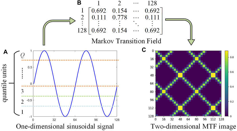
FIGURE 1. MTF visualization image generation process.

Considering that when $N$ is large, using the original MTF to directly generate images will make the images too large and occupy more computer storage space, which is not conducive to the rapid calculation and analysis of on-site intelligent devices or grid background systems. For this purpose, fuzzy kernel ${\left\{1/n^2\right\}}_{n\times n}$ is used to average each non-overlapping pixel to obtain a two-dimensional MTF image of the aggregated $n\times n$ dimension, that is, an aggregated image with dynamic transition probability, which is used as the image modal input data for power quality analysis.

The MTF image coding method offers a technique for visualizing sequences that maintains time dependency. The use of MTF to convert time series signals has the following advantages:

(1) By considering the dependence between each quantile unit and time step, the correlation between moments can be effectively represented, and the time series information loss of one-dimensional sequence signals can be avoided;

(2) The one-dimensional time-series signal and MTF image coding method are mapped relations, preventing the loss of feature information.

(3) The pixel amplitude information is the value of ${\mathit{M}}_{ij}$, and the color depth reflects the transformation probability from $q_i$ to $q_j$. The two-dimensional image features after visualization are clear and easy to distinguish, which is very conducive to the learning and recognition of deep learning network.

(4) Compared with GAF, the MTF conversion process is concise and computationally efficient. The introduction of quantile division makes MTF more resistant to interference and noise.

2.3 Visualization of PQDs signal

To achieve a two-dimensional visualization of PQDs data while preserving the temporal correlation and full feature details of signals, this study utilizes the MTF coding technique to convert one-dimensional PQDs signal into two-dimensional MTF image. Based on the mathematical model of PQDs presented in Table 1 and the MTF conversion process detailed in Section 2.2, the fundamental frequency is set to 50 Hz, with the sampling frequency of 3.2 kHz and the sampling length of 10 cycles. Consequently, MTF feature images are generated corresponding to the nine basic PQDs signals as illustrated in Figure 2. The size of the images’ horizontal and vertical axes represents their respective dimensions. The conversion result order is in line with the PQD types’ order in Table 1.

FIGURE 2

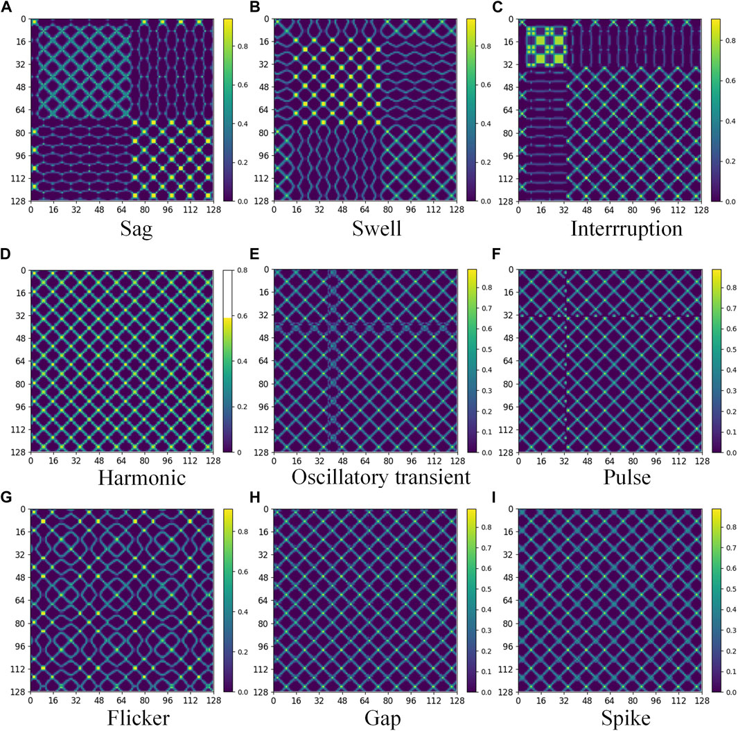
FIGURE 2. MTF visualization image of PQDs basic signals.

As depicted in Figure 2, the MTF feature image differentiates time-series signals of various PQDs types at the same spatial location by employing dissimilarities in pixel colors and texture shapes. The feature information of each image is lucid and easily distinguishable, thereby facilitating feature extraction after disturbances composite superposition, and laying a foundation for deep learning network to accurately recognize PQDs.

3 PQDs recognition based on improved DenseNet

3.1 Fundamental principle of DenseNet

Traditional CNNs come with an abundance of parameters and frequently encounter two primary issues: first, overfitting is easy to occur owing to limited training data, and second, the network layers tend to be shallow, causing inadequate extraction of more advanced information. Deeper networks produce more distinguishable characteristics by acquiring superior-level feature maps, thus it’s easier for them to recognize inherent and underlying features. However, deep neural networks often encounter issues such as gradient vanishing and explosion, which can negatively impact network training and recognition performance (Huang et al., 2017b).

DenseNet incorporates a bypass connection approach similar to ResNet and establishes a dense connection mechanism between convolutional layers, enhancing feature reuse through inter-channel splicing (Huang et al., 2017a). As a result, DenseNet effectively resolves the aforementioned issues. As its core component module, the dense block (DB) structure as depicted in Figure 3, which is designed to ensure maximum information flow between network layers, where: $x_0$ is the input feature information, the input of $H_1$ is $x_0$, while the inputs of $H_2$ are $x_0$ and $x_1$, where $x_1$ is the output of $H_1$, and so on. In this architecture, each layer uses inputs from all previous layers and passes its corresponding feature maps to all subsequent layers. Therefore, this network structure can extract more global and important features, which can achieve more accurate and efficient training effect.

FIGURE 3

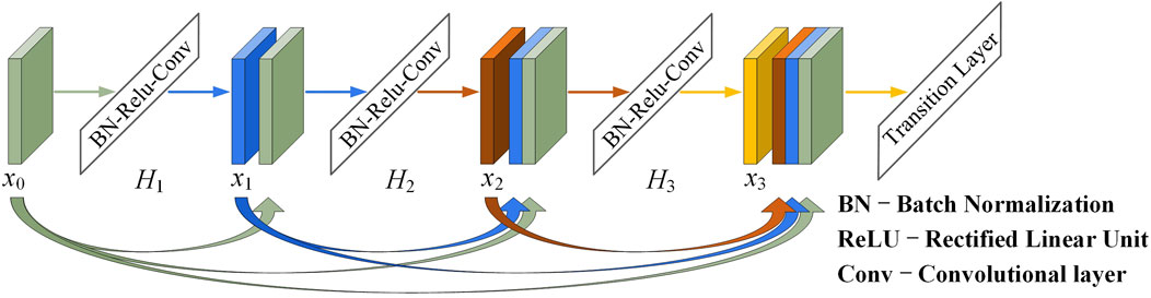
FIGURE 3. A dense block structure.

Unlike the conventional convolutional network structure, the number of connections increases to $L\left(L+1\right)/2$ from L when the number of DB layers is $L$. As a result, the feature map obtains from the $L$-th layer is the outcome of the feature maps that are produced from all previous layers after being spliced in the channel dimension using the following Eq. 3:

$x_l=H_l\left(\left[x_0,x_1,\dots ,x_{l-1}\right]\right)(3)$

where $x_l$ represents the output of layer $l$. The splicing operation of the output feature map of each layer is denoted by $\left[x_0,x_1,\dots ,x_{l-1}\right]$. $H_l\left(\bullet \right)$ represents a nonlinear combinatorial function, which consists of a batch normalization layer (BN), a linear activation function (ReLU), and a $3\times 3$ convolutional layer (Conv).

Each DB includes multiple convolutional layer structures with the same padding utilized for splicing operations. Although this structure adopts a densely connected pattern, it requires fewer parameters than traditional CNNs. In fact, this network architecture eliminates the need to learn redundant information, reduces the number of feature maps required at the network layer, and significantly improves parametric efficiency. On the other hand, the continuous concatenation of different layers requires each layer to access the gradient from the original input data and the loss function. This fast access improves the information flow between layers, mitigates the gradient vanishing issue, and facilitates the extraction of deeper semantic information.

3.2 Foundational network architecture design

To avoid overfitting and create a more lightweight network, this paper designs a more compact and lightweight architecture termed DenseNet-S through numerous experimental tests. This architecture serves as the backbone of deep learning network while ensuring the network’s classification precision. Its network structure is shown in Table 2. Among them, the DenseNet-S network contains four groups of DBs, each group is composed of 3, 6, 9, and 6 groups of convolutional layer superposition connections, and the growth rate $k=48$. To enhance the network’s computational efficiency and compactness, bottleneck layer and transition layer are introduced for feature map dimensionality reduction. The bottleneck layer is located in DB and consists of $1\times 1$ convolutional layers preceding $3\times 3$ convolutional layers. The transition layer is located between two sets of DBs and consists of a batch normalization layer, a $1\times 1$ convolutional layer, and a $2\times 2$ average pooling layer. For $m$ feature maps output by DB, $\theta$ times will be reduced after conversion by transition layer. $\theta \in \left(0,1\right)$ is the compression coefficient. In this paper, we use $\theta =0.5$.

TABLE 2

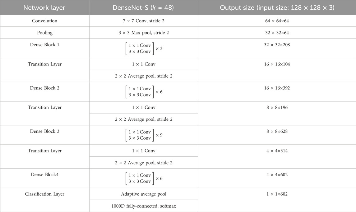
TABLE 2. Network structure design of DenseNet-S.

3.3 CBAM attention mechanism

Accurate extraction of feature image information is crucial for improving the recognition accuracy of PQDs. The convolutional and pooling operation of CNNs defaults the importance of each channel in the feature map to be the same, but due to the different importance of information carried, it is unreasonable to identify the same importance of channels. Based on the processing mechanism of the human visual system, CBAM (Woo et al., 2018) performs dynamic weighted processing of features through autonomous learning on spatial domains and feature channels to enhance the capture of key feature information of images while reducing the interference of non-key information, thus improving the recognition precision. Therefore, this paper introduces CBAM attention mechanism to improve the ability of feature extraction network to focus details in MTF images corresponding to various PQDs, so as to obtain better recognition effect.

CBAM comprises two modules: channel attention module (CAM) and spatial attention module (SAM). CAM assigns weight coefficients to the feature channels based on their significance. Firstly, all channels information is aggregated through average-pooling and max-pooling to generate two different one-dimensional feature vectors, and then, after fully connected layer operation, element by element addition is performed, channel attention weight $M_c$ is generated through activation operation, which is then multiplied element by element with the input feature map to obtain the channel attention weighted feature map $F_1$. The calculation process of CAM module is shown in Figure 4A, and its calculation expression is shown in Eq. 4:

$M_C\left(F\right)=\sigma \left(\text{MLP}(\text{AvgPool}\left(F\right)\right)+\text{MLP}\left(\text{MaxPool}\left.\left(F\right)\right)\right)(4)$

where $F$ represents the input feature map, $\text{AvgPool}$ and $\text{MaxPool}$ indicate average-pooling and max-pooling operations, respectively. $\text{MLP}$ denotes the fully connected operation, while $\sigma$ represents the sigmoid function.

FIGURE 4

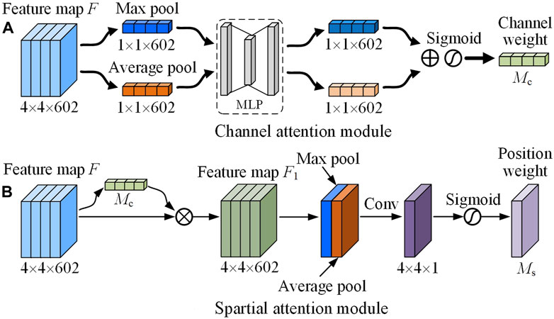
FIGURE 4. Schematic diagram of CBAM.

The SAM module uses the feature map $F_1$ as the input, which has been weighted by CAM. As shown in Figure 4B, the input feature map $F_1$ undergoes spatially max-pooling and average-pooling resulting in two two-dimensional feature maps, which are splicing for convolution operation and activation operation, and finally generates spatial attention weight $M_s$ to obtain features weighted by SAM. The formula for calculating the spatial attention is shown in Eq. 5:

$M_S\left(F\right)=\sigma (f^{3\times 3}\left(\left[\text{AvgPool}\left(F\right);\text{MaxPool}\left(F\right)\right]\right))=\sigma (f^{3\times 3}\left(\left[F_{\text{avg}}^S;F_{\mathit{max}}^S\right]\right))(5)$

where $f^{3\times 3}$ represents the dimensionality reduction convolution operation with a convolution kernel size of $3\times 3$. (The study discovers that using $3\times 3$ convolution kernel size for dimensionality reduction of feature channel results in better intelligent network recognition performance than $7\times 7$ convolution kernel size. Therefore, the convolution operation with the kernel size of $3\times 3$ is utilized here).

3.4 PQDs recognition framework construction

Combining the imaging advantages of MTF with DenseNet’s efficient training and deep feature extraction capabilities, this paper proposes a novel PQDs recognition method based on MTF and improved DenseNet. The PQDs recognition framework is shown in Figure 5. The whole framework mainly includes four parts: signal visualization module, dense connection learning module, attention mechanism module and classification module.

(1) Signal visualization module: The one-dimensional PQDs time-series sampling signals are deconstructed through MTF dynamic coding, reorganized into MTF matrix to retain the original temporal information. Finally, the matrix is mapped into a two-dimensional image with easy-to-recognize features and temporal correlation, having a pixel size of $128\times 128$. This approach indirectly enhances the recognition precision of disturbance types from the data level.

(2) Dense connection learning module: This module comprises DBs and transition layers. RGB feature maps undergo convolution and dimension reduction via $7\times 7$ convolution layers and $3\times 3$ max-pooling layers to extract shallow feature information. Following feature extraction, the feature information needs to traverse four sets of DBs, with a transition layer connecting every two sets of DBs. When passing through DBs, feature reuse is performed on feature maps from different layers in channel dimension based on dense connection mechanism, which is conducive to extracting deeper feature information and combining shallow layer and deep layer information in the network, which greatly improves feature utilization. Simultaneously, transition layers are introduced to reduce feature dimensions, which reduces network parameter redundancy and enhances the overall efficiency of the model’s learning and computation.

(3) Attention mechanism module: Adding the CBAM attention module between the dense connection learning module and the classification module of DenseNet-S can effectively enhance the network’s recognition precision, as evidenced by extensive experimentation. The feature map $F$ output by Dense Block 4 enters the CAM module, where max-pooling and average-pooling operations are performed and result in two $1\times 1\times 602$ one-dimensional feature vectors. Then the two feature vectors are sent into the full connection layer for calculation and sum operation. After activation operation, the CAM module generates channel attention weights $M_c$, which are then multiplied with the feature map $F$ to derive $F_1$ that is the input feature map for the SAM module. In the SAM module, the feature map $F_1$ undergoes separate max-pooling and average-pooling operations according to spatial position, and the two results are splicing to generate a $4\times 4\times 2$ feature map. Subsequently, this map undergoes dimensional reduction through a 1-channel convolution layer. The spatial attention weight $M_s$ is then obtained by Sigmoid function activation. Ultimately, the feature obtained by multiplying the weights $M_s$ with the input feature map $F_1$ represents the feature enhanced by CBAM.

(4) Classification Module: This module consists of an adaptive average-pooling layer, two fully connected layers, and a Softmax classifier. Firstly, the feature maps enhanced by CBAM are converted into one-dimensional feature vectors using adaptive average pooling, which is then input into the fully connected layer. Finally, the feature information output from the fully connected layer is input into the Softmax classifier. Softmax function is used to calculate the probability value of each PQDs type corresponding to the MTF feature image, and the category of the maximum value is output as the classification result to realize the recognition of PQDs type.

FIGURE 5

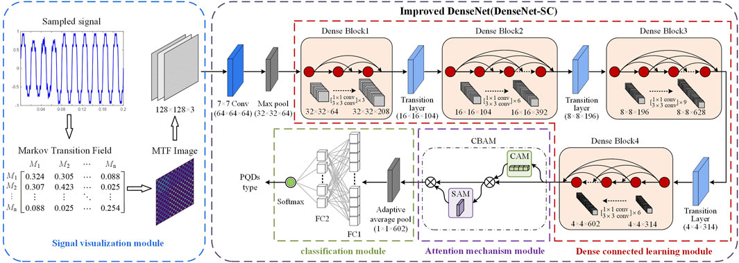
FIGURE 5. PQDs recognition framework based on MTF and improved DenseNet.

4 Simulation analysis

4.1 PQDs visualization dataset generation

According to IEEE Std 1159–2019, 34 composite disturbances are generated by combining nine mathematical models of basic disturbance signals. These composite disturbances included 18 double disturbances, 11 triple disturbances, and 5 quadruple disturbances. The random parameters of PQDs including fluctuation amplitude and duration are based on Table 1. Additionally, in alignment with Section 2.3’s outlined signal sampling parameters, 1,000 samples are generated for each disturbance with uniform amplitude and phase distribution. These samples are produced at varying signal-to-noise ratios (SNRs) of 0 dB, 20 dB, 30 dB, and 50 dB to better simulate real-world PQDs scenarios. Through the visual conversion process of PQDs signal in Section 2.3, MTF is used to map samples into two-dimensional images, and a total of 43 types of PQDs visualization dataset is constructed.

This paper presents the development of a PQDs recognition model utilizing the PyTorch deep learning framework in Python 3.9. The experimental environment uses AMD Ryzen 3,970X @ 3.70 GHz CPU, 128 GB RAM, and NVIDIA RTX 3090 GPU. The cross-validation technique is used in the training process. In each epoch, the data from all categories are randomly arranged and divided into training, validation, and test sets according to the ratio of 6:2:2, and the optimal model is saved according to the recognition accuracy of validation sets.

4.2 Model parameter settings and evaluation criteria

When training the PQDs recognition model, the batch size is set to 64, the number of training epochs is set to 50, and the initial learning rate is set to 0.001. In order to obtain the optimal training model, the stochastic gradient optimizer (SGD, weight_decay = 0.0001, momentum = 0.9) is used to optimize the model, and the cross entropy loss function is used to calculate the loss value. To ensure the network learning efficiency and prevent overfitting, a dynamic adjustment strategy is used to update the learning rate. After 50% of the total epochs are completed, the learning rate is adjusted to the original 10%.

To evaluate the model’s performance, this paper uses multiple evaluation metrics such as average recognition accuracy (Accuracy), floating-point operations (FLOPs), parameters (Params), and model size. Accuracy is calculated using the subsequent Eq. 6: The formula for calculating the spatial attention weights is as follows:

$\text{Accuracy}=\frac{1}{N}{\displaystyle \sum _{j=1}^n}\frac{M_{jj}}{M_j}\times 100\%(6)$

where $N$ is the total number of categories, $M_j$ is the number of the $j$-th category, and $M_{jj}$ is the number of correct recognition for the $j$-th category.

Params and FLOPs in CNNs are widely used to evaluate the complexity of the model (Paoletti et al., 2021). The formulas is calculated using the subsequent equation: for calculating Params and FLOPs in the convolution layer and the fully connected layer are as Eqs 7–10:

$P_{CNN}\sim O\left({\displaystyle \sum _{l=1}^d}\left(n_{l-1}\bullet s_l^2+1\right)\bullet n_l\right)(7)$

$C_{CNN}\sim O\left({\displaystyle \sum _{l=1}^d}{n}_{l-1}\bullet s_l^2\bullet n_l\bullet m_l^2\right)(8)$

$P_{FCN}\sim O\left({\displaystyle \sum _{l=1}^d}\left(n_{l-1}+1\right)\bullet n_l\right)(9)$

$C_{FCN}\sim O\left({\displaystyle \sum _{l=1}^d}{n}_{l-1}\bullet n_l\right)(10)$

where $l$ is the index of a convolutional layer, and $d$ is the depth (number of convolutional layers). $n_l$ is the number of filters (also known as “width”) in the $l$-th layer. $n_{l-1}$ is also known as the number of input channels of the $l$-th layer. $s_l$ is the spatial size (length) of the filter. $m_l$ is the spatial size of the output feature map.

4.3 Experimental results and analysis

In order to verify the performance of the improved DenseNet-SC model designed in this paper in recognizing PQDs types, the improved model is compared with the DenseNet-S model and six mainstream deep learning classification networks under the same experimental environment and SNR conditions, so as to verify the effectiveness and superiority of the improved model.

4.3.1 DenseNet-SC model capability assessment

The improved DenseNet-SC model and the DenseNet-S model without CBAM module are trained with the same dataset and experimental environment. After 50 epochs of training, the recognition accuracy and loss value changes of the verification set in the training process of the model are obtained, as shown in Figure 6. At the same time, comparison results of various models’ recognition accuracy on the test set can be obtained under different SNR environments, among which the overall recognition accuracy of DenseNet-S is 95.72%, 95.06%, 93.92%, and 89.72% under no noise, 50 dB, 30 dB, and 20 dB environments, respectively. In the identical SNR environments, the overall recognition accuracy of DenseNet-SC is 98.29%, 97.64%, 96.80%, and 93.26%, respectively.

FIGURE 6

FIGURE 6. Comparison of recognition results on validation set.

As can be seen from Figure 6, the accuracy and convergence rate of the improved DenseNet-SC model are significantly better than that of the DenseNet-S model during the epochs. Once it reaches the state of convergence, the accuracy of the former is stable at about 98%, and the loss value is stable at about 0.07, while the accuracy and loss value of the latter are oscillating at about 95% and 0.17, respectively. This suggests that the addition of CBAM module to the DenseNet-S model effectively improves the extraction of detailed features in the MTF images that correspond to PQDs signals, so as to grasp the feature information in the input image more accurately. By comparing the overall recognition results of the two models on the test set, it can be seen that the DenseNet-SC model also performs better than DenseNet-S in PQDs recognition under four noise environments: no noise, 50 dB, 30 dB, and 20 dB. The recognition accuracy is improved by 2.57, 2.58, 2.88, and 3.54 percentage points respectively, which further indicates that adding CBAM attention mechanism between the dense connection learning module and the classification module of model is more helpful for the model to focus on key feature information, so as to improve the recognition performance.

The Grad-Cam method (Selvaraju et al., 2020) showcases the degree to which different network modules concentrate on image features via a heatmap. The heatmap’s colorbar value indicates the degree of network focus, with higher values indicating a greater level of focus. The class activation heatmaps of the output features of some samples before and after CBAM module by the improved model are shown in Figure 7. The figure indicates that, regardless of basic, double, triple, or quadruple disturbances, the image areas of focus are more precise and comprehensive in capturing key texture features in the MTF images when passing through the CBAM module than when passing through the dense connection learning module. The reason for this is that the deeper features of feature extraction module are more related to global information, and the CBAM module assigns more weight coefficients to the network from a global viewpoint. Therefore, deep global features can be better extracted and learned through CBAM module, which enables the focused feature areas to cover the MTF texture pattern areas with key feature information more comprehensively.

FIGURE 7

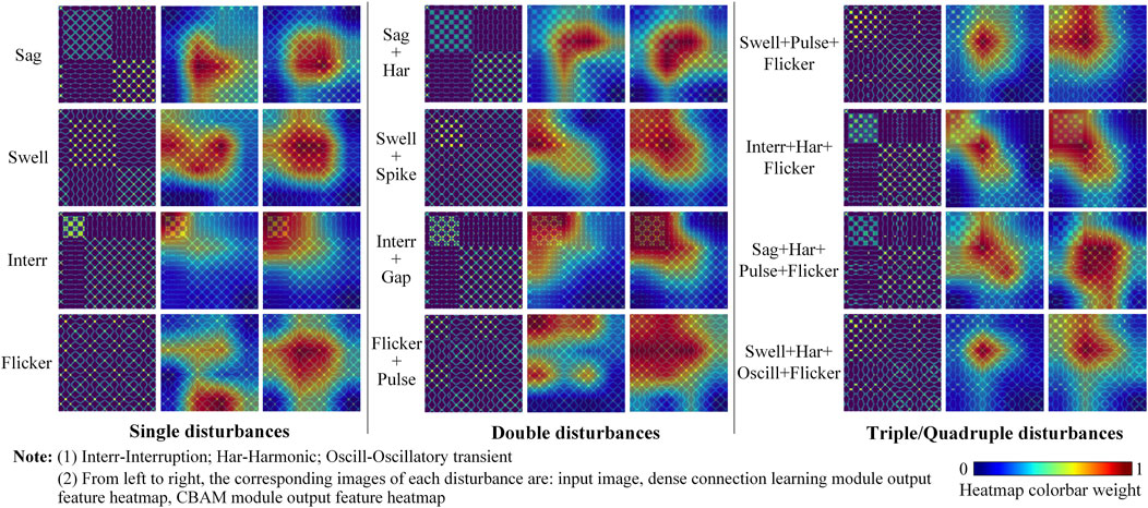
FIGURE 7. Comparison of the class activation heatmap output before and after the CBAM module of improved model.

4.3.2 Model noise resistance performance evaluation

In noisy environments, PQDs signals may become distorted, potentially interfering with the model’s judgment of their real class and causing a reduction in the network’s recognition precision. To evaluate the anti-noise ability of the improved model, combined with the model recognition performance under different SNR environments in the previous section, the recognition effect on various types of disturbances is tested respectively in the 20 dB SNR environment. The corresponding confusion matrix of the test results is shown in Figure 8, where the rows indicate the actual disturbance labels while the columns reflect the model’s recognition outcomes.

FIGURE 8

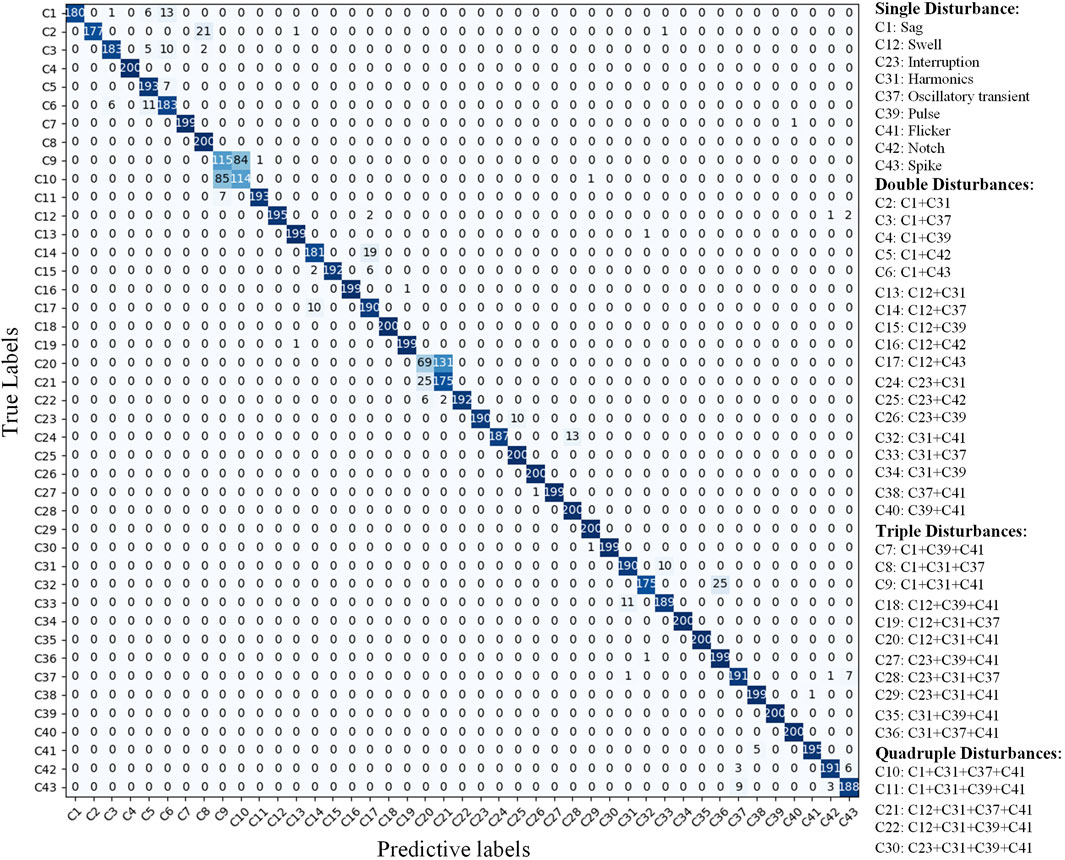
FIGURE 8. Confusion matrix of 43 types PQDs recognition results (SNR = 20 dB).

The test results show that under the 20 dB strong noise environment, the recognition accuracy of some complex disturbances containing oscillatory transient, harmonic, flicker and spike, is below average. Among them, some disturbances are easily confused with complex disturbances containing notch and spike $\left(\mathrm{C}1\to \mathrm{C}5/\mathrm{C}6,\mathrm{C}3\to \mathrm{C}5/\mathrm{C}6,\mathrm{C}14\to \mathrm{C}17\right)$. Some double disturbances with harmonic can be easily identified as triple disturbances $\left(\mathrm{C}2\to \mathrm{C}8,\mathrm{C}24\to \mathrm{C}28,\mathrm{C}32\to \mathrm{C}36\right)$ and the quadruple disturbances with oscillatory transient are easily confused with the triple disturbances without oscillatory transient $\left(\mathrm{C}9\to \mathrm{C}10,\mathrm{C}20\to \mathrm{C}21\right)$, resulting in a significant decline in recognition accuracy. On the other hand, the overall recognition accuracy of the improved model can still reach 93.26% even under 20 dB strong noise environment, which shows good recognition performance and noise robustness.

4.3.3 Comparison of recognition precision performance among different deep learning models

To further verify the precision performance of DenseNet-SC model in recognizing PQDs, we performed comparative experiments with six mainstream deep learning classification networks: GoogleNet (Inception V3), Vgg-16, ResNet-18, and DenseNet-121/169/201 under equivalent conditions of MTF dataset and experimental settings. These classification networks utilize the corresponding framework structure and parameters setting from the original papers. Figure 9 shows the comparison curves of recognition accuracy, while Table 3 presents the recognition accuracy results on the test set. It is important to note that MTF images need to be upsampled to $299\times 299$ and $224\times 224$ respectively before being input into the networks so as to adapt to the pre-trained GoogleNet and the other five classification networks, while the proposed DenseNet-SC does not require any prior information.

FIGURE 9

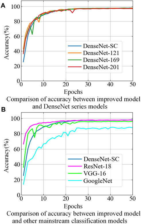
FIGURE 9. Comparison of recognition accuracy between DenseNet-SC and matinstream deep learning networks.

TABLE 3

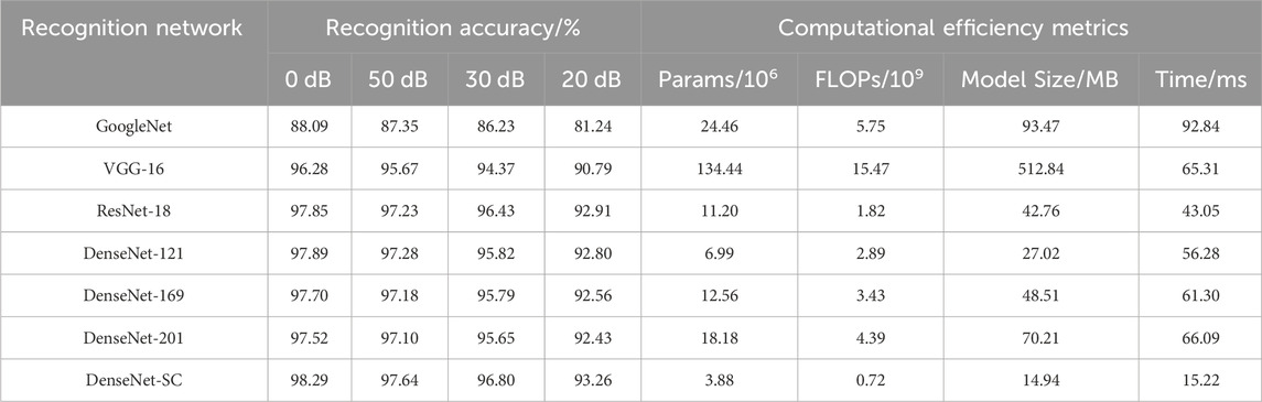
TABLE 3. Comparison of recognition performance on Test set.

As shown in Figure 9A, compared with the three DenseNet series classification networks, although the initial recognition accuracy of the improved model is relatively low, its accuracy continues to increase and the rising trend is very stable with the increase of epochs, and there is no obvious fluctuation. In the 16th epoch, the initial synchronization with other models is achieved, and the surpassing is completed in the later stage. In addition, as can be seen from Table 3, the recognition accuracy of the improved model under different SNR environments is superior to the other three models in terms of accuracy performance verification of the test set. In summary, although DenseNet-SC model is lightweight in the network architecture, the increase in growth rate and the injection of CBAM attention module strengthen the propagation of feature information and the extraction of key features, improve the information flow and feature capture capability of the whole network, and optimize its recognition precision performance for PQDs.

According to Figure 9B; Table 3, GoogleNet underperforms on the MTF dataset. Its recognition accuracy is lower than that of other models in both training and testing phases. Compared with VGG-16 and ResNet-18 models, on the one hand, although the improved model exhibits subpar performance during the early training phase, the recognition accuracy gradually exceeds that of two models with the increase of epochs, and finally stabilizes around 98%. On the other hand, in terms of test performance, the overall recognition accuracy of the improved model under the SNR of 0, 20, 30, and 50 dB is improved by 2.01/0.44, 1.97/0.41, 2.43/0.37, and 2.47/0.35 percentage points compared with the two models, respectively. These results demonstrate the improved model’s superiority in terms of PQDs recognition precision and noise resistance.

4.3.4 Comparison of recognition efficiency performance among different deep learning models

Considering the high requirement of PQDs recognition efficiency for power system health status monitoring, the size of recognition model and its operational efficiency are important evaluation metrics to judge its performance. The size and operational performance of different recognition models are shown in Table 3, where time refers to the average time of taking the model to recognize a sample image from the test set over 100 tests.

As can be seen from Table 3, when compared with ResNet-18 and the three DenseNet series models, the recognition accuracy of Densenet-SC model improves relatively little, but the number of Params, FLOPs, model size and recognition time are greatly reduced. Among them, the Params and the model size of DenseNet-SC are only 55.51% of DenseNet121 model, which is the lightest model among the six comparison models, while the FLOPs and the recognition time to recognize an image are less than 40% of ResNet-18 model, which has the highest operational efficiency among the comparison models. This can not only effectively reduce the memory ratio and computing power, but also help to improve the training and testing efficiency of the model, so as to realize the PQDs recognition operation performance upgrade of the model. On the other hand, compared with the GoogleNet and VGG-16 models, the proposed model has achieved significant optimization in terms of recognition accuracy, model size and computing performance. In addition, due to the influence of input image size and its own network structure, GoogleNet’s efficiency of recognizing an image is lower than that of VGG-16. To sum up, the DenseNet-SC model designed in this paper not only improves the network recognition precision, but also realizes the lightweight and high efficiency of the network, making it able to be deployed on the hardware terminal equipment with small storage capacity and low computing performance configuration, which provides the possibility for further exploring the construction of mobile PQDs recognition system.

5 Real-world field measured signals analysis

5.1 Practical effectiveness analysis of the proposed PQD recognition method

To assess the effectiveness of the proposed method for practical engineering use, real-world field measured PQDs signal data is utilized to test its recognition performance. The data used for testing are gathered from a power quality monitoring device in a 10 kV substation located in the southern region of Jiangsu Province, China. The data collection period ranges from March 2020 to August 2021, comprising a total of 181 sets of samples. The recording device has a sampling frequency of 12.8 kHz and the signal lasted for 0.624 s. To conform with IEEE Std1159-2019 and the input requirements of the proposed recognition network, the 10-cycle typical data of each set of signals is intercepted and normalized as the input of signal visualization module. The real-world field measured waveforms of PQDs typical events and their MTF conversion images are shown in Figure 10. It can be seen that the MTF image corresponding to each disturbance measured signal still have clear and easily distinguishable texture pattern features, which are basically consistent with the theoretical MTF image features. Therefore, it can be seen that the MTF conversion mode also has good feature expression ability for the real-world field measured signal data. MTF samples corresponding to all measured signals are identified by the DenseNet-SC optimal training model, and the results are shown in Table 4.

FIGURE 10

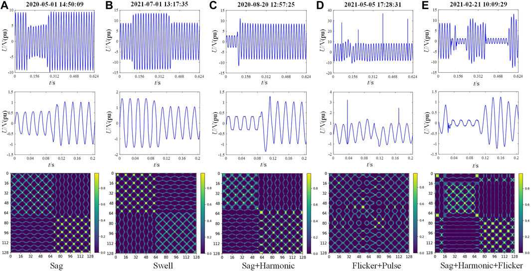
FIGURE 10. Real-world field measured waveform and MTF conversion diagram of typical PQDs event.

TABLE 4

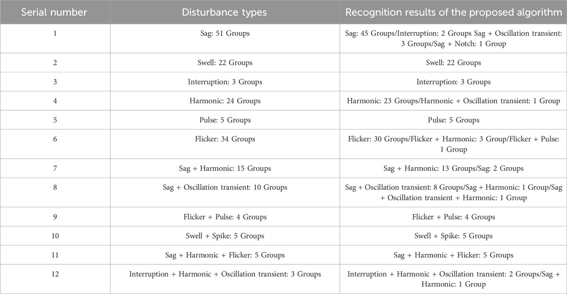
TABLE 4. Recognition results of real-world field measured PQDs signal.

As can be seen from Table 4, in terms of sag recognition, 2 groups are recognized as interruption due to the too low sag amplitude of signal sequence, and 4 groups are recognized as sag + oscillatory transient/notch due to environmental noise interference. In terms of flicker recognition, 3 groups are detected to contain harmonic components due to the influence of noise, and 1 group is identified to contain pulse disturbance due to the presence of serious noise point. In terms of double disturbance recognition, the two groups of sag + harmonic are identified as sag. Further analysis shows that the harmonic content in the measured signal is small and its total proportion is relatively small, resulting in label loss. In addition, a group of triple disturbance signals (interruption + harmonic + oscillatory transient) are recognized as sag + harmonic because the signal sag amplitude is near the critical value and the oscillatory amplitude is relatively small. In summary, due to the mismatch between the real-world field measured signal data and the simulation signal data simulated by mathematical model, the recognition accuracy of some measured disturbance types decreases compared with the simulation results, but on the whole, the measured disturbance signal types can be effectively recognized with a high precision of 91.16%. Therefore, the effectiveness and reliability of the proposed method in engineering practice are verified.

5.2 Comparative performance analysis with existing PQDs recognition frameworks

To further verify the comprehensive performance advantages of the proposed method in terms of efficiency and accuracy, six existing PQDs identification algorithms that have achieved excellent performance are selected as benchmark algorithms for comparative analysis with the proposed algorithm on the real-world field measured dataset. The benchmark algorithms are divided into machine learning algorithms and deep learning algorithms.

The machine learning algorithms include DWT + PNN (Khokhar et al., 2017) and ST + RBF (Wang et al., 2018), while the deep learning algorithms include the one-dimensional deep learning algorithms GRU (Deng et al., 2019) and LSTM (Xu et al., 2022), which directly take one-dimensional signals as model inputs, and the two-dimensional deep learning algorithms GASF + CNN (Zheng et al., 2021) and GASF-GADF + ResNet18, which convert one-dimensional signals into two-dimensional visualization images and then combine advanced image recognition algorithms for PQDs classification.

To ensure the fairness of various algorithms in the PQDs recognition performance test, we process the data and train the classifier models based on the same original one-dimensional signal dataset under the same experimental environment. Among them, the original dataset is divided according to the same dataset partitioning ratio as in this paper, the classifier model structure is consistent with that in the original paper, and the hyperparameter settings are consistent with that in this paper. After the training of various algorithm models and saving the optimal models, they are applied to the measured signal dataset and the comprehensive performance is compared with the proposed method. The results are shown in Figure 11. Among them, the visual conversion and network classification time are the average time obtained for a signal sample after 100 consecutive tests. Sequence conversion time and network classification time refers to the average time used to process and recognize a signal sample in the dataset, respectively.

FIGURE 11

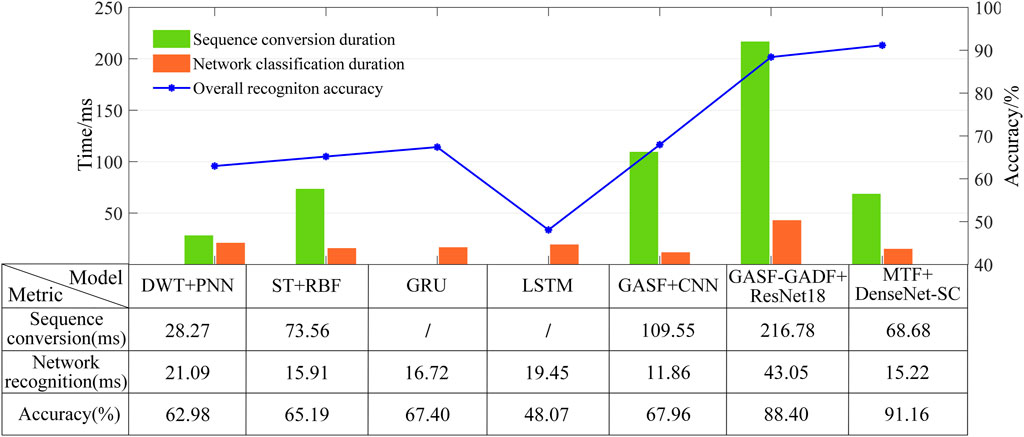
FIGURE 11. Comparison of precision and efficiency metrics of different PQDs recognition frameworks.

According to the test results, the overall accuracy performance of machine learning algorithms is poor. This is because this algorithm type relies heavily on expert knowledge when manually extracting features, and its generalization performance is greatly limited when facing measured signals with more complex changing states. In addition, machine learning models often have shallow depth, which leads to their lack of deep feature capture ability, thereby causing a decline in PQDs recognition accuracy performance. One-dimensional deep learning algorithms directly take one-dimensional sequence data as model input without any data processing, so they are superior to other algorithms in efficiency performance. However, their accuracy performance is limited due to its limitation in information mining of complex time series data. With the deep feature mining ability and strong generalization of advanced image recognition algorithms, the accuracy performance of two-dimensional deep learning algorithms is better than that of traditional machine learning algorithms and one-dimensional deep learning algorithms. Among them, due to the limited temporal and spatial features of the PQDs signals extracted by single-channel GASF in the coding process, and the shallow depth of CNN network, the deep-level semantic information of the image cannot be captured, thus the overall recognition accuracy of GASF + CNN is only 67.96%. Compared with single-channel GASF, double-channel GASF-GADF can provide more abundant PQDs time-series feature information. However, real-world disturbance signal aliases environmental noise and its state changes are more complex, which makes the GAF visualization process requiring coordinate conversion and matrix coding inevitably lose some important feature information. It interferes with the classification network to capture important feature information, and then reduces the recognition performance of the model, so its accuracy is also limited. Compared with GAF, MTF is more resistant to interference and noise through the introduction of quantile division, and the encoded image obtained by conversion can retain more comprehensive temporal and spatial feature information. In terms of recognition efficiency, the visual conversion efficiency of the proposed method is much higher than other two methods, because the MTF conversion process is very simple and computationally small, and it does not need to carry out complex coordinate conversion and matrix coding. In addition, due to the lightweight structural design, the model recognition efficiency is higher than that of the larger ResNet-18, but it is lower than that of CNN, because CNN has a simpler structure (the number of parameters and the model size are 2.18 M and 8.32 MB, respectively). However, CNN has obvious defects in the recognition accuracy performance. In summary, the experimental results of measured signals prove that the MTF + DenseNet-SC method proposed in this paper has better comprehensive performance in PQDs recognition than other algorithms.

6 Conclusion

To meet the recognition efficiency and precision requirements of massive and complex PQDs events under the background of new power system, and give full play to the deep sensing capability of DenseNet and the simple conversion and anti-interference capability of MTF, a novel PQDs recognition method based on MTF and improved DenseNet is proposed in this paper. The specific advantages are as follows:

1) MTF can effectively extract the disturbance characteristics of one-dimensional signals, and has certain anti-interference ability. The two-dimensional images after visualization can effectively express the sample disturbance information.

2) A DenseNet-S lightweight network structure is designed, and by introducing an attention mechanism, the improved model can capture the texture pattern features of each MTF sample more accurately and comprehensively. The recognition accuracy of 43 PQDs types can reach 98.29% and 93.26% respectively under noise-free and 20 dB strong noise environment, which effectively improves the PQDs recognition precision and noise robustness.

3) The improved DenseNet-SC model has obvious advantages over six mainstream deep learning image classification models, such as ResNet-18 and DenseNet-121, in terms of model size, Paras, FLOPs and recognition time. While improving recognition precision, the lightweight of model and the high efficiency of data analysis are realized. In addition, this paper constructs 12 types of real-world field measured PQDs signal dataset to comprehensively test the recognition performance of the proposed method. The test results verify the effectiveness and superiority of the proposed method in the accuracy and efficiency of real-world field measured PQDs recognition, which can meet the classification accuracy and efficiency requirements of massive and complex PQDs events in engineering applications.

Data availability statement

The original contributions presented in the study are included in the article/Supplementary material, further inquiries can be directed to the corresponding author.

Author contributions

LZ: Conceptualization, Formal Analysis, Investigation, Methodology, Validation, Writing–original draft. SG: Data curation, Investigation, Resources, Validation, Writing–review and editing. YL: Resources, Supervision, Validation, Writing–review and editing. CZ: Resources, Software, Supervision, Writing–review and editing.

Funding

The author(s) declare financial support was received for the research, authorship, and/or publication of this article. This work was supported by the State Grid Jiangsu Electric Power Co., Science and Technology Project (J2022093).

Conflict of interest

Authors LZ, SG, YL, and CZ were employed by State Grid Suzhou Power Supply Company.

Publisher’s note

All claims expressed in this article are solely those of the authors and do not necessarily represent those of their affiliated organizations, or those of the publisher, the editors and the reviewers. Any product that may be evaluated in this article, or claim that may be made by its manufacturer, is not guaranteed or endorsed by the publisher.

References

Ahmadi, A., and Tani, J. (2019). A novel predictive-coding-inspired variational RNN model for online prediction and recognition. Neural Comput. 31 (11), 2025–2074. doi:10.1162/neco_a_01228

PubMed Abstract | CrossRef Full Text | Google Scholar

Cui, C. H., Duan, Y. J. V., Hu, H. l., Wang, L., and Liu, Q. (2022). Detection and classification of multiple power quality disturbances using stockwell transform and deep learning. IEEE Trans. Instrum. Meas. 71, 1–12. doi:10.1109/TIM.2022.3214284

CrossRef Full Text | Google Scholar

Deng, Y., Wang, L., Jia, H., Tong, X., and Li, F. (2019). A sequence-to-sequence deep learning architecture based on bidirectional GRU for type recognition and time location of combined power quality disturbance. IEEE Trans. Industrial Inf. 15 (8), 4481–4493. doi:10.1109/TII.2019.2895054

CrossRef Full Text | Google Scholar

He, C. J., Li, K. C., and Yang, W. W. (2023). Power quality compound disturbance identification based on dual channel GAF and depth residual network. Power Syst. Technol. 47 (1), 369–376. doi:10.13335/j.1000-3673.pst.2022.0644

CrossRef Full Text | Google Scholar

Huang, G., Liu, Z., Van, D. M., and Weinberger, K. Q. (2017b). Densely connected convolutional networks. Proc. CVPR, 4700–4708. doi:10.1109/CVPR.2017.243

CrossRef Full Text | Google Scholar

Huang, J. M., Ju, H. Z., and Li, X. M. (2016). Classification for hybrid power quality disturbance based on STFT and its spectral kurtosis. Power Syst. Technol. 40 (10), 3184–3191. doi:10.13335/j.1000-3673.pst.2016.10.036

CrossRef Full Text | Google Scholar

Huang, N. T., Peng, H., and Cai, G. W. (2017a). Feature selection and optimal decision tree construction of complex power quality disturbances. Proc. CSEE 37 (3), 776–785. doi:10.13334/j.0258-8013.pcsee.160108

CrossRef Full Text | Google Scholar

Jyoti, S., Basanta, K. P., and Prakash, K. R. (2021). Power quality disturbances classification based on Gramian angular summation field method and convolutional neural networks. Int. Trans. Electr. Energy Syst. 31 (12), e13222. doi:10.1002/2050-7038.13222

CrossRef Full Text | Google Scholar

Khokhar, S., Zin, A. A., Memon, A. P., and Mokhtar, A. S. (2017). A new optimal feature selection algorithm for classification of power quality disturbances using discrete wavelet transform and probabilistic neural network. Measurement 95 (2017), 246–259. doi:10.1016/j.measurement.2016.10.013

CrossRef Full Text | Google Scholar

Li, D. Q., Mei, F., Zhang, C. Y., Sha, H. Y., Zheng, J. Y., and Li, T. R. (2020). Deep belief network based method for feature extraction and source identification of voltage sag. Automation Electr. Power Syst. 44 (04), 150–160. doi:10.7500/AEPS20190306004

CrossRef Full Text | Google Scholar

Li, R. J., W, Y., Wu, Q., Nilanjan, D., Rubén, G. C., and Shi, F. Q. (2022). Emotion stimuli-based surface electromyography signal classification employing Markov transition field and deep neural networks. Measurement 189 (2022), 110470. doi:10.1016/j.measurement.2021.110470

CrossRef Full Text | Google Scholar

Paoletti, E. M., Haut, M. J., Tao, X. W., Plaza, J., and Plaza, A. (2021). FLOP-reduction through memory allocations within CNN for hyperspectral image classification. IEEE Trans. Geoscience Remote Sens. 59 (7), 5938–5952. doi:10.1109/TGRS.2020.3024730

CrossRef Full Text | Google Scholar

Selvaraju, R. R., Cogswell, M., Das, A., Vedantam, R., Parikh, D., and Batra, D. (2020). Grad-CAM: visual explanations from deep networks via gradient-based localization. Proc. ICCV, 618–626.

CrossRef Full Text | Google Scholar

Sindi, H., Nour, M., Rawa, M., Öztürk, Ş., and Polat, K. (2021). An adaptive deep learning framework to classify unknown composite power quality event using known single power quality events. Expert Syst. Appl. 178, 115023. doi:10.1016/j.eswa.2021.115023

CrossRef Full Text | Google Scholar

Std (2019). IEEE recommended practice for monitoring electric power quality. IEEE 29, 240. 01-Power transmission and distribution networks in general.

Google Scholar

Tang, Q., Qiu, W., and Zhou, Y. C. (2020). Classification of complex power quality disturbances using optimized S-transform and kernel SVM. IEEE Trans. Industrial Electron. 67 (11), 9715–9723. doi:10.1109/TIE.2019.2952823

CrossRef Full Text | Google Scholar

Wang, F., Quan, X. Q., and Ren, L. T. (2021). Review of power quality disturbance detection and identification methods. Proc. CSEE 41 (12), 4104–4120. doi:10.13334/j.0258-8013.pcsee.201261

CrossRef Full Text | Google Scholar

Wang, H., Wang, P., Liu, T., and Zhang, B. (2018). Power quality disturbance classification based on growing and pruning optimal RBF neural network. Power Syst. Technol. 42 (8), 2408–2415. doi:10.13335/j.1000-3673.pst.2017.0663

CrossRef Full Text | Google Scholar

Wang, S., and Chen, H. (2019). A novel deep learning method for the classification of power quality disturbances using deep convolutional neural network. Appl. energy 235, 1126–1140. doi:10.1016/j.apenergy.2018.09.160

CrossRef Full Text | Google Scholar

Wang, Z., and Oates, T. (2015). Spatially encoding temporal correlations to classify temporal data using convolutional neural networks. J. Comput. Syst. Sci., 07481. arXiv:1509. doi:10.48550/arXiv.1509.07481

CrossRef Full Text | Google Scholar

Woo, S., Park, J. P., Lee, J. Y., and Kweon, I. S. (2018). CBAM: convolutional block attention module. Proc. ECCV, 3–19. doi:10.1007/978-3-030-01234-2_31

CrossRef Full Text | Google Scholar

Wu, J. Z., Mei, F., Zhen, J. Y., Zhang, C. Y., and Miao, H. Y. (2022). Recognition of multiple power quality disturbances based on modified empirical wavelet transform and XGBoost. Trans. China Electrotech. Soc. 37 (1), 232–243. doi:10.19595/j.cnki.1000-6753.tces.201363

CrossRef Full Text | Google Scholar

Xu, W., Duan, C., Wang, X., and Dai, J. (2022). Power quality disturbance identification method based on improved fully convolutional network. Proc. IEEE Asia Conf. Energy Electr. Eng., 1–6. doi:10.1109/ACEEE56193.2022.9851835

CrossRef Full Text | Google Scholar

Yan, J. L., Kan, J. M., and Luo, H. F. (2022). Rolling bearing fault diagnosis based on Markov transition field and residual Network. Sensors 22 (10), 3936. doi:10.3390/s22103936

PubMed Abstract | CrossRef Full Text | Google Scholar

Yin, B. Q., Chen, Q. B., and Li, B. (2021). A new method for identification and classification of power quality disturbance based on modified Kaiser window fast S-transform and LightGBM. Proc. CSEE 41 (24), 8372–8383. doi:10.13334/j.0258-8013.pcsee.210743

CrossRef Full Text | Google Scholar

Zheng, W., Lin, R., and Wang, J. (2021). Power quality disturbance classification based on GAF and a convolutional neural network. Power Syst. Prot. Control. 49(11), 97–104. doi:10.19783/j.cnki.pspc.200997

CrossRef Full Text | Google Scholar