Research on a price prediction model for a multi-layer spot electricity market based on an intelligent learning algorithm

With the continuous promotion of the unified electricity spot market in the southern region, the formation mechanism of spot market price and its forecast will become one of the core elements for the healthy development of the market. Effective spot market price prediction, on one hand, can respond to the spot power market supply and demand relationship; on the other hand, market players can develop reasonable trading strategies based on the results of the power market price prediction. The methods adopted in this paper include: Analyzing the principle and mechanism of spot market price formation. Identifying relevant factors for electricity price prediction in the spot market. Utilizing a clustering model and Spearman’s correlation to classify diverse information on electricity prices and extracting data that aligns with the demand for electricity price prediction. Leveraging complementary ensemble empirical mode decomposition with adaptive noise (CEEMDAN) to disassemble the electricity price curve, forming a multilevel electricity price sequence. Using an XGT model to match information across different levels of the electricity price sequence. Employing the ocean trapping algorithm-optimized Bidirectional Long Short-Term Memory (MPA-CNN-BiLSTM) to forecast spot market electricity prices. Through a comparative analysis of different models, this study validates the effectiveness of the proposed MPA-CNN-BiLSTM model. The model provides valuable insights for market players, aiding in the formulation of reasonable strategies based on the market's supply and demand dynamics. The findings underscore the importance of accurate spot market price prediction in navigating the complexities of the electricity market. This research contributes to the discourse on intelligent forecasting models in electricity markets, supporting the sustainable development of the unified spot market in the southern region.

1 Introduction

China’s electricity market is growing and maturing. In recent years, the Chinese government has deepened the reform of the power industry and gradually realized the opening and diversification of the power market. In the development of China’s power market, the southern regional power market has shown great vitality. China’s power market is developing rapidly, and the southern regional power market has become a signaling source, leading the industry’s development. By the end of 2022, more than 130,000 market players were registered in the southern region, a 48% year-on-year increase. A total of 738.9 billion kWh of electricity was traded in the five southern provinces in the medium- and long-term in 2022, a year-on-year increase of 27%, accounting for more than 50% of the total.

In terms of the electricity spot market, the southern regional electricity spot market was the first spot market in the country to launch a simulated trial run and a settlement trial run. Since 2021, the market has gone through multiple tests and has gradually become a benchmark model for the industry. The southern region’s electricity spot market is characterized by openness and transparency, fewer operational constraints, and a higher freedom of optimization. Overall, the development of China’s power market is entering a brand new stage, and the southern regional power market has shown strong development momentum and good operation in this stage.

The development of the power market, on one hand, helps improve the freedom and diversification of the market, but on the other hand, for the market players in the transaction, the risk is further increased, so in order to cope with the risks of the market, power market players need to effectively predict the market risk, in which the tariff prediction is an effective response to the risks of the power market, to improve the transaction of the decision-making program of favorable measures (Beltrán et al., 2022).

Electricity price forecasting refers to the estimation of the price of electricity in a certain period of time in the future. It is an important research direction in the field of energy economics, which mainly involves the price formation of the electricity market, the forecast of electricity demand and supply, and policy analysis (Boubaker, 2021). The research significance of electricity price forecasting is to help power market participants develop more reasonable power purchase and sales strategies and improve the transparency and stability of the power market.

At present, domestic and foreign researchers have proposed a series of electricity price prediction methods, including statistical learning, machine learning, and deep learning. Among them, statistical learning mainly includes linear regression, support vector regression, and plain Bayesian classifier, which can effectively deal with time series data and analyze the influencing factors of electricity price (Dong et al., 2022). Machine learning methods include decision trees, random forests, and neural networks, which can automatically extract features from data and show better generalization performance. Deep learning, as an emerging machine learning method, has a strong adaptive ability and robustness and can handle high-dimensional data (Yang and Schell, 2021). There are several current methods and techniques for electricity price forecasting:

1) Forecasting method based on time series

Time series forecasting is a method of forecasting electricity prices based on historical data. It focuses on forecasting future prices by analyzing historical price data and discovering trends and patterns in them. Commonly used time series forecasting methods include ARIMA, SARIMA, VAR, and VECM. The advantage of this method is that it can handle high-noise data and is highly adaptable to changes in the data (Yang et al., 2022). However, it ignores the influence of other factors, such as policy adjustments and weather changes, and therefore has limited forecasting accuracy (Mohammadzadeh et al., 2022).

2) Machine learning-based forecasting method

The machine learning-based forecasting method is a data-driven electricity price prediction method based on data (Dong et al., 2023). It predicts future prices by automatically extracting features from data and learning patterns from historical data. Commonly used machine learning-based forecasting methods include decision trees, random forests, neural networks, and support vector machines (Zhao et al., 2020). The advantages of this method are that it can automatically extract features, shows strong generalization performance, and is better at handling nonlinear data. However, it requires a large amount of labeled data and has higher requirements for data preprocessing and greater computational complexity (Wang et al., 2022).

3) Deep learning-based forecasting method

The deep learning prediction method is an artificial neural network-based electricity price prediction method (Elmore and Dowling, 2021). It abstracts the data layer by layer by constructing a multilevel neural network structure to predict the future price. Future research can explore these problems in depth and propose more effective solutions to provide more power for the development of electricity price prediction (Jdrzejewski et al., 2021; Yakoub et al., 2023). With the continuous development of the energy market and the continuous innovation of data technology, we believe that future research on electricity price prediction will achieve more significant results.

4) Hybrid method

Hybrid methods are a hot direction in the research of electricity price prediction in the spot market of electricity in recent years (Lago et al., 2021). This type of method mainly improves the prediction accuracy by fusing the advantages of different algorithms to overcome the shortcomings of a single method. For example, Zhao et al. (2023) proposed a hybrid prediction method by fusing a statistical learning-based linear regression model and a neural network-based deep learning model. Experiments show that the method has high accuracy and robustness in electricity price prediction in the electricity spot market. In addition (Lin et al., 2022), Shi et al. (2021) integrated support vector regression based on time series analysis with a neural network model and applied it to electricity price forecasting in the UK electricity market.

From the research situation at home and abroad, we can see that the technology of the electricity price prediction is relatively rich and the applied technology is relatively mature, but we also see that different technologies still have shortcomings. For example, the time series cannot respond to the impact of factor changes on the price of electricity; although machine learning can reflect the characteristics of the data very well, it has high demand for data processing, and deep learning algorithms require a large amount of data. So, this paper, in order to circumvent these shortcomings, uses hybrid models. The advantages and disadvantages of these three methods refer to the time series model, machine learning algorithm and deep learning algorithm. The specific modifications are as follows :Based on the advantages and disadvantages of time series, machine learning algorithm and deep learning algorithm, the concept of hybrid model is adopted.first of all, the use of similar-day screening and data preprocessing improve the effectiveness of the original data to ensure that the information with the forecast date is more consistent, to eliminate some of the ineffective information on the impact of the electricity price prediction, and second, the use of decomposition models to decompose the historical price of electricity to reduce the volatility of the original curve, but in order to relevant factors in the role of electricity price prediction, the classification tree is used to match the decomposition curve with the factors to maximize the display of the role of factors, and finally, a combination of machine learning and deep learning is used to provide the computational ability of the prediction model to achieve the scientific nature of electricity price prediction.

2 Based on fuzzy cluster analysis–Spearman correlation-based similar-day screening for the electricity spot market

2.1 Analysis of the principles of electricity price formation in the spot market

In the day-ahead market, market participants are required to formulate the next day’s trading strategy on the platform of the trading center based on the released information on the power system, which generally includes the strategy of quoting quantity and price (Zhao et al., 2021). The trading center will summarize the transactions of market participants to achieve the pre-clearing price, and the results of the current stage of the summarized transactions will be sent to the dispatch center to do security checks if the results of such summaries to meet the security of the power system are passed, and sent to the trading center to form the final clearing price; otherwise, it will be further aggregated to circulate this step until it can be bathed in the balance of the power system (David et al., 2021). Therefore, in the electricity price forecast modeling and forecasting, to fully consider the supply and demand situation of the power system, in the multi-big data market, such data will be made public to the market player (Tschora et al., 2022).

Figure 1 shows that the spot electricity market is the result of the joint action of various market players and trading institutions, which is influenced by the balance of supply and demand in the power system, the behavioral decisions of market players, and the output characteristics of different market players (Trull et al., 2021). In the medium- and long-term market, due to the long cycle, the supply and demand is relatively stable and market players tend to develop trading strategies based on past market conditions, but the spot market has a short information effectiveness and high volatility, so there is a need to make the most accurate judgment with limited information. Therefore, there is a need to have new technology to support the development of trading strategies. The tariff prediction is a preview of the trend of the electricity price in the spot market, and it can provide the market players with price. The tariff forecast is a prediction of the trend of electricity price in the spot market, which can provide the price for market players.

FIGURE 1

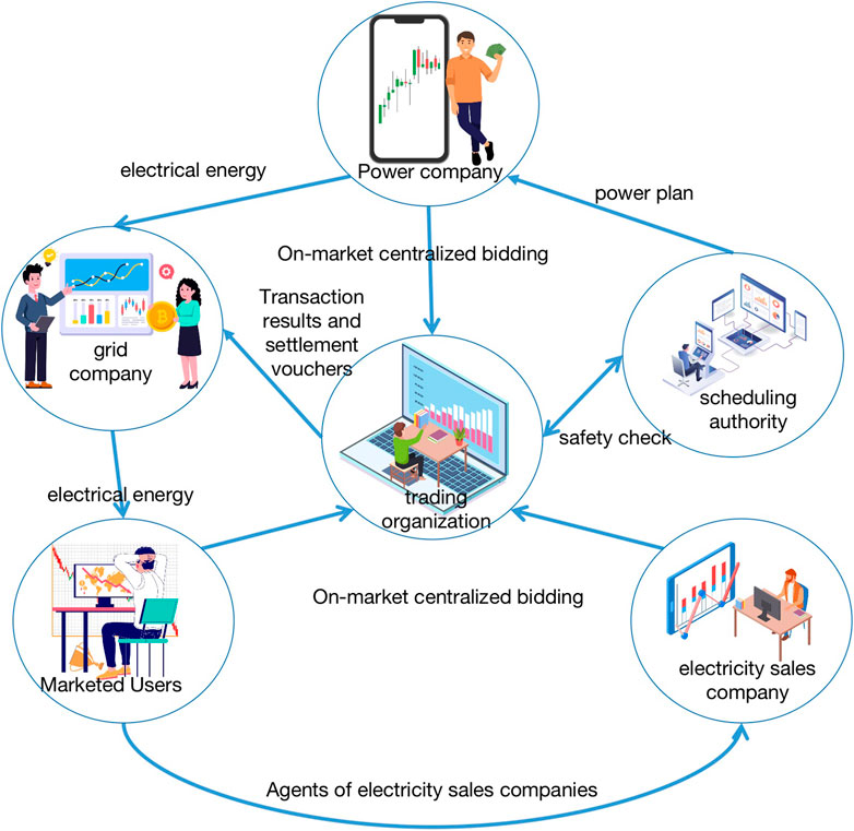
FIGURE 1. Spot market electricity price formation process.

2.2 Spearman correlation-based integrated similarity ranking of historical information

The previous section explains the formation of spot market electricity price, which is formed by the joint action of a variety of factors. This paper summarizes the research on the following existing electricity price forecasting factors: historical electricity price, market demand, thermal power output, new energy output, provincial load adjustment, and market player strategy (JI et al., 2022).

The history of electricity price, according to the electricity market before the result, is divided into the day-ahead spot price and real-time spot prices. The market demand includes the market main body, the different time scales of market demand, market demand prediction deviation, intra-provincial transactions and inter-provincial transactions, etc., between thermal power output including history and actual output of thermal power, scheduling, and modulate and participate in peak shaving, and modulate the and so on (HAN et al., 2023).

New energy output includes the historical output of new energy, forecast deviation of new energy output, and proportion of new energy output in market demand. Provincial load adjustment mainly includes medium- and long-term transaction power and inter-provincial spot transaction power (Zhang et al., 2022).

Combined with the current status of domestic and foreign electricity price forecasting research and the actual operation of China’s spot pilot, this paper selects the provincial load, thermal power output, new energy output, non-market power, and outgoing power as the correlation factors of electricity price forecasting. These correlation factors are the inputs of the electricity price forecasting model and the basis of the screening of the similarity day. In order to verify the validity of these factors selected in this paper, a province of the spot pilot was selected to run the actual operation of the electricity price forecasting model. The correlation coefficient is calculated herein. In order to verify the validity of the factors selected in this paper, the actual operating data on a province in the spot pilot are chosen as the data for factor correlation analysis, and Spearman’s correlation is used for correlation analysis. Spearman’s correlation coefficient can also be expressed in terms of rank value. Spearman’s correlation between two variables can be expressed as the Pearson correlation between the rank values of two variables. Its main formula is expressed as follows (Wu et al., 2021):

$r_s=1-\frac{6\sum d_i^2}{n\left(n^2-1\right)}.(1)$

In the equation, $d_i$ represents the rank difference between subjects, n represents the number of observations, and $r_s$ represents the correlation between two subjects.

Through the above equation, the correlations of unified scheduling load, inter-provincial demand load, new energy output, non-market output, and thermal power output are obtained: 0.8214, 0.5790, −0.7954, 0.6254, and 0.9655, respectively. It can be seen that thermal power space has the strongest correlation with the spot price, followed by the unified scheduling load, and finally, the inter-provincial demand load. In the selection of similar days, the correlation coefficient is taken as the relevant factor of weight.

2.3 FCM-based similar-day screening

The Fuzzy C-means (FCM) model is a multivariate analysis method based on partitioning. FCM is a multivariate analysis method based on division. The general steps of the algorithm can be divided into data standardization, calibration (establishing a fuzzy similarity matrix), and clustering (solving a dynamic cluster diagram matrix) and clustering (dynamic clustering map) (Cheng et al., 2022).

Data standardization: First, the dataset of correlation factors of different factors with multiple days is $U=\left\{x_1,x_2,{\dots ,x}_n\right\}$ through Spearman’s filtering, and each key correlation factor has m values constituting. Then, the original data matrix $Q$ is represented as

$Q=\left[\begin{array}{ccc}{x}_{11}& ...& x_{1m}\\ ⋮& \ddots & ⋮\\ x_{n1}& ...& x_{nm}\end{array}\right].$

In order to unify the magnitude of the data on different correlation factors, it is necessary to standardize the original data parameters, and the original factor data matrix is compressed to the interval [0,1] by using polar transform pairs.

$x_{ik}^{\prime }=\frac{x_{ik}-\underset{1\le i\le n}{\mathit{min}}\left\{x_{ik}\right\}}{\underset{1\le i\le n}{\mathit{max}}\left\{x_{ik}\right\}-\underset{1\le i\le n}{\mathit{min}}\left\{x_{ik}\right\}}\left(k=1,2,...,m\right).(2)$

Calibration (establishment of the fuzzy similarity matrix): According to the theory of the fuzzy clustering algorithm, in order to facilitate the analysis and comparison between statistical indicators, the similarity degree of two elements in the domain U is calculated as $r_{ij}=R\left(x_i,x_j\right)$. The traditional cluster analysis method of the angle cosine method of the data matrix for fuzzy processing is used to obtain the fuzzy similarity matrix R of the relevant factors. Then, the calibration model of the angle cosine method represented is as follows:

$r_{ij}=\frac{{\displaystyle {\sum }_{k=1}^m}{x}_{ik}\bullet x_{jk}}{\sqrt{{\displaystyle {\sum }_{k=1}^m}{x}_{ik}^2-{\displaystyle {\sum }_{k=1}^m}{x}_{jk}^2}}.(3)$

Clustering (seeking the dynamic clustering diagram): The fuzzy similarity matrix has self-inversion and symmetry but not necessarily transferability. In order to realize the classification of different relevant factors, it is necessary to convert the fuzzy similarity matrix R into the fuzzy equivalence matrix R*. The quadratic method is used to obtain the transfer closure t(R) of the fuzzy similarity matrix, and the transfer closure t(R) is the required fuzzy similarity matrix R*, which is t(R) = R*. For different confidence levels, λ is divided into large and small to obtain the dynamic clustering diagram of different electricity price-related factors.

In order to ensure the accuracy of similar-day screening, this paper adopts the Spearman–FCM model to screen the historical data and select the historical data that best meet the prediction demand as the base data for electricity price prediction. The specific steps are shown below:

1) A collection of factors related to electricity price factors is constructed. Then, according to the degree of influence of different factors on the electricity price, the key factors that best meet the demand for electricity price prediction are screened. This paper mainly chooses Spearman's correlation as the factor screening model.

2) According to the first step to obtain the core key factors of electricity price forecasting, further screening out the historical day and forecast day market-related factors most closely match the data. First, the different key factors are constructed to form a multi-day factor matrix, and second, the FCM model is used to cluster the different relevant factors on the forecast day and the historical day, and the clustering intervals where the different factors are located are selected.

3) According to the clustering intervals of different factors obtained in the third step, the aggregated clustered data on different factors are integrated, and the data with the highest degree of similarity obtained by clustering are sorted. Then, the data on the first 50 days are screened out as the basic data for tariff prediction.

The similar-day screening process is shown in Figure 2.

FIGURE 2

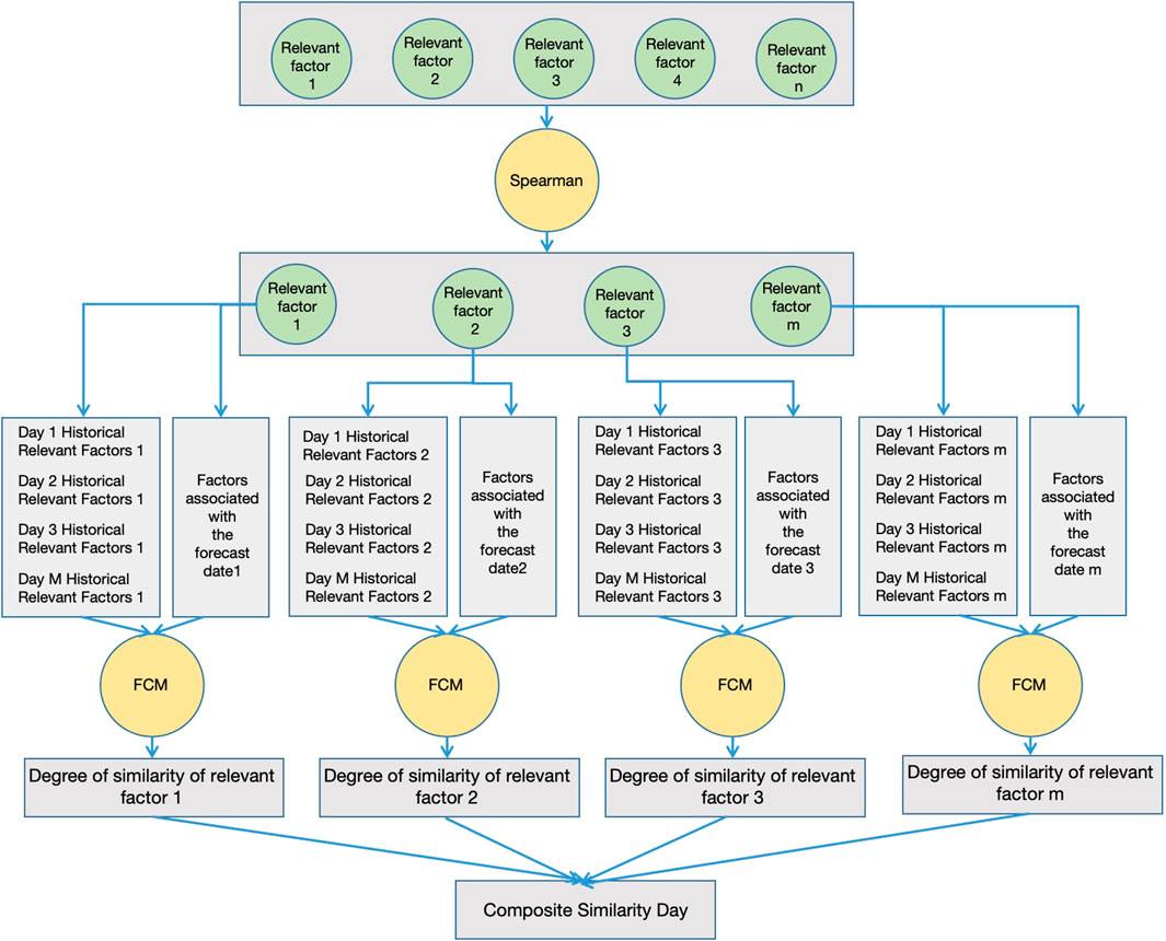
FIGURE 2. Similar day screening process.

3 Research on the multi-layer decomposition model of the electricity price sequence based on CEEMDAN-XGT

3.1 CEEMDAN model analysis

Complementary ensemble empirical mode decomposition with adaptive noise (CEEMDAN) is a signal decomposition method based on adaptive noise control further developed on the basis of CEEMD. Different from CEEMD, CEEMDAN employs an adaptive control strategy in the construction and addition of random noise in order to better control the size and distribution of the noise, thus improving the accuracy and stability of the signal decomposition (Iruela et al., 2021).

The basic process of CEEMDAN is as follows:

1) Let the original signal be $x\left(t\right)$. A normally distributed Gaussian white noise is added to obtain k times the preprocessing sequence $x_i\left(t\right)$ as in Formula (4):

$x_i\left(t\right)=x\left(t\right)+\epsilon {\delta }_i\left(t\right),i=1,2,3,...,k.(4)$

In the formula, $\epsilon$ is the noise factor and ${\delta }_i$ is the noise of the ith residual component.

2) The input sequence is decomposed using EMD to obtain the first EMD decomposed component, the mean value is taken as the decomposed signal component, and the residual component is calculated, as in Formula (5)–Formula (7):

$x_{ik}^{\prime }=\frac{x_{ik}-\underset{1\le i\le n}{\mathit{min}}\left\{x_{ik}\right\}}{\underset{1\le i\le n}{\mathit{max}}\left\{x_{ik}\right\}-\underset{1\le i\le n}{\mathit{min}}\left\{x_{ik}\right\}}\left(k=1,2,...,m\right),(5)$

$I_1\left(t\right)=\frac{1}{K}{\displaystyle \sum _{i=1}^K}{I}_1^i\left(t\right),(6)$

$r_1\left(t\right)=x\left(t\right)-I_1\left(t\right).(7)$

In the formula, $I_1\left(t\right)$ is the first signal component (IMF) after CEEMDAN decomposition; $I_1^i$(t) is the EMD decomposed signal component; and $r_1\left(t\right)$ is the residual fraction.

Similar to step 2, the jth residual component is added to the corresponding Gaussian white noise. After adding the corresponding Gaussian white noise to the jth residual component, we continue to decompose the residual signal using EMD. The decomposed signal components and residual components are shown in Formula (8) and Formula (9), respectively:

$I_j\left(t\right)=\frac{1}{K}{\displaystyle \sum _{i=1}^K}{H}_1\left(r_{j-1}\left(t\right)+{\epsilon }_{j-1}{H}_{j-1}\left({\delta }_i\left(t\right)\right)\right),(8)$

$r_j\left(t\right)=r_{j-1}\left(t\right)-I_j\left(t\right).(9)$

In the formula, $I_j\left(t\right)$ is the jth component of the CEEMDAN decomposition; $H_{j-1}$ is the EMD decomposed components; ${\epsilon }_{j-1}$ is the coefficient of noise; and $r_j\left(t\right)$ is the residual fraction.

The above steps are repeated until the extreme point is less than 2 or the artificially set number of components, and then, the decomposition is finished. At this point, the original signal is decomposed into K signal components and a residual component r(t), as in Formula (10):

$x\left(t\right)=r\left(t\right)+{\displaystyle \sum _{i=1}^K}{I}_i\left(t\right).(10)$

In the formula, $r\left(t\right)$ is the margin signal and $I_i\left(t\right)$ is the ith signal component.

After CEEMDAN decomposition, a set of IMF functions with different scales can be obtained, which have good adaptive properties and can reflect the essential characteristics of the signal at different time scales and frequencies. Compared with traditional methods such as wavelet decomposition and spectral decomposition, CEEMDAN can handle nonlinear and nonsmooth signals with better adaptability and accuracy.

3.2 XGBoost model analysis

eXtreme Gradient Boosting (XGBoost) is a machine learning library focusing on gradient boosting algorithms, developed by Tianqi Chen in February 2014 at the University of Washington. In his research, he deeply appreciated the computational speed and accuracy problems of existing libraries and built the XGBoost project for this reason (Yin et al., 2022).

Suppose we have the following objective function:

$object={\displaystyle \sum _{i=1}^n}l\left(y_i,{\widehat{y}}_i^{\left(t\right)}\right)+{\displaystyle \sum _{k=1}^t}\phi \left(f_i\right).(11)$

At each step, we add a tree to the previous step, and this new tree is added to fix the deficiencies of the previous tree. We denote the prediction at step t by y to denote

$\begin{array}{l}{\widehat{y}}_i^{\left(0\right)}=0,\\ {\widehat{y}}_i^{\left(1\right)}=f_1\left(x_i\right)={\widehat{y}}_i^{\left(0\right)}+f_1\left(x_i\right),\\ {\widehat{y}}_i^{\left(2\right)}=f_1\left(x_i\right)+f_2\left(x_i\right)+{\widehat{y}}_i^{\left(1\right)}+f_2\left(x_i\right),\\ \dots \\ {\widehat{y}}_i^{\left(t\right)}={\displaystyle \sum _{k=1}^t}{f}_k\left(x_i\right)={\widehat{y}}_i^{\left(t-1\right)}+f_t\left(x_i\right).\end{array}(12)$

For the set $M=\left\{\left.\left(x_i,y_i\right)\right\}\left(i=0,1,...,t\right)\right.$ of electricity price correlation factors after data preprocessing, where X $x_i=\left(x_0^i,x_1^i,...,x_n^i\right)$ denotes the nth dimensional feature vector of the ith sample, i.e., the n eigenvalues of the input electricity price decomposition curve, and y denotes the labeled value of the ith sample; the correlation factor M is inputted into XGBoost for training to obtain a K-tree, which can be represented as

$\begin{array}{c}{\widehat{y}}_i={\displaystyle \sum _{k=1}^K}{f}_k\left(x_i\right),f_k\in F,\\ F=\left\{f\left(x\right)=w_{q\left(x\right)}\right\},\end{array}(13)$

where ${\widehat{y}}_i$ denotes the prediction result of the ith sample; F is the base learner, i.e., the set of K-trees; $f_k$ denotes the kth regression tree; and $w_{q\left(x\right)}$ denotes the fraction of the leaf node q. The objective function during the training process is as follows:

$O={\displaystyle \sum _{i=0}^t}l\left(y_i,{\widehat{y}}_i\right)+{\displaystyle \sum _{k=1}^K}\phi \left(f_i\right),(14)$

where l is the loss function used to calculate the error between the predicted value and the true value,φ is a function that represents the complexity of the tree. The smaller the value, the lower the complexity and the stronger the generalization ability. Its expression is represented as follows:

$\phi \left(f_i\right)=\gamma N+\frac{1}{2}\mu {‖w‖}^2,(15)$

where N denotes the number of leaf nodes and w denotes the value of the node. Intuitively, the goal is to keep the prediction error as small as possible, the number of leaf nodes N as small as possible, and the value of nodes w as less extreme as possible.

By continuously optimizing in the gradient direction, the objective function becomes lower and lower because the predicted value ${\widehat{y}}_i$ can be obtained after the Tth iteration by adding the sum of the output values of the previous T-1 iterations and the value $f_T\left(x_i\right)$ of the tree structure computed in the Tth iteration so that the objective function O is converted into

$O^T={\displaystyle \sum _{i=0}^t}l\left(y_i,{\widehat{y}}_i^{\left(T-1\right)}+f_T\left(x_i\right)\right)+\phi \left(f_T\right)+C,(16)$

where C is a constant and the above equation can be optimized by a second-order Taylor expansion:

$O^T={\displaystyle \sum _{i=0}^t}\left[l\left(y_i,{\widehat{y}}_i^{\left(T-1\right)}\right)+{g_{i}f}_T\left(x_i\right))+\frac{1}{2}{h}_i{f_T}^2\left(x_i\right)\right]+\phi \left(f_T\right),(17)$

where $g_i={\partial }_{\widehat{y}\left(T-1\right)}l\left({\mathrm{y}}_{\mathrm{i}},{\widehat{\mathrm{y}}}_{\mathrm{i}}^{\left(\mathrm{T}-1\right)}\right)$ is the first-order derivative of the prediction error with respect to the current model and ${\text{h}}_{\text{i}}={\partial }_{\widehat{\text{y}}{\left(\text{T}-1\right)}^2}\text{l}\left({\text{y}}_{\text{i}},{\widehat{\text{y}}}_{\text{i}}^{\left(\text{T}-1\right)}\right)$ is the second-order derivative of many prediction errors with respect to the current model.

Since the residuals of the model at T-1 are known at the Tth iteration, the objective function is converted into the form of leaf-node accumulation by removing the constant term $\text{l}({\text{y}}_{\text{i}},{\widehat{\text{y}}}_{\text{i}}^{\left(\text{T}-1\right)}$ and expanding the above equation as follows:

$O^T={\displaystyle \sum _{j=1}^N}\left[G{w}_j+\frac{1}{2}\left(H+\mu \right)w_j^2\right]+\gamma N,(18)$

$G={\displaystyle \sum _{i\in I}}{g}_i,(19)$

$H={\displaystyle \sum _{i\in I}}{h}_i,(20)$

where I denotes the set of samples on each leaf node, $I_j=\left\{i|q\left(x_i\right)=j\right\}$, $q\left(x_i\right)$ is the tree structure function, $w_j$ denotes the output of each leaf node of the tree fraction, N denotes the number of leaf nodes in the split tree, and γ is the weight factor, which are used to control the weights of the corresponding parts.

After creating the boosted decision tree, the feature importance of each feature is obtained by calculating the gain. Similar to the information gain and Gini index in decision trees, the XGBoost algorithm adds a gain to the existing leaves at each attempt. The XGBoost algorithm calculates the gain of selected features every time it tries to add a partition to an existing leaf. The XGBoost algorithm calculates the gain of the selected feature every time it tries to add segmentation to an existing leaf.

$Gain=\frac{1}{2}\left[\frac{G_L^2}{H_L+\partial }+\frac{G_R^2}{H_R+\partial }+\frac{{\left(G_L+G_R\right)}^2}{H_L+H_R+\partial }\right]-\gamma ,(21)$

where the subscripts L and R denote the left and right subtrees, respectively; $\frac{G_L^2}{H_L+\partial }$ denotes the left subtree score; $\frac{G_R^2}{H_R+\partial }$ denotes the right subtree score; and $\frac{{\left(G_L+G_R\right)}^2}{H_L+H_R+\partial }$ denotes the score of the current node that is not split.

The importance of a feature is calculated in a single boosted tree by the gain of each feature split point; the larger the gain, the larger the weight. The more lifting trees a feature is selected from, the more important the feature is. Finally, the results of a feature in all the boost trees are weighted and averaged to obtain the importance score. After sorting the features in the descending order of importance score, m (m < n) important features affecting electricity price are filtered out by setting different thresholds.

3.3 Construction of the CEEMDAN-XGT tariff decomposition model

Since the spot market is a short-term market, the spot market price shows strong volatility, and this volatility is mainly due to the rapid change in market information. At the same time, this large volatility will affect the accuracy of the electricity price prediction, so this paper adopts the CEEMDAN-XGT model to decompose the similar-day dataset to obtain the historical data that can reflect the characteristics of the electricity price so as to provide the accuracy of the prediction model, and the specific steps are as follows:

1) The historical electricity prices in the similar-day data are decomposed using CEEMDAN to form multiple decomposition curves, which represent the trend of electricity prices;

2) The different decomposition curves obtained through step 1 can reduce the error of electricity price prediction to a certain extent, but different decomposition curves have different structures of influencing factor composition. So, for different decomposition sequences, the XGT model is used to screen to obtain the most consistent with the requirements of each decomposition curve factor ranking as the input for the next step of prediction.

3) Different decomposition curves of electricity price and the corresponding factor relationships are brought into the prediction model, which can reduce the influence of electricity price volatility on the prediction model error and also find the degree of influence of different factors on different days.

The electricity price curve decomposition process is shown in Figure 3.

FIGURE 3

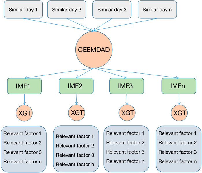
FIGURE 3. Electricity price curve decomposition process.

4 Construction of the MPA-CNN-BiLSTM electricity price prediction model considering market information volatility

4.1 Marine predators optimization algorithm

The marine predators algorithm (MPA) is a new meta-heuristic optimization algorithm proposed by Afshin Faramarzi et al. in 2020. MPA optimization is divided into three stages: the initialization stage, optimization stage, and fish aggregation device (FAD) effect or eddy current stage [28]. The specific MPA optimization process can be described as follows:

1) Initialization phase: The algorithm parameters are set to initialize the location of the prey within the search scope. It can be described as

$X_0=X_{\mathit{min}}+rand\left(X_{\mathit{max}}-X_{\mathit{min}}\right).(22)$

In Formula (22), $X_{\mathit{max}}$ and $X_{\mathit{min}}$ denote the search space of the prey and rand() is a random number within [0,1].

2) Optimization stage: The optimization phase is divided into early iteration, middle iteration, and late iteration. At the beginning of the iteration, the current iterations are less than 1/3 of the maximum iterations. Predators are faster than their prey and updating prey through Brownian random movement.

$\left\{\begin{array}{l}{stepsice}_i=R_B\otimes \left({Elite}_i-R_B\otimes {prey}_i\right)\\ {prey}_i={prey}_i+P{\bullet R}_B\otimes {stepsice}_i\end{array}\right.Iter<\frac{1}{3}\max \_Iter.(23)$

In Formula (23), $stepsice$ is the step size, $R_B$ is the Brownian random walk vector with normal distribution, ${prey}_i$ is the prey matrix with the same dimension as the static matrix, ${Elite}_i$ is the elitist matrix constructed by the top predator, $\otimes$ is a multiplicative operation item by item, P equals 0.5, and R is a [0,1] uniform random vector. N is the population size, and $Iter$ and $\text{max\hspace{0.17em}}\_\text{Iter}$ represent the current and maximum iterations, respectively.

In the middle of an iteration, the current iteration is less than 2/3 of the maximum. The population is divided into two parts, in which the prey does the levy movement and is responsible for the algorithm development in the search space. Predators perform Brownian motion, responsible for the algorithm to explore in the search space, and gradually develop from exploration to a development strategy.

At the end of the iteration, the current iteration number is more than 2/3 of the maximum iteration number. In particular, to improve the local development, the predator is slower than the prey, and predator roaming is based on the Levy distributed random vector.

$\left\{\begin{array}{l}{stepsice}_i=R_L\otimes \left({R_L\otimes Elite}_i-{prey}_i\right)\\ {prey}_i={Elite}_i+P\bullet CF\otimes {stepsice}_i\end{array}\right.Iter>\frac{2}{3}\max \_Iter.(24)$

In the above equation, $R_L$ is the Levy distributed random vector and $\text{CF}={\left(1-\text{Iter}/\text{max}\_\text{Iter}\right)}^{2\text{Iter}/\text{max}\_\text{Iter}}$ is the adaptive parameter controlling predator movement compensation.

3) FAD effect or eddy current: Fish aggregation devices (FADs) or vortex effects often change the behavior of marine predators, which enables the MPA to overcome the premature convergence problem and adjust the local extremum.

${prey}_i=\left\{\begin{array}{c}{prey}_i+CF\left[X_{\mathit{min}}+R_L\otimes \left(X_{\mathit{max}}-X_{\mathit{min}}\right)\right]\otimes U,r\le FADs,\\ {prey}_i+\left[FADs\left(1-r\right)+r\right]\left({prey}_{r1}-{prey}_{r2}\right),r>FADs.\end{array}\right.(25)$

In Formula (25), $FAD$ is the influence probability, which is 0.2; $U$ is the binary vector; $r$ is the random number in [0,1]; and $r1$ and $r2$ are the random indexes of the prey matrix.

4.2 Principles of convolutional neural network modeling

A convolutional neural network (CNN) consists of five parts, namely, the input layer, convolutional layer, pooling layer, fully connected layer, and output layer, in which the alternation of the convolutional layer and pooling layer can better extract the local characteristics of the data and reduce the feature dimensions; the sharing of weights not only reduces the number of weights but also the complexity of the model [29]. The formula of convolution is

$V_j^l=\delta \left({\displaystyle \sum _{S\in M_j}}{V}_s^{l-1}\bullet K_{sj}^l+b_j^l\right),(26)$

where the prescribed input layer is layer $l-1$, $V_s^{l-1}$ denotes the sth feature of the input layer, the output layer is layer l, $V_j^l$ denotes the jth feature of the output layer, $K_{sj}^l$ denotes the elements of the convolution kernel, $b_j^l$ is the bias term, and σ is the activation function.

4.3 Principles of BiLSTM modeling

LSTM has special memory and forgetting patterns; thus, flexibly adapting to the basic cell structure of the LSTM network includes input gates, output gates, and forgetting gates.

The specific formula is as follows:

$i_t=\rho \left(W_{ix}{x}_t+W_{ih}{h}_{t-1}+b_i\right),(27)$

$f_t=\rho \left(W_{fx}{x}_t+W_{fh}{h}_{t-1}+b_f\right),(28)$

$g_t=\phi \left(W_{gx}{x}_t+W_{gh}{h}_{t-1}+b_g\right),(29)$

$o_t=\rho \left(W_{ox}{x}_t+W_{oh}{h}_{t-1}+b_o\right),(30)$

$C_t=g_t\otimes i_t+C_{t-1}\otimes f_t,(31)$

$h_t=\phi C_t\otimes o_t,(32)$

where $i_t$, $f_t$, and $o_t$ are states of input gates, oblivion gates, and output gates, respectively; $g_t$, $C_t$, and $h_t$ are states of input nodes, state units, and intermediate outputs, respectively; $\rho$ is the sigmoid function; $\phi$ is the tanh function; $W$ is the corresponding gate weights; $b_i$, $b_f$, $b_g$, and $b_o$ are the corresponding biases of the corresponding gates; and $\otimes$ is the element-by-element multiplication.

The structure of BiLSTM is shown in Figure 4, which consists of two LSTM networks in the forward and reverse directions, and can utilize the before-and-after change rule of the data to make a bi-directional prediction. BiLSTM has more advantages than LSTM for the information feature extraction of the complex power data in the spot tariff prediction, and it has not increased the requirements for the amount of data. Therefore, using BiLSTM for electricity price prediction can improve the model prediction accuracy.

FIGURE 4

FIGURE 4. Structure of BiLSTM algorithm.

4.4 Constructing an MPA–CNN–BiLSTM electricity price prediction model for market information volatility

The generation of electricity price in the spot electricity market has a large uncertainty and contains a large amount of uncertainty information, which leads to a lot of parameters affecting the prediction accuracy of the prediction model. Therefore, the prediction of electricity price for the spot electricity market cannot rely on a single model and requires an effective data processing method and a scientific combination of the model, which identifies the interplay of factors, reduces the error, and improves the prediction accuracy.

Therefore, this paper adopts a three-stage structure to construct the electricity price prediction model for the spot electricity market based on the consideration of the volatility of market information. The first stage is optimizing the original data and extracting similar-day information. The FCM–Spearman method is mainly used to classify and evaluate the original dataset and the relevant factor information on the forecast day, and select the days with the highest trend of change in the relevant information on the forecast day as the training set of the forecast day; the second section improves the interaction characteristics between the relevant factors and the electricity price, and reduces the impact of the stronger volatility of the electricity price on the prediction of the electricity price. In this part, CEEMDAD is mainly used to decompose the original electricity price data, and the volatility of the original electricity price data is hierarchically divided into sequences. Then, the XGT model is used to match the different decomposition sequences with the relevant factors, and the factor with the closest influence of each relevant factor is selected as the data input for the next segment. In the third segment, the data on different segments in the second segment are inputted into the MPA–CNN–BiLSTM model, which can realize the complementary characteristics of the model and achieve the effect of error reduction compared with the traditional single model, and at the same time, optimization using the MPA algorithm can realize the rationalized configuration of the model parameters.

The first two breaks of this paper were elaborated in the previous sections, and this section further analyzes the process of MPA–CNN–BiLSTM. When the electricity price prediction is carried out, the BiLSTM model will be trained by extracting the local features from the CNN, which can make the two models complement each other and obtain better prediction results. The CNN–BiLSTM model is optimized by the MPA algorithm, and then, the CNN–BiLSTM model is constructed for electricity price prediction. The CNN model consists of two convolutional layers and two maximum pooling layers, and the ReLU function is used as the activation function.

The MPA–CNN–BiLSTM algorithm flow is shown below:

Step 1. The decomposition data on similar days are divided into a training set and test set and performed dimensionless.

Step 2. The model with the number of hidden layer units, the learning rate, and the convolution kernel in the model is initialized as the optimization object, and the MPA is initialized.

Step 3. The fitness of the model is calculated based on the local optimum and the dissuasion optimum of the MPA algorithm, and the mean square error (MSE) is selected as the evaluation criterion.

Step 4. The MPA is iteratively updated using formula (23) to calculate the latest optimized position.

Step 5. When the iteration is completed or the optimal position is searched, then the termination condition is satisfied, and the optimal hyperparameters are obtained. If it is not satisfied, step 3 is repeated to iterate again.

Step 6. A CNN–BiLSTM model is constructed using the optimal hyperparameters.

Step 7. The CNN performed feature extraction of the electricity price.

Step 8. The processed data are input into the BiLSTM model, and model training is performed to output the final prediction results.

In this paper, in order to verify the effectiveness of the model, the performance of the electricity price prediction model using the root mean-square error (RMSE), mean absolute percentage error (MAPE), mean absolute error (MAE), and $R^2$. The formula for the specific effectiveness evaluation index is shown below:

$E_{RMSE}=\sqrt{\frac{1}{n}{\displaystyle \sum _{i=1}^n}{\left(P_i-p_i\right)}^2},(33)$

$E_{MAPE}=\frac{1}{n}{\displaystyle \sum _{i=1}^n}\frac{\left|P_i-p_i\right|}{P_Z}\times 100\%,(34)$

$E_{MAE}=\frac{1}{n}{\displaystyle \sum _{i=1}^n}\left|P_i-p_i\right|,(35)$

$R^2=\frac{{\displaystyle {\sum }_{i=1}^n}{\left(P_i-{\overline{p}}_i\right)}^2}{{\displaystyle {\sum }_{i=1}^n}{\left(p_i-{\overline{p}}_i\right)}^2}.(36)$

The specific flow of the electricity price prediction model proposed in this paper considering market information is shown in Figure 5.

FIGURE 5

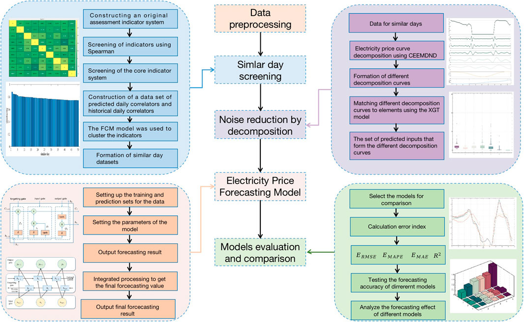
FIGURE 5. Spot market electricity price forecasting modelling process.

5 Simulation analysis

5.1 Scenario description

According to the characteristics of electricity price formation in the spot electricity market, this paper proposes an electricity price forecasting model considering market volatility. In order to verify the validity of the model proposed in this paper, the operation data on a provincial spot pilot in China are used. Compared with the construction of a foreign electricity market, the diversity of China’s electricity market is more representative. Therefore, the data on China’s spot pilot can not only reflect the operation characteristics of China’s electricity market but also meet the business needs of different electricity market players in our country, which is of practical significance. Some of the data are shown in Figure 6.

FIGURE 6

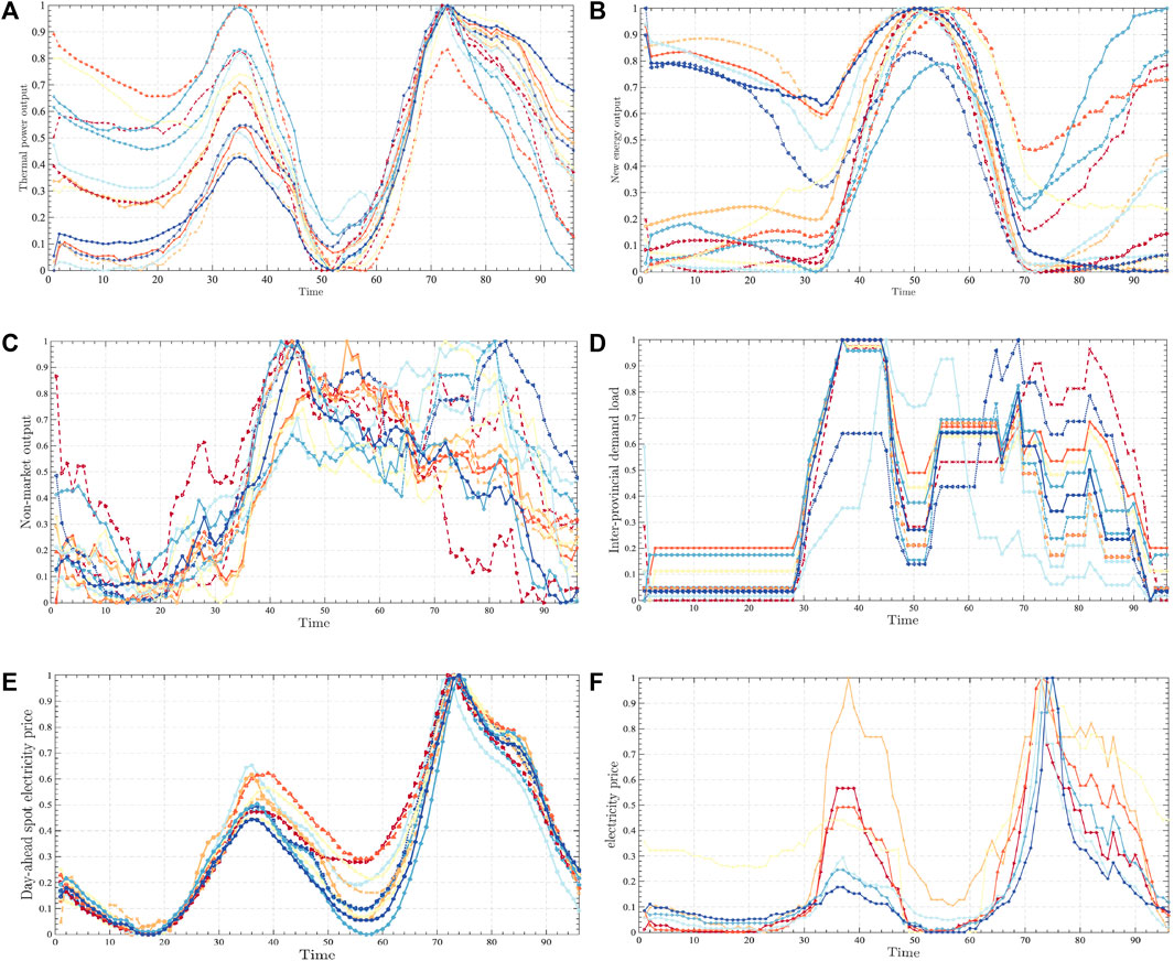
FIGURE 6. Basic scenarios.

The above is part of the original dataset selected for this paper, mainly the selected thermal power output, new energy output, non-market output, outgoing power, and provincial load data. In order to further show the relevance of these data and the market price trend, this paper intercepts the simultaneous electricity price trend data, as shown in Figure 6F.

In order to implement the model proposed in this paper, MATLAB 2020B is used as the implementation tool, and the computer uses Windows 10, running memory 16 GB, and a hard disk capacity of 2 TB.

5.2 Electricity price prediction model implementation

The dataset selected in this paper is the day-ahead electricity price data on a provincial spot pilot from 1 January 2022 to 31 May 2023. The time granularity of the electricity price is 15-min nodes, i.e., 96 points per day. At the same time, in order to show that the model proposed in this paper can achieve effective electricity price forecasting and apply it to practical work, 31 May 2023 is selected as the forecasting day for comparative analysis. According to the model process mentioned above, the steps of similar-day screening, electricity price sequence decomposition, and electricity price forecasting are carried out to form a complete electricity price forecasting validity verification. The forecast day market information is shown in Figure 7.

FIGURE 7

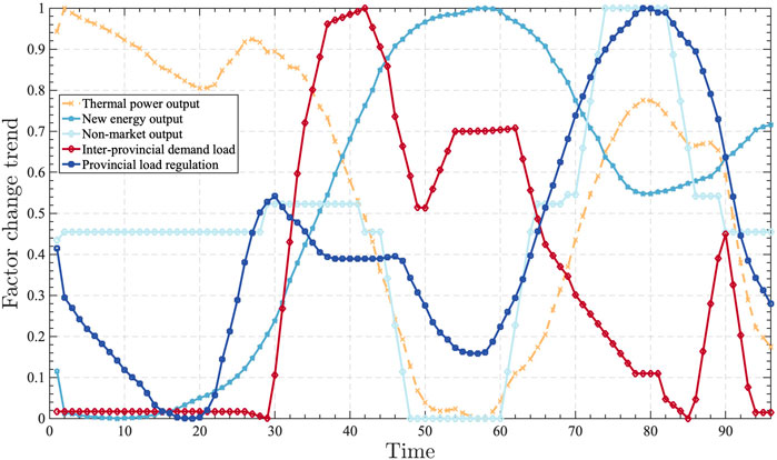
FIGURE 7. Forecast day market information.

Electricity price forecasting is a comprehensive technology, which includes computer information processing technology, and information technology emphasizes that correct input can produce correct output. Therefore, electricity price forecasting needs to ensure the accuracy of the data. In order to achieve this goal, it is necessary to screen out the historical days with similar market conditions as the basic data. This is the role of similar-day screening. This paper chooses Spearman–FCM as the similar-day screening model.

In the previous section, the Spearman model was used to screen out the relevant factors, which will not be repeated here. The focus is to use the FCM model to find the most similar dates of different related factors for the selected related factors. The specific screening diagram is shown in Figure 8.

FIGURE 8

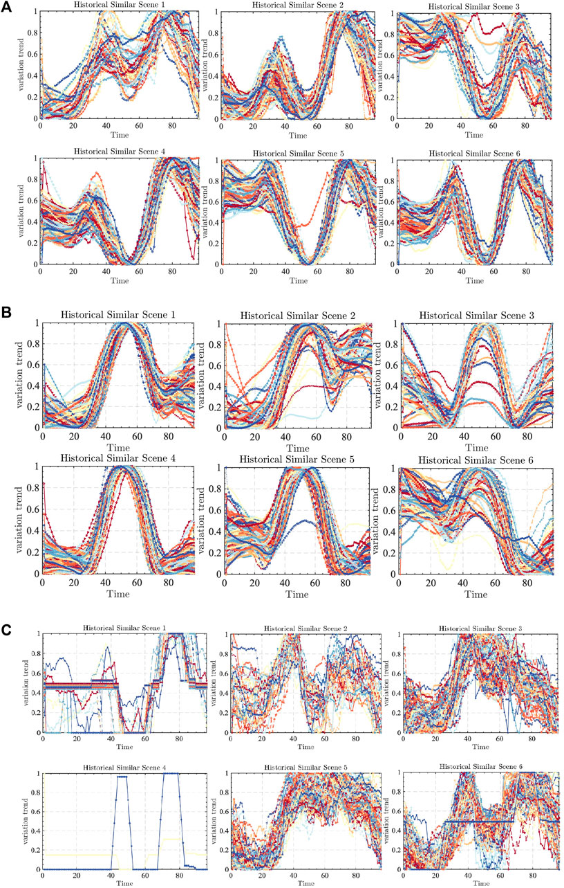
FIGURE 8. The specific screening diagram.

Figure 8A shows that the running FCM model divides the forecast day into historical similar day scenario 1. The thermal power output in the historical similar day scenario presents two peaks compared with other scenarios, but compared with the sixth scenario, the trough runs higher, indicating that the day’s new energy is still unable to meet the needs of the market during the period of large-scale development, and thermal power is needed to ensure the operation of the market. At the same time, according to the scene classification of historical similar days, there are 186 days of data that can meet the similar scenes of the forecast day. These data will be used as the basic data source for comprehensive discrimination.

According to Figure 8B, the new energy output of the forecast day is divided into historical similar scene 1. The new energy output of the historical similar scene conforms to the general characteristics of the new energy output. Historical similar scene 1 and historical similar scene 5 have the opposite operation trend. Scene 1 is less in the early morning and more in the evening. Scene 5 is the opposite. This is mainly due to seasonal differences. Historically similar scenario 3 combines the changing trends of scenarios 1 and 5. In a historically similar scenario 1, there are 157 historically similar days as alternatives.

According to the above Figure 8C, the non-market output shows a lot of uncertainty. This part of the electricity is mainly caused by the instability of the system. The division of the forecast day is mainly concentrated in the similar day scenario 1, with a total of 213 days of similar output.

Figure 9A shows that there is some similarity in the historical similarity scenarios 1, 2, and 3, with lower demand during the early morning hours and higher during the midday hours. However, there are many differences in the trends of the three scenarios in the peak period, which leads to the inconsistency in the market’s supply and demand. The judgment of the similarity of outgoing power needs to be combined with the supply and demand of the outer provinces, and outgoing power on the forecast day is classified into similarity scenario 1, and there are a total of 151 days.

FIGURE 9

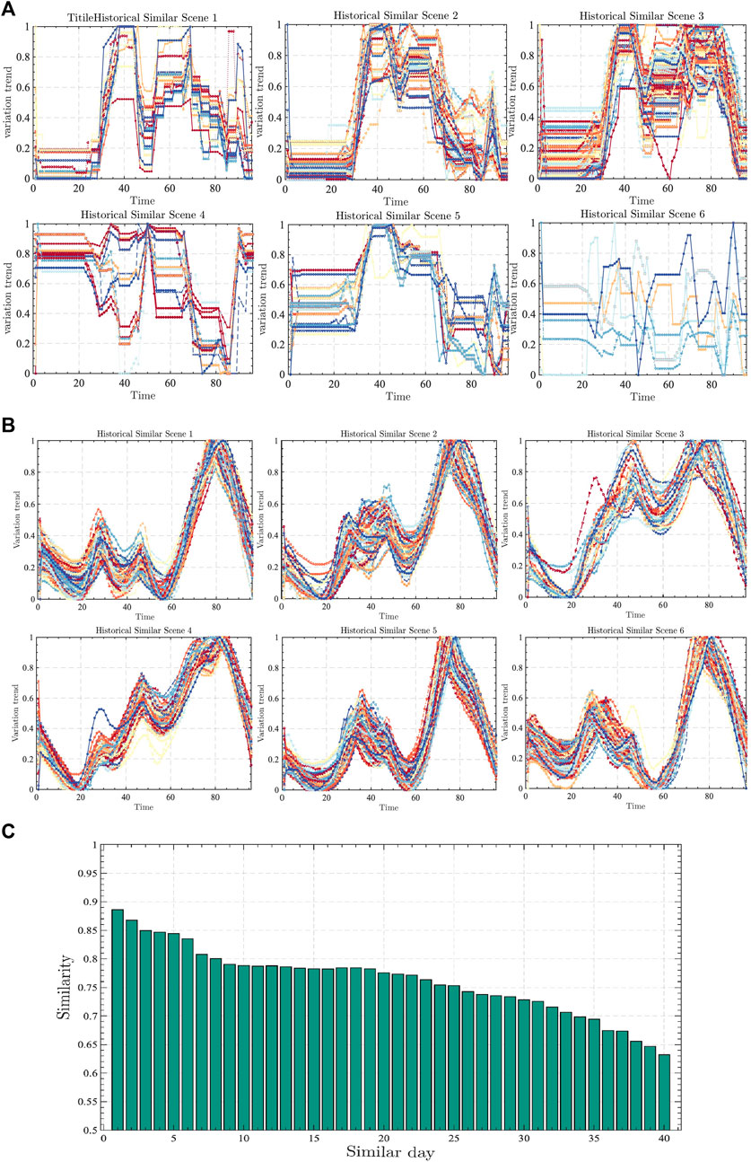
FIGURE 9. Similar day screening.

Figure 9B shows that the provincial load has a certain degree of regularity, and the trend of fluctuation has a certain degree of similarity. The main difference is that the local volatility is different; the number of peaks presented and the location of the inconsistency, which indicates that the corresponding provincial load is stable as a whole, and the forecasting day of this paper are classified into the historical similarity day scenario 2, with a total of 82 similarity days.

Through the clustering of various factors above, the historical similarity days of different factors are formed, and these similarity days can only represent the degree of similarity of the respective factors in the history, while the electricity price is the result of the integrated effect. So, it is necessary to further sort out the historical similarity days of various related factors to form the integrated historical similarity days as the data source of electricity price prediction. The specific steps are shown as follows.

The same dates of different historical similarity days are screened out to form a comprehensive historical similarity day dataset; this is because only the historical information about the same day can have a direct impact on the electricity price on that day. The above results show that the total number of historical similarity days of thermal power is 186, the total number of historical similarity days of new energy is 157, the total number of historical similarity days of non-marketed output is 213, the total number of similar days of external transmission load is 151, and the total number of similar days in history of provincial load is 82.

These similar days in history are extracted from the original data source, and the total number of days that meet the requirements is 65. Second, the integrated historical similar-day dataset of 65 days is sorted according to the degree of deviation of different factors, and the smaller the deviation, the higher degree of similarity, which is mainly calculated as

$Z_i=1-\frac{{\displaystyle {\sum }_i^{65}}{\displaystyle {\sum }_j^5}\left(y^j-x_i^j\right)-\mathit{min}{\displaystyle {\sum }_i^{65}}{\displaystyle {\sum }_j^5}\left(y^j-x_i^j\right)}{\mathit{max}{\displaystyle {\sum }_i^{65}}{\displaystyle {\sum }_j^5}\left(y^j-x_i^j\right)-\mathit{min}{\displaystyle {\sum }_i^{65}}{\displaystyle {\sum }_j^5}\left(y^j-x_i^j\right)}.(37)$

In the above equation, $Z_i$ denotes the degree of composite similarity of the historical day, $y^j$ denotes the correlation factor of the jth similarity factor of the prediction day, and $x_i^j$ denotes the jth similarity factor of the historical composite similarity day of the ith day. The higher the degree of composite similarity, the higher the adoption of information on that day. The specific consolidated ranking results are shown in Table 1.

TABLE 1

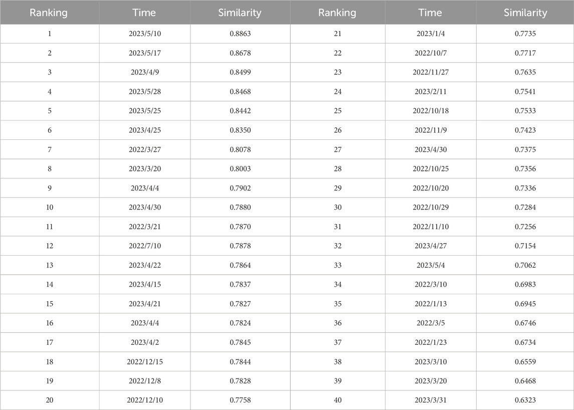
TABLE 1. Similarity and ranking of similar days.

The following conclusions can be obtained through the similar-day screening model: a) the Spearman model shows that the two factors that have a greater impact on the price of electricity are thermal power and new energy, which is mainly due to the fact that, at present, the largest market subject is still thermal power, and second, the new energy belongs to the full consumption, so it has a greater impact on the price of electricity; b) the province’s thermal power outlets, new energy outlets, and the provincial loads have a certain degree of regularity, which indicates that the market is relatively stable, and the installed capacity of new energy has no changes, which is in line with the current status quo of the province’s current development of the electricity market. The sorting of similar days is shown in Figure 9C.

In this paper, 40 days of historical days with a high similarity are screened according to the similar-day screening model, and these data are used as inputs to the CEEMDAD–XGT–MPA–CNN–BiLSTM model. Among them, CEEMDAD–XGT, as the second stage of tariff prediction, decomposes the raw tariff data, and then uses XGT to screen the different decomposition curves for their respective correlations, which is described in detail in the next part of this paper.

In this paper, there are a total of 40 days of historical electricity price as the main sequence and five related factors as the secondary sequence of input, but the volatility of the original electricity price is large and will affect the impact of the learning ability of the prediction model. So, decomposition–refactoring reduces the impact of volatility on the prediction model but retains the trend of changes in the original sequence, so this paper chooses the CEEMDAD decomposition. Part of the decomposition curve is shown in Figure 10.

FIGURE 10

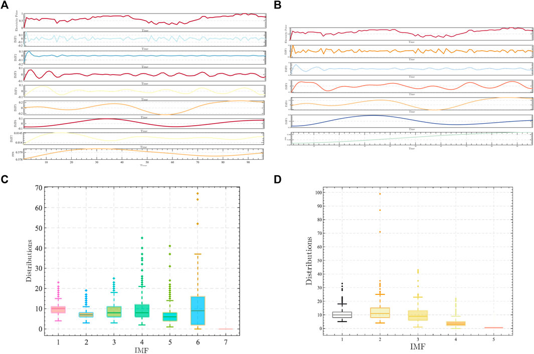
FIGURE 10. Comparison of results from different tariff decomposition models.

Figures 10A,B show the curves of CEEMDAD and EEMD of the same-day electricity price, respectively. The above results show that the number of IMFs of the two kinds of decomposition is different, indicating that the gradual decomposition of the electricity price curve is different. Compared with the traditional model, the IMF sequence obtained by the CEEMDAD model selected in this paper is more and more detailed. At the same time, the final reintegration of the data is relative to the EEMD of the bias of the reduction of the data is applied to ensure that the original sequence of the characteristics of the original sequence.

Figure 10C represents the box plot of the number of internal envelope iterations for CEEMDAD; Figure 10D represents the box plot of the number of internal envelope iterations for EEMD. The box plots represent the minimum, lower quartile, median, upper quartile, and maximum values of different IMF iterations. CEEMDAD decomposes a total of seven IMFs and one RES, and EEMD decomposes a total of five IMFs and one RES. The box plot distributions of the initial decomposition curves and the final decomposition curves of the two decompositions have the same integral, but the intermediate several decomposition curves are very different, which is mainly caused by the different processing abilities for noise.

The above results show that the CEEMDAD used in this paper is more explicit than the traditional EEMD of the tariff curve. The error of the decomposition reconstructed curve is relatively small, and the number of iterations of each decomposition curve is relatively stable. Since XGT mainly extracts the relevant factors from the main sequence to match different curves, the role of the relevant factors is similar to that of the Spearman model in the previous section. Next, this paper predicts the different decomposition curves to form the final electricity price prediction results.

According to the previous description, this paper takes 40 days of similar-day data as the basic data for tariff prediction, and decomposes these 40 days of tariff data using the CEEMDAD model and matches different factors to decompose the curves one by one using the XGT model to form different combinations of model inputs, forming a multi-input model. The third stage of the tariff prediction model adopts the MPA–CNN–BiLSTM model. The model MPA belongs to the heuristic algorithm. In order to ensure the reasonableness of the optimization algorithm, this paper sets the basic parameters of the MPA model to the maximum number of iterations, 1,000, the number of search groups is set to 50, and the FADs are set to 0.3. In addition, in order to verify the effectiveness of the model proposed in this paper, the number of the EEMD–MPA–CNN–BiLSTM, CNN–BiLSTM, BiLSTM, LSTM, and other models is increased for comparative analysis.

Figure 11 shows that the model proposed in this paper predicts the trend of electricity price, and the actual electricity price is basically consistent, which, to a certain extent, is in line with the needs of the power market players to make trading decisions. At the same time, Figure 11 shows that the absolute error of the model proposed in this paper is relatively low, especially in the morning and evening hours, and the main error is distributed in the midday hours, which is mainly due to the midday hours being subjected to the new energy output uncertainties. This is mainly due to the uncertainty of the new energy output in the noon time, so the model proposed in this paper has certain applicability.

FIGURE 11

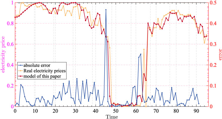
FIGURE 11. CEEMDAD-MPA-CNN-BiLSTM electricity price forecast curve.

5.3 Analysis of model validity

In order to better verify the validity of the model proposed in this paper, different models are used for comparison, i.e., EEMD–MPA–CNN–BiLSTM, CNN–BiLSTM, BiLSTM, and LSTM. On one hand, it is verified that the decomposition proposed in this paper is superior to the traditional decomposition, and on the other hand, it is verified that the prediction model proposed in this paper is superior to the traditional model of the same series. The prediction results of these models are shown in Figure 12.

FIGURE 12

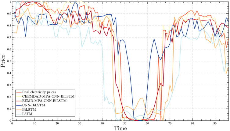
FIGURE 12. Comparison of prediction effects of different prediction models.

Figure 12 shows that the model proposed in this paper is closer to the real electricity price curve than the other models, especially in the evening and night, followed by the EEMD–MPA–CNN–BiLSTM model prediction results. The predicted curves are slightly worse than those of the model proposed in this paper but better than those of the CNN–BiLSTM, BiLSTM, and LSTM models, which indicates that the structure of the prediction model proposed in this paper is effective and can meet the needs of the electric price forecasting. However, the prediction results of the noon hour are slightly in error compared with those of the other hours, which is mainly due to the increase of output of new energy at noon, which leads to the increase of load uncertainty. In order to further illustrate the advantages of the model proposed in this paper, the prediction results of different models are next fitted with the actual results to verify the validity, and the specific results are shown in Figure 13.

FIGURE 13

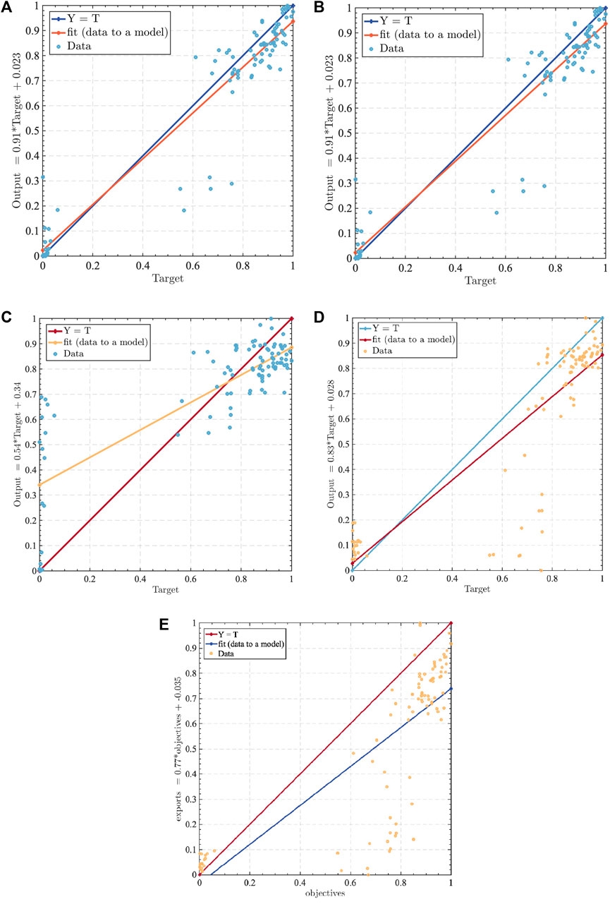
FIGURE 13. Prediction bias of different prediction models.

The fitting results given in Figure 13 show that the model proposed in this paper has the highest fit, followed by EEMD–MPA–CNN–BiLSTM, which indicates that the model chosen in this paper, as well as the structure of the constructed tariff prediction model, is more reasonable and can meet the needs of tariff prediction, and at the same time, Figure 13 shows that the basic model adopted in this paper, BiLSTM, also has a certain prediction advantage, which indicates that the model in this paper meets the basic needs of electricity price prediction. From this, we obtain the order of the prediction result advantage as follows: CEEMDAD–MPA–CNN–BiLSTM > EEMD–MPA–CNN–BiLSTM > CNN–BiLSTM > BiLSTM > LSTM.

To better illustrate the advantages of the model proposed in this paper, SSE, MSE, RMSE, and R² are used to verify that the error of the proposed prediction model is low. The errors of the prediction model in this paper are all lower than those of the other four prediction models. Compared with the model of EEMD decomposition, SSE is reduced by 0.6706 and MSE is reduced by 0.007, which indicates that the prediction error of this model is lower and can provide price reference for market players. The specific error results are shown in Table 2.

TABLE 2

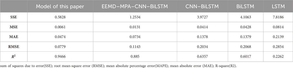
TABLE 2. Different model errors.

Table 2 shows that the model errors of this paper are all the lowest, and the results of R² are better among the five models, which shows that the model of this paper has a certain degree of sophistication. At the same time, combined with the prediction curves of different models in the previous section, the following conclusions can be obtained: first, China’s electricity market is still in the development stage, resulting in the existence of great volatility in electricity prices, and the historical market scenario is more dispersed, which leads to the fact that there is still a certain amount of error in the prediction of electricity prices, and second, all the current models present a high level of error at the midday hours, which is mainly due to the fact that China still prioritizes the consumption of new energy. The new energy output at noon has a great impact on the electricity price, so we should focus on the development of new energy in the future. Third, the evening peak price of electricity is calibrated by several models, and future market players can focus on the trend of electricity prices during these hours.

6 Conclusion

In this paper, a similar daily screening model is proposed based on the improved Spearman–FCM model by analyzing the relevant factors of the spot market and further screening the raw data to ensure the reasonableness of the forecast data. By introducing CNN–BiLSTM and MPA models, the Spearman–FCM–CEEMDAD–MPA–CNN–BiLSTM model is constructed on the basis of considering the components of CNN–BiLSTM. The model is validated by spot electricity price proposed previously, and the prediction results of five models, including EEMD–MPA–CNN–BiLSTM, CNN–BiLSTM, BiLSTM, and LSTM, are compared, and the following conclusions are drawn.

Screening the raw data using the Spearman–FCM model to obtain the number of historical days similar to the market scenario on the prediction date can optimize the raw data structure, ensure the accuracy of the input data on the prediction model, reduce the generalization ability of the strengthened prediction model, and improve the prediction accuracy of the prediction model.

Combined with the relevant data on the spot market, the five models are predicted, and it is verified that Spearman–FCM–CEEMDAD–MPA–CNN–BiLSTM can handle the peak tariffs better than the other models, realizing the requirement of the full-cycle prediction, and avoiding the prediction problem of a single model that can only deal with the less volatility.

Both the proposed model and the validation model in this paper have errors, and the errors are concentrated in the outliers of the market electricity price, which indicates that in the process of electricity price prediction, not only should the public information released by the market trading institutions be taken into account but also the behavioral characteristics of the market players. The factors such as the power system security scheduling should also be considered, which will affect the trend of the market electricity price.

At present, China’s spot market is in the primary stage of construction, the trend of electricity prices is not stable, and there will be the problem of electricity price adjustment. Therefore, in the process of electricity price forecasting, corrections should be made according to market characteristics.

Data availability statement

The original contributions presented in the study are included in the article/Supplementary Material; further inquiries can be directed to the corresponding author.

Author contributions

QL: conceptualization, project administration, supervision, validation, and writing–original draft. WC: conceptualization, formal analysis, software, validation, and writing–original draft. XZ: investigation, methodology, software, validation, and writing–review and editing. SZ: data curation and writing–original draft. XG: writing–review and editing. BZ: resources and writing–original draft.

Funding

The author(s) declare that no financial support was received for the research, authorship, and/or publication of this article.

Conflict of interest

Authors QL and WC were employed by China Southern Power Grid Co., Ltd. Author SZ was employed by Guangdong Power Gird Corporation. Author XG was employed by Guangdong Power Trading Center Co., Ltd. Author BZ was employed by Beijing QU Creative Technology Co., Ltd.

The remaining author declares that the research was conducted in the absence of any commercial or financial relationships that could be construed as a potential conflict of interest.

Publisher’s note

All claims expressed in this article are solely those of the authors and do not necessarily represent those of their affiliated organizations, or those of the publisher, the editors, and the reviewers. Any product that may be evaluated in this article, or claim that may be made by its manufacturer, is not guaranteed or endorsed by the publisher.

References

Beltrán, S., Castro Airizar, I., Naveran, G., and Yeregui, I. (2022). Framework for collaborative intelligence in forecasting day-ahead electricity price. Appl. Energy 306, 118049. doi:10.1016/j.apenergy.2021.118049

CrossRef Full Text | Google Scholar

Boubaker, H. (2021). Forecasting electricity price under seasonal long-run dependence using hybrid models. Ann. Operations Res. doi:10.48550/arXiv.2204.09568

CrossRef Full Text | Google Scholar

Cheng, T., Li, X., and Li, Y. (2022). Hybrid deep learning techniques for providing incentive price in electricity market. Comput. Electr. Eng. 99, 107808. doi:10.1016/j.compeleceng.2022.107808

CrossRef Full Text | Google Scholar

David, M., Boland, J., Cirocco, L., Lauret, P., and Voyant, C. (2021). Value of deterministic day-ahead forecasts of PV generation in PV + Storage operation for the Australian electricity market. Sol. Energy 224, 672–684. doi:10.1016/j.solener.2021.06.011

CrossRef Full Text | Google Scholar

Dong, J., Dou, X., Bao, A., Zhang, Y., and Liu, D. (2022). Day-ahead spot market price forecast based on a hybrid extreme learning machine technique: a case study in China. Sustainability 14, 7767. doi:10.3390/su14137767

CrossRef Full Text | Google Scholar

Dong, J., Dou, X., Liu, D., Bao, A., Wang, D., Zhang, Y., et al. (2023). Energy trading support decision model of distributed energy resources aggregator in day-ahead market considering multi-stakeholder risk preference behaviors. Front. Energy Res. 11, 1173981. doi:10.3389/fenrg.2023.1173981

CrossRef Full Text | Google Scholar

Elmore, C. T., and Dowling, A. W. (2021). Learning spatiotemporal dynamics in wholesale energy markets with dynamic Mode decomposition. Energy 232, 121013. doi:10.1016/j.energy.2021.121013

CrossRef Full Text | Google Scholar

Han, S., Hu, F., Chen, Z., Zhang, L., Bai, X., et al. (2023). GCN-LSTM-based marginal electricity price prediction in the day-ahead market. Chin. J. Electr. Eng. (042-009), 2022. doi:10.13334/j.0258-8013.pcsee.202548

CrossRef Full Text | Google Scholar

Iruela, J. R. S., Ruiz, L. G. B., Capel, M. I., and Pegalajar, M. C. (2021). A TensorFlow approach to data analysis for time series forecasting in the energy-efficiency realm. Energies 14, 4038. doi:10.3390/EN14134038

CrossRef Full Text | Google Scholar

Jdrzejewski, A., Marcjasz, G., and Weron, R. (2021). Importance of the long-term seasonal component in day-ahead electricity price forecasting revisited: parameter-rich models estimated via the LASSO. Energies 14 (11), 3249. doi:10.3390/en14113249

CrossRef Full Text | Google Scholar

Ji, X., Ruomei, Z., Yumin, Z., Feng, S., Pengkai, S. U. N., and Guohang, Z. (2022). CNN-LSTM short-term electricity price prediction based on attention mechanism. Power Syst. Prot. Control 50 (17), 125–132. doi:10.19783/j.cnki.pspc.211472

CrossRef Full Text | Google Scholar

Lago, J., Marcjasz, G., Schutter, B. D., and Weron, R. (2021). Forecasting day-ahead electricity prices: a review of state-of-the-art algorithms, best practices and an open-access benchmark. Appl. Energy 293, 116983. doi:10.1016/j.apenergy.2021.116983

CrossRef Full Text | Google Scholar

Lin, J., Ma, J., Zhu, J., and Cui, Y. (2022). Short-term load forecasting based on LSTM networks considering attention mechanism. Int. J. Electr. Power and Energy Syst. 137, 107818. doi:10.1016/j.ijepes.2021.107818

CrossRef Full Text | Google Scholar

Mohammadzadeh, N., Truong-Ba, H., Cholette, M. E., Steinberg, T. A., and Manzolini, G. (2022). Model-predictive control for dispatch planning of concentrating solar power plants under real-time spot electricity prices. Sol. Energy 248, 230–250. doi:10.1016/j.solener.2022.09.020

CrossRef Full Text | Google Scholar

Shi, W., Wang, Y., Chen, Y., and Ma, J. (2021). An effective Two-Stage Electricity Price forecasting scheme. Electr. Power Syst. Res. 199, 107416. doi:10.1016/j.epsr.2021.107416

CrossRef Full Text | Google Scholar

Trull, O., García-Díaz, J.-C., and Troncoso, A. B. (2021). One-day-ahead electricity demand forecasting in holidays using discrete-interval moving seasonalities. Energy 231, 120966. doi:10.1016/j.energy.2021.120966

CrossRef Full Text | Google Scholar

Tschora, L., Pierre, E., Plantevit, M., and Robardet, C. (2022). Electricity price forecasting on the day-ahead market using machine learning. Appl. Energy 313, 118752. doi:10.1016/j.apenergy.2022.118752

CrossRef Full Text | Google Scholar

Wang, X., Li, B., Wang, Y., Lu, H., Zhao, H., and Xue, W. (2022). A bargaining game-based profit allocation method for the wind-hydrogen-storage combined system. Appl. Energy 310, 118472. doi:10.1016/j.apenergy.2021.118472

CrossRef Full Text | Google Scholar

Wu, S., He, L., Zhang, Z., and Du, Y. (2021). Forecast of short-term electricity price based on data analysis. Math. Problems Eng. 2021, 1–14. doi:10.1155/2021/6637183

CrossRef Full Text | Google Scholar

Yakoub, G., Mathew, S., and Leal, J. (2023). Intelligent estimation of wind farm performance with direct and indirect 'point' forecasting approaches integrating several NWP models. Energy, 263. doi:10.1016/j.energy.2022.125893

CrossRef Full Text | Google Scholar

Yang, D., Wang, W., and Hong, T. (2022). A historical weather forecast dataset from the European Centre for Medium-Range Weather Forecasts (ECMWF) for energy forecasting. Sol. Energy 232, 263–274. doi:10.1016/j.solener.2021.12.011

CrossRef Full Text | Google Scholar

Yang, H., and Schell, K. R. (2021). Real-time electricity price forecasting of wind farms with deep neural network transfer learning and hybrid datasets. Appl. Energy 299, 117242. doi:10.1016/j.apenergy.2021.117242

CrossRef Full Text | Google Scholar

Yin, H., Ding, W., Chen, S., Zhang, Z., Zeng, Z., Meng, A., et al. (2022). Day-ahead tariff prediction for the market day containing a high proportion of new energy power based on long and short-term memory network-vertical and horizontal crossover algorithms. Grid Technol. 46 (2), 9. doi:10.13335/j.1000-3673.pst.2021.1056

CrossRef Full Text | Google Scholar

Zhang, T., Tang, Z., Wu, J., Du, X., and Chen, K. (2022). Short term electricity price forecasting using a new hybrid model based on two-layer decomposition technique and ensemble learning. Electr. Power Syst. Res. 205, 107762. doi:10.1016/j.epsr.2021.107762

CrossRef Full Text | Google Scholar

Zhao, H., Wang, X., Siqin, Z., Li, B., and Wang, Y. (2023). Two-stage optimal dispatching of multi-energy virtual power plants based on chance constraints and data-driven distributionally robust optimization considering carbon trading. Environ. Sci. Pollut. Res. 30, 79916–79936. doi:10.1007/s11356-023-27955-6

PubMed Abstract | CrossRef Full Text | Google Scholar

Zhao, H., Wang, X., Wang, Y., Li, B. K., Lu, H., et al. (2020). A dynamic decision-making method for energy transaction price of CCHP microgrids considering multiple uncertainties. Int. J. Electr. Power and Energy Syst. 127, 106592. doi:10.1016/j.ijepes.2020.106592

CrossRef Full Text | Google Scholar

Zhao, Y., Zhang, G., Zhao, J., Hao, Z., Yicun, L., et al. (2021). Short-term electricity price forecasting based on variational modal decomposition and improved particle swarm algorithm optimized least squares support vector machine. Electr. Technol. 22 (10), 6. doi:10.3969/j.issn.1673-3800.2021.10.002

CrossRef Full Text | Google Scholar