Research on electric vehicle charging load prediction method based on spectral clustering and deep learning network

With the increasing prominence of environmental and energy issues, electric vehicles (EVs) as representatives of clean energy vehicles have experienced rapid development in recent years, and the charging load has also exhibited statistical characteristics. Accurate prediction of EV charging load is crucial to improve grid load dispatch and intelligent level. However, current research on EV charging load prediction still faces challenges such as data reliability, complexity and variability of charging behavior, uncertainty, and lack of standardization methods. Therefore, this paper proposes an electric vehicle charging load prediction method based on spectral clustering and deep learning network (SC-CNN-LSTM). Firstly, to address the insufficient amount of EV charging load data, this paper proposes to use Monte Carlo simulation to sample and simulate historical load data. Then, in order to identify the internal structure and patterns of charging load, the sampled and simulated dataset is clustered using spectral clustering, dividing the data into different clusters, where each cluster represents samples with similar charging load characteristics. Finally, based on the different sample features of each cluster, corresponding CNN-LSTM models are constructed and trained and predict using the respective data. By modifying the model parameters, the prediction accuracy of the model is improved. Through comparative experiments, the proposed method in this paper has significantly improved prediction accuracy compared to traditional prediction methods without clustering, thus validating the effectiveness and practicality of the method.

1 Introduction

In the context of global warming, energy shortages, environmental protection demands, and rapid technological advancements, electric vehicles (EVs) have been actively promoted by governments and companies worldwide. During the “13th Five-Year Plan” period, China’s electric vehicle charging infrastructure has experienced significant development, with rapid improvement in charging technology, gradual improvement of standard systems, steady formation of industrial ecology, and the establishment of the world’s largest and most extensive charging infrastructure system, serving a wide range of vehicles. However, the rapid development has led to an increasing charging load, and various factors such as different types of EV charging loads, varying weather conditions, and differences in charging habits among users have a significant impact on the grid. Therefore, accurate prediction of EV charging load is crucial for the sustainable development of the electric vehicle industry and intelligent energy management.

In recent years, the prediction of electric vehicle (EV) charging loads has garnered significant attention from researchers exploring various forecasting methodologies. Presently, the predominant approaches to EV load prediction encompass statistical models, machine learning techniques, and hybrid deep learning strategies. Statistical models leverage historical data coupled with statistical analyses to forecast loads, employing methods such as time series analysis and regression models (Peng et al., 2020), among others. Machine learning approaches train on historical data to predict future loads by identifying patterns and relationships within the data, with common algorithms including support vector machines (Liu et al., 2014), random forests (Deng et al., 2021), and neural networks. Hybrid models synergize the strengths of multiple methodologies, integrating statistical models to capture long-term trends and seasonal fluctuations, alongside machine learning techniques to address complex, nonlinear dependencies.

In terms of short-term load prediction, an improved gate recurrent unit (GRU)-based method (Shi et al., 2023) has been proposed. This method utilizes a combination of convolutional neural networks and gate recurrent units (Mohammed and Mohammed, 2022) to extract important features with temporal characteristics. It then uses attention mechanisms to automatically assign different weights to hidden layers, distinguishing the importance of different time series. The final load prediction results are output through fully connected layers. Addressing the impact of uncertainty in electric vehicle charging loads on the grid, a method based on an improved Bass model (Ren et al., 2023) has been proposed to predict EV ownership, and a Monte Carlo-based model is constructed for urban EV charging load prediction. Firstly, a combination prediction model is proposed to analyze the number of conventional vehicles and establish the connection between conventional vehicles and electric vehicles using Analytic Hierarchy Process and Delphi method (Luo et al., 2014) to predict EV ownership. Secondly, the Monte Carlo method (Liu and Qi, 2014) is used to simulate the travel habits of urban EV users and predict the unordered charging behavior of EVs, thus generating the daily load curve of EVs. Another method proposed is the clustering analysis-based EV charging load prediction method (Chen et al., 2022). It introduces a k-means clustering method based on consistency theory (Zhou et al., 2023) to measure the dissimilarity of charging load data between the current period and adjacent periods, iteratively updating the clustering status and accurately calculating the clustering centers. This enables the fast calculation of the probability distribution functions for EV charging probability and charging start time. Based on the identified parameters of EV charging behavior characteristics, a nonlinear programming function is solved to accurately predict the load clustering model during peak charging periods.

While the aforementioned methods have achieved good prediction results, they still have certain limitations. These methods rely on reliable datasets, including historical load data, EV usage patterns, charging equipment statuses, etc., for accurate prediction. Insufficient and inaccurate data can limit the accuracy and reliability of the methods. Additionally, there is inherent uncertainty in EV charging loads, such as sudden changes in charging demand or uncertainties in user behavior. These methods may have limitations in handling uncertainties and further research is needed to improve the robustness and reliability of predictions. Furthermore, these methods are often developed and validated based on specific scenarios and datasets, which may limit their applicability in different environments and conditions (Guanyuan et al. 2023). In situations with significant regional variations, different charging facilities, and diverse user behaviors, the prediction accuracy of these methods may decrease. In summary, while some progress has been made in the field of short-term EV charging load prediction, further research and improvement are needed to address limitations such as data dependency, timeliness of prediction, uncertainty handling, model complexity and interpretability, as well as adaptability to real-world applications.

Therefore, this paper proposes a method for electric vehicle charging load prediction based on spectral clustering (Wang et al., 2023) and deep learning networks. Firstly, historical data of electric vehicle loads in the target area is collected and cleaned. Then, Monte Carlo sampling is used to generate a set of simulated electric vehicle charging load data. Multiple simulated samples are generated using random sampling based on the distribution and statistical characteristics of the existing data. The generated data is then subjected to spectral clustering analysis. Spectral clustering divides the simulated data into different clusters, where each cluster represents samples with similar charging load characteristics. Finally, for each cluster, a corresponding CNN-LSTM model (Lu et al., 2019) is built and trained using the clustered data. The input to the model is the time series of the clustered and sampled simulated charging load data, and the output is the predicted charging load demand. The proposed method is validated using data from an electric vehicle charging station in a specific region of Nanjing, Jiangsu Province, China, demonstrating its effectiveness.

2 Feature extraction for electric vehicle charging load

Monte Carlo simulation and spectral clustering are widely used in feature extraction for electric vehicle charging load. They provide means to handle uncertainty and perform cluster analysis, contributing to a better understanding of the characteristics and patterns in the charging load data.

2.1 Monte Carlo

Monte Carlo simulation is a random simulation method based on probability and statistical techniques. It uses random numbers to assign a probability model to a complex problem, so that the solution of the complex problem corresponds to certain characteristics of the random variables in the model, thereby achieving the purpose of solving the problem.

Electric vehicle charging load is influenced by various stochastic factors, such as user behavior, utilization of charging stations, etc. Monte Carlo sampling can establish an uncertainty model of the charging load by randomly sampling charging load data, simulating the distribution of the charging load under different scenarios. Through a large number of Monte Carlo samples, a broad and comprehensive range of charging load samples can be obtained, covering various possibilities of the charging load, which helps improve the robustness and generalization ability of the model.

To process a historical dataset using Monte Carlo simulation, the following steps are taken.

Step 1: Check the integrity of the dataset, ensuring that there are no missing or abnormal values, and normalize or standardize the data.

Step 2: Determine the parameters for simulation, i.e., determine the time range for simulation and the number of simulations for each time period.

Step 3: Build a simulation model, by assuming a probability distribution to describe the characteristics of the charging load data, and estimating the parameters of the distribution by fitting the selected probability distribution to the actual data.

Step 4: Conduct Monte Carlo simulation, for each time period, generate a specified number of random samples from the selected probability distribution, and use the generated random samples to calculate the predicted values of the charging load.

In Monte Carlo simulation, the most critical part is the generation of random samples, which depends on the selected probability distribution. Taking the normal distribution as an example, assuming that the charging load follows a normal distribution, the formula for generating random samples is shown in formula 1:

$x=\mu +\sigma *Z(1)$

Where x is the generated random sample, μ is the mean of the normal distribution, σ is the standard deviation of the normal distribution, and Z is a random number drawn from the standard normal distribution (with a mean of 0 and a standard deviation of 1). Based on the actual data, other suitable probability distributions and their corresponding formulas for generating random samples can be chosen.

2.2 Spectral clustering

Spectral clustering is a clustering method based on graph theory and algebraic graph theory, applicable for clustering problems with temporal features. Since different charging loads are essentially different time series, spectral clustering can construct a similarity matrix by building data point relationships and convert it into a Laplacian matrix to achieve clustering with good results.

Spectral clustering can cluster charging load data, identifying internal structures and patterns, which helps discover relevant subsets and features within the charging load. This provides valuable information for feature selection and data representation. Through spectral clustering, important features related to charging load prediction tasks can be identified. It helps determine subsets of highly correlated features in charging load data, reducing the impact of redundant features and improving the efficiency and accuracy of prediction models.

2.2.1 Similarity measurement based on curve distance

Similarity measures based on curve distance are used to measure spatial distances between individuals, where larger distances indicate larger differences between individuals. This study uses Euclidean distance (Yang and Wang, 2014) to measure whether curve distances are similar. Euclidean distance measures absolute distances between points in multi-dimensional space. The formula for distance between i and j in the load curve is shown in Eq. 2:

${d_i}_j=\sqrt{{\displaystyle \sum _{\mathrm{t}=1}^T}{\left|{x_i}^{\prime }\left(t\right)-{x_j}^{\prime }\left(t\right)\right|}^2}(2)$

In the formula, dij represents the Euclidean distance between the daily charging load curves i and j. By using the Euclidean distance, a similarity matrix D based on curve distance can be constructed, with formula 3:

$D=\left[\begin{array}{l}{d}_{11}\dots d_{1n}\\ ⋮\\ {d_n}_1\dots {d_n}_n\end{array}\right](3)$

In the formula, $\mathrm{d}11,\mathrm{d}22,\dots ,$ dnn are all 0.

2.2.2 Similarity measurement based on morphological characteristics

Load curves can better reflect the similarity of load time series in terms of their morphological characteristics or contours. In this study, gray correlation analysis (Huang et al., 2021) is used to measure the similarity of curve shapes. The correlation coefficient and correlation degree between i and j in the load curve are shown in formulas 4 and 5:

${\xi }_{ij}\left(t\right)=\frac{\underset{ij}{\min }\left|{x_i}^{\prime }\left(t\right)-{x_j}^{\prime }\left(t\right)\right|+\rho \underset{ij}{\max }\left|{x_i}^{\prime }\left(t\right)-{x_j}^{\prime }\left(t\right)\right|}{\left|{x_i}^{\prime }\left(t\right)-{x_j}^{\prime }\left(t\right)\right|+\rho \underset{ij}{\max }\left|{x_i}^{\prime }\left(t\right)-{x_j}^{\prime }\left(t\right)\right|}(4)$

${\gamma }_{ij}=\frac{1}{T}{\sum }_{t=1}^T{\xi }_{ij}\left(t\right)(5)$

In the formula, ξij(t) represents the correlation coefficient between load curves i and j during time period t. ρ ∈ (0, 1) is the resolution coefficient. γij represents the correlation degree between load curves i and j. This study selects correlation degree as the measure of similarity for curve shapes.

By using correlation degree, a curve similarity matrix Y based on morphological characteristics can be constructed as formula 6:

$\begin{array}{l}Y=\left[\begin{array}{l}{\gamma }_{11}\dots {\gamma }_{1n}\\ ⋮\\ {\gamma }_{n1}\dots {\gamma }_{nn}\end{array}\right]\end{array}(6)$

2.2.3 Similarity of charging load curves

Based on the similarity measurement of curve distance and morphological characteristics, this study calculates the similarity matrix W for charging load curves as follows for charging load curves as shown in Eq. 7:

$\left\{\begin{array}{l}W=\alpha D+\beta Y\\ \alpha +\beta =1\end{array}\right.(7)$

2.2.4 Specific steps

Step 1: Input the n×T dimensional matrix X required for clustering, weight coefficients α = α0, β = β0, and the number of clusters K = K0.

Step 2: Calculate the similarity matrices D and Y based on curve distance and morphological characteristics. Determine the similarity matrix W, which is an n×n symmetric matrix as shown in formula 8:

$\begin{array}{l}W={\left[\begin{array}{ccc}{w}_{11}& \cdots & w_{1n}\\ ⋮& & ⋮\\ w_{n1}& \cdots & w_{nn}\end{array}\right]}_{n\times n}\end{array}(8)$

In the formula, $w_{11},w_{22},\dots ,w_{nn}$ are all 0.

Construct the degree matrix S as formula 9:

$\begin{array}{l}S={\left[\begin{array}{cccc}{s}_1& 0& \cdots & 0\\ 0& & & \\ ⋮& & & ⋮\\ 0& 0& \cdots & s_n\end{array}\right]}_{n\times n}\end{array}(9)$

The element s_i in matrix S is expressed as formula 10:

$s_i={\sum }_{j=1}^n{w_i}_j(10)$

Step 3: Construct the Laplacian matrix L is shown in formula 11.

$L=S-W(11)$

Step 4: The normalized Laplacian matrix L' is shown in formula 12:

$L^{\prime }=S^{-\frac{1}{2}}\times L\times S^{\frac{-1}{2}}(12)$

Step 5: Take the first K smallest eigenvalues and compute the corresponding eigenvectors. Using these K eigenvectors, form a new matrix V of size n×K, constituting the eigenvector space.

Step 6: Apply the k-means clustering algorithm to the eigenvector space V of size n×K. This corresponds to clustering the original data and obtain the partition of K clusters. the cluster B_k can be expressed as formula 13.

$B_k=\left\{r_1,r_2,\cdots ,r_u\right\}(13)$

In the equation, B_k represents the set of load curve indices for the k-th cluster, r_u represents the u-th load curve, and u represents the number of load curves in that cluster.

Step 7: Check if the termination condition is satisfied. If it is satisfied, proceed to step 8. If not satisfied, update α = α + τ, β = 1 - α, where τ is a fixed step size. Repeat steps 4 to 7 until the termination condition is met. Record the number of clusters, the corresponding silhouette coefficient (SC) index, Davies-Bouldin index (DBI) (Bai et al., 2022), and the load curves for each cluster.

Step 8: Increase K by 1 (K = K + 1) and check if K is less than the maximum predetermined value Kmax. If K is less than Kmax, repeat steps 5 to 8 until K = Kmax. Select the optimal number of clusters K based on the highest SC or DBI index, which determines the number of clusters and the load curves in each cluster.

3 Load forecasting based on deep learning networks

CNN can effectively extract spatiotemporal features from charging load data, while LSTM can capture the time series dependency of the data. This model architecture is highly meaningful in electric vehicle charging load forecasting, as charging load data often exhibits spatiotemporal dependency and sequential characteristics.

3.1 Convolutional neural network

CNN is mainly used to process spatial features in input data, and for charging load data, it can capture spatial patterns of load in the dimensions of time and power. By using convolutional layers and pooling layers, CNN can automatically learn spatiotemporal features in charging load data, such as load distribution, fluctuations, and patterns of change. These features are crucial for predicting changes in charging load. Through convolution and pooling operations, CNN can reduce the dimensions of input data and extract the most important features. This reduces the computational complexity of subsequent models while retaining key spatial feature information.

Convolutional neural networks are structurally complex, consisting of input layers, convolutional layers, pooling layers, fully connected layers, and output layers. In this study, we mainly use convolutional layers and pooling layers to extract features from the relevant data. The calculation formula for extracting data feature values using 2D convolutional neural networks is as follows and the features can be expressed as formula 14:

$Y_j^k=f\left(k{\sum }_{i\in N}{x}_i^{k-1}{u}_{ij}^k+b_j^k\right)(14)$

In the equation, $x_i^{k-1}$ represents the output value of the i-th feature map in the (k-1)th layer; $u_{ij}^k$ represents the convolution kernel between the j-th feature map in the k-th layer and the i-th feature map in the (k-1)th layer; $b_j^k$ represents the threshold corresponding to the j-th feature map in the k-th layer; N represents the set of input feature maps; $Y_j^k$ represents the output value of the j-th feature map in the k-th layer; f (.) represents the activation function.

The convolutional layer performs convolution operations on the input data by setting the size of the convolution kernel and the stride, resulting in a feature map. Typically, multiple convolution kernels are used to extract different feature information from the input signal, resulting in multiple feature maps. The pooling layer is a form of non-linear downsampling, where the maximum pooling takes the maximum value within a neighborhood of feature points. In this study, we reduce the dimensions of the data through max pooling, thereby reducing the parameters and complexity of the network. Multiple convolutional layers and pooling layers are typically interconnected, extracting input information layer by layer. As the convolutional layers and pooling layers stack, deeper features of the input information are extracted.

3.2 Long short-term memory network

LSTM is mainly used to handle the time series dependencies in input data. For charging load data, it can capture the sequential patterns and long-term dependencies of load in the time dimension. LSTM, through its internal gating mechanism, is able to effectively model and capture the long-term dependencies in time series data. For charging load data, LSTM can learn the historical patterns and trends of load, thereby making better predictions of future load variations. Handling variable-length sequences: The length of charging load data may vary due to different time periods. LSTM is capable of processing variable-length time series data, accommodating different lengths of charging load input, and therefore being more adaptable to real-world applications. The memory cell structure is illustrated in Figure 1.

Figure 1

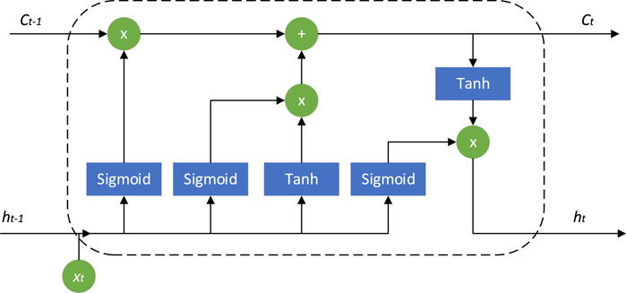
Figure 1. Memory cell structure diagram.

Translation: The Long Short-Term Memory (LSTM) network efficiently explores the temporal dependencies in the information of a time series by adding forget gates, input gates, and output gates in the hidden layer. At each time step, the LSTM unit receives the current data input x_j, the previous hidden state h_i-1, and the memory cell state C_t-1 through these gates. The computation process of LSTM is as follows:

In constructing an LSTM neural network, the forget gate helps LSTM determine which information will be removed from the memory cell state, and its formula as shown in Eq. 15:

$f_t=\sigma \left(W_{fx}{x}_t+W_{fh}{h}_{t-1}+b_f\right)(15)$

The input gate (i_t) is used to determine which new information will be stored in the new cell state (C_t). computation process as shown in formula 16:

$\begin{array}{l}{i}_t=\sigma \left(W_{ix}{x}_t+W_{ih}{h}_{t-1}+b_i\right)\\ g_t=\varphi \left(W_{gx}{x}_t+W_{gh}{h}_{t-1}+b_g\right)\\ C_t=C_{t-1}{f}_t+g_t{i}_t\end{array}(16)$

Translation: In the equation, g_t represents the candidate values to be added to the new cell state (C_t). C_t-1f_t determines how much information will be forgotten from C_t-1. The element-wise multiplication of g_ti_t is used to determine how much information will be added to the new cell state C_t.

The computation process for calculating h_t using the output gate (o_t) is as follows:

The CDNA module is added to the generating network optimization module. A set of convolutional kernels predicted by CDNA module is applied to the previous frame image to obtain multiple intermediate images with the same resolution, and their formula is and their formula can be expressed as 17:

$\begin{array}{l}{o}_t=\sigma \left(W_{ox}{x}_t+W_{oh}{h}_{t-1}+b_o\right)\\ h_t=o_t\varphi \left(C_t\right)\end{array}(17)$

In the equation, σ and ϕ represent the sigmoid and tanh activation functions, respectively. W_fx, W_fh, W_ix, W_ih, W_gx, W_gh, W_ox, and W_oh are weight matrices used for element-wise multiplication with the input x_t and the previous hidden state h_t-1 for the forget gate, input gate, input node, and output gate, respectively. b_f, b_t, b_g, and b₀ are the corresponding biases. f_t, i_t, g_t, o_t, C_t, and h_t represent the output results of the forget gate, input gate, input node, output gate, memory cell state, and hidden state, respectively.

3.3 CNN-LSTM network

CNNs (Convolutional Neural Networks) are primarily utilized for processing spatial features within input data. For charging load data, CNNs can capture spatial patterns across time and power dimensions. Through convolutional and pooling layers, CNNs automatically learn spatiotemporal characteristics of charging load data, such as distribution, fluctuation, and patterns of change. These features are crucial for predicting variations in charging loads. Convolution and pooling operations reduce the dimensionality of input data, extracting the most significant features. This process decreases the computational complexity of subsequent models while retaining essential spatial information.

LSTMs (Long Short-Term Memory networks), on the other hand, are designed to handle temporal sequence dependencies within input data. For charging load data, LSTMs can identify sequential patterns and long-term dependencies across the time dimension. With their internal gating mechanism, LSTMs effectively model and capture long-term dependencies in time series data. Specifically, for charging load data, LSTMs learn historical patterns and trends, enabling better predictions of future load variations. They also handle variable-length sequences, accommodating charging load data of different durations, thus offering flexibility for practical application scenarios.

The CNN-LSTM model combines the advantages of Convolutional Neural Networks (CNN) (Cheng et al., 2018) and Long Short-Term Memory Networks (LSTM) (Cheng, 2022). The prediction model is shown in Figure 2. By combining spectral clustering and the CNN-LSTM model, we can better differentiate different charging load patterns and train dedicated models for each pattern. This enables us to more accurately predict the electric vehicle charging demand under different charging load patterns, thereby improving the planning and management of charging infrastructure.

Figure 2

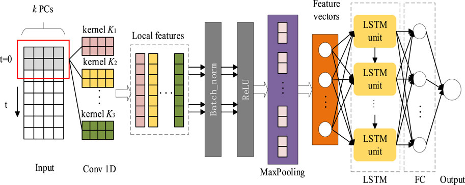
Figure 2. Convolutional long-term and short-term neural network prediction model.

The paper first uses a one-dimensional Convolutional Neural Network (CNN) to extract the hidden features of the time series vectors, which is set at the top layer of the entire prediction model. As shown in Figure 2, the CNN-LSTM prediction model consists of two main parts: a CNN neural network that extracts feature information from the original time series to obtain a sequence of feature information, and an LSTM network that predicts based on the obtained feature information sequence. Unlike traditional neural networks, the LSTM network has memory units in the hidden layer, where the information from the previous time step (t-1) is passed to the hidden layer neurons at time step t through the memory units, thus capturing long-term correlations between time series.

The training of the CNN-LSTM prediction model mainly involves two processes: forward propagation and backward propagation. In the forward propagation process, the main objective is to compute the error of the target loss function. The mathematical formula for the loss function is shown in Eq. 18. In the backward propagation process, the Adaptive Moment Estimation (ADAM) algorithm is used to optimize the network parameters.

$L=\frac{1}{F}{{\sum }_{T=1}^F\left({\mathrm{y}}_T-{\widehat{\mathrm{y}}}_T\right)}^2(18)$

In the equation, yT represents the true value of the charging load power at time step T, ${\widehat{\mathrm{y}}}_T$ represents the predicted value of the charging load power at time step T, and F represents the number of samples in the training sample set.

4 Electric vehicle charging load forecasting

Based on the aforementioned steps, this paper proposes a method for electric vehicle charging load forecasting using spectral clustering and deep learning networks.

First, the historical data of the target charging station is extracted using Monte Carlo simulation. The dataset needs to cover various dates, weather conditions, and other factors. The collected data is cleaned and normalized, and then Monte Carlo sampling is performed to generate a comprehensive and extensive dataset of electric vehicle charging load.

Next, the sampled dataset is subjected to spectral clustering. The clustering number K is iterated from 1 to n, and the optimal K value is selected based on the corresponding silhouette coefficient index and Davies-Bouldin index. The data is then divided into different clusters, and the cluster centroids of each category, representing samples with similar charging load characteristics, are obtained.

Finally, for each cluster, a CNN-LSTM model is constructed. The time series data is first subjected to convolution operations to extract spatiotemporal features from the charging load data. Through convolution and pooling operations, the CNN reduces the dimensions of the input data, extracts the most important features, and reduces the computational complexity of the model while retaining key spatial feature information. The LSTM captures the time series dependencies of the data and performs electric vehicle charging data forecasting using temporal regression. By combining spectral clustering and the CNN-LSTM model, different charging load patterns can be better differentiated, and dedicated models can be trained for each pattern. The structure of the electric vehicle charging load forecasting model based on spectral clustering and deep learning networks is shown in Figure 3.

Figure 3

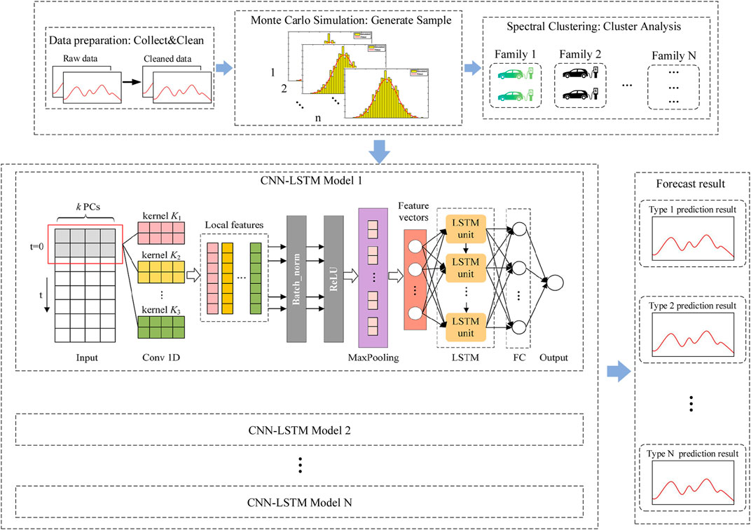
Figure 3. Framework diagram of electric vehicle charging load forecasting.

5 Case study

To validate the effectiveness of the proposed method, the experimental part selects a certain electric vehicle charging station in Pukou District, Nanjing, Jiangsu Province as the research object. The load data of this electric vehicle charging station has a sampling frequency of 5 min per data point, and the unit of the data is kW.

The prediction part of the experiment is the forecasting of electric vehicle charging load. The evaluation metrics used for the prediction results are Mean Absolute Error (MAE), Mean Squared Error (MSE), and Root Mean Squared Error (RMSE), as described in (Chai and Draxler, 2014). The calculation formulas for these metrics are shown in Eqs 19–21:

$e_{\text{MAE}}=\frac{1}{N}{\displaystyle \sum _{t=T+1}^{T+N}}\left|{\alpha }_t^s-{\widehat{\alpha }}_t^s\right|(19)$

$e_{\text{MSE}}=\frac{1}{N}{\displaystyle \sum _{t=T+1}^{T+N}}{\left({\alpha }_t^s-{\widehat{\alpha }}_t^s\right)}^2(20)$

$e_{\text{RMSE}}=\sqrt{\frac{1}{N}{\displaystyle \sum _{t=T+1}^{T+N}}{\left({\alpha }_t^s-{\widehat{\alpha }}_t^s\right)}^2}(21)$

In load forecasting, ${\alpha }_t^s$ = $p_t^s$ represents the true value of the load, and ${\widehat{\alpha }}_t^s$ = ${\widehat{p}}_t^s$ represents the predicted value of the load.

5.1 Charging load feature extraction

To validate the effectiveness of the proposed electric vehicle (EV) charging load prediction method based on spectral clustering and deep learning networks, historical charging load data from an EV charging station in Pukou District, Nanjing, Jiangsu Province, China, was employed. The historical load data covers the period from 0:00 on 14 July 2022, to 0:00 on 25 June 2023, with a sampling frequency of 5 min per data point, and the data is measured in kilowatts (kW).

Prior to load prediction, charging load feature extraction was conducted. Firstly, the historical load data was cleaned and normalized.

Subsequently, in the experiment, the processed data was directly subjected to spectral clustering without conducting Monte Carlo sampling simulation. The clustering results are presented in Table 1. From Table 1, it can be observed that there is a significant disparity in the number of data points among the three clustering labels. Label 1 has the highest count, with 94 data points, which even approaches three times the count of label 2. The substantial difference in data volume among the three labels, coupled with the inadequate data samples and incomplete coverage, may result in inconsistent model performance when training models for each label. Furthermore, it may lead to underfitting or overfitting issues. A smaller training dataset may fail to capture the distribution and patterns of the data adequately, thus resulting in subpar model performance. Conversely, a larger training dataset may lead to overfitting, where the model excessively fits the training data and struggles to generalize well to unseen data. Additionally, a smaller training dataset may lead to underfitting, where the model fails to sufficiently learn the data’s features and patterns, thereby resulting in inferior performance.

Table 1

Table 1. Non-Monte Carlo spectral clustering results.

Therefore, to address the issue of insufficient and incomplete data samples, this study performed Monte Carlo sampling simulation on the processed data to generate a diverse and comprehensive set of charging load samples.

The obtained samples from the simulation are saved as the experimental dataset, which consists of the simulated charging load data from 0:00 on 14 July 2022, to 0:00 on 15 June 2023, with a sampling frequency of 5 min per data point. This dataset is then used for spectral clustering operations according to the procedures described in Chapter 1.2.

During the spectral clustering process, a resolution coefficient ρ = 0.5 is used. The initial weight coefficient α is set as 0.05, while β is set as 0.95. The adjustment step τ for α and β is set as 0.01. K₀ starts from 2, and K_max is set as 20. The trends of the SC index and DBI index with the changing value of the clustering number K are shown in Figure 4. From Figure 4, it can be observed that the SC index and DBI index reach their optimal values when K = 3. Thus, the clustering number is determined as 3, and the cluster centroids are shown in Figure 5.

Figure 4

Figure 4. Change of SC and DBI indices with the amount of the amount K of the clusters.

Figure 5

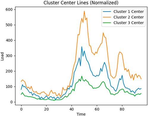
Figure 5. Cluster center line.

From Figure 5, it can be observed that the cluster centroids represent daily load curves with three distinct features, and there are significant differences between them. This can be mainly attributed to seasonal factors. In the summer, as shown in cluster 2, the load curve exhibits high volatility due to the hot weather, intensive operation of air conditioning systems in electric vehicles, increased power consumption, and higher charging frequency at the charging station. The load is particularly concentrated during the periods of midday to afternoon and evening rush hour.

On the other hand, clusters 1 and 3 exhibit similar daily charging load trends. Cluster 3 represents the spring and autumn seasons, where the charging load shows smoother and weaker fluctuations throughout the day, and the overall power consumption is lower compared to clusters 1 and 2. Cluster 1 represents the winter season, where the load curve is influenced by frequent operation of heating systems in electric vehicles due to the low temperature. However, the power consumption is significantly lower than that in the summer when air conditioning systems are heavily used, but higher than the charging load in the spring and autumn periods.

5.2 Electric vehicle charging load forecasting

Based on the results of spectral clustering, the method described in Section 3 is used to predict the output of distributed photovoltaics. In the power prediction part, the main purpose is to validate the effectiveness of the proposed method for electric vehicle charging load forecasting based on spectral clustering and deep learning networks. Therefore, this part of the experiment only compares the load data after spectral clustering with the proposed prediction method in this paper.

During the experiment, the clustered data is organized by class, and the data of each class is concatenated in chronological order to form a single time series data for each class, which serves as the experimental data for each class. The training set consists of 80% of the experimental data, and the remaining 20% is used as the test set.

The experiment was conducted using PyCharm on the Windows operating system. After establishing the CNN-LSTM network structure, the training effect of the model is evaluated by observing the loss values during training. The parameters are considered to be optimal for each class when the training loss value converges and becomes stable.

In the comparative experiment, we introduced the unreprocessed Monte Carlo spectral clustering-CNN-LSTM prediction model, the unclustered CNN-LSTM prediction model, the spectral clustering-RNN prediction model, and the spectral clustering-CNN-LSTM prediction model proposed in this paper for ablation experiments and comparative experiments. At the same time, we also introduced the unreprocessed Monte Carlo spectral clustering-CNN-LSTM prediction model to comprehensively study the differences in data sample size, clustering and unclustering, and CNN-LSTM and other neural network predictions.

Due to the different characteristics of each class, the prediction performance also varies, as shown in Figures 6–8 which depict the respective loss graphs during training.

Figure 6

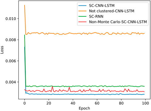
Figure 6. Loss plot for cluster label 0.

Figure 7

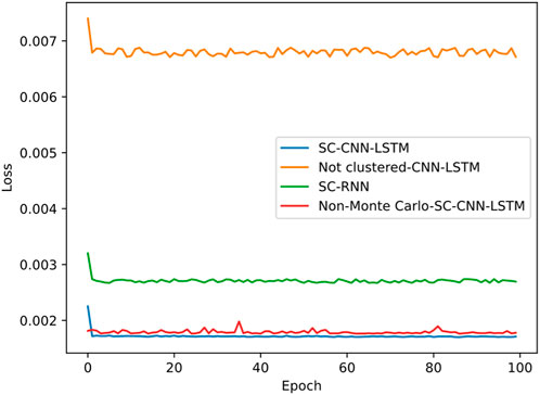
Figure 7. Loss plot for cluster label 1.

Figure 8

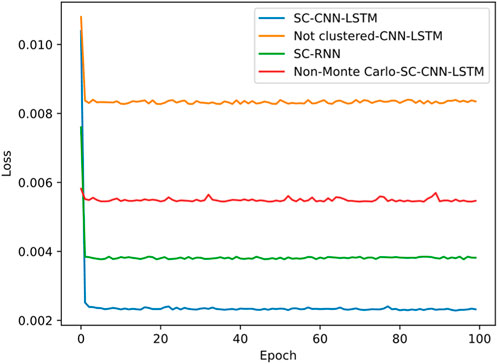
Figure 8. Loss plot for cluster label 2.

Figure 6 shows the loss curve for clustering label 0, Figure 7 for clustering label 1, and Figure 8 for clustering label 2. Each figure contains the loss curves for three methods. From Figures 6–8, it can be observed that the proposed spectral clustering-CNN-LSTM prediction model has significantly lower losses in each class compared to the other two contrastive methods. Additionally, the waveform tends to stabilize and converge more effectively in the proposed model. The loss of the spectral clustering-RNN prediction model, as shown in the figures, is higher than that of the proposed spectral clustering-CNN-LSTM prediction model, indicating the superior performance of CNN-LSTM. Moreover, the unclustered loss is notably higher than the other two methods, demonstrating that the algorithm’s loss is smaller and more likely to converge stably after clustering, highlighting the importance and necessity of the clustering algorithm. Since each cluster possesses distinct characteristics, the losses of the same methods vary between different label classes, leading to varying prediction performance.

Additionally, we also noted that in Figure 7, for label 1, the loss curve obtained from the unreprocessed Monte Carlo sampling simulation is similar to the loss curve described in this paper. The reason is that the data obtained from the non-sampled simulation itself has a relatively large amount of clustering label 1 data, and the model’s fitting ability is obviously better than the non-sampled simulation method for label 0 and label 1 models. However, for label 2, it can be seen from Section 5.1 that there are only 32 unlabeled data points for label 2 in the non-sampled Monte Carlo, which is significantly lower than the average level. This leads to the worst fitting ability of the model, and its loss value is significantly higher than the loss values of other methods in Figure 8. Therefore, it can be seen that Monte Carlo can solve the problem of insufficient data samples and incomplete coverage, which is of great significance for this experiment.

Subsequently, each class is compared separately using the predicted values from the four methods against the ground truth, and the results are presented in Figures 9–11.

Figure 9

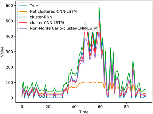
Figure 9. Predicted and true values at cluster label 0.

Figure 10

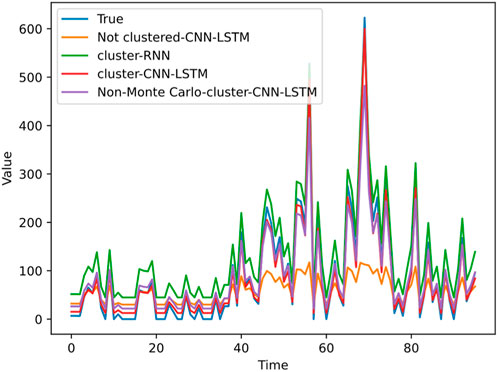
Figure 10. Predicted and true values at cluster label 1.

Figure 11

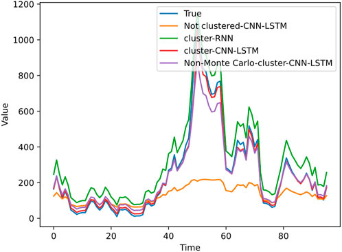
Figure 11. Predicted and true values at cluster label 2.

Figure 9 shows the predicted values and true values curves for the four methods when clustering label 0 is applied, Figure 10 shows the predicted values and true values curves for the four methods when clustering label 1 is applied, and Figure 11 shows the predicted values and true values curves for the four methods when clustering label 2 is applied. From the figures, it can be seen that the proposed electric vehicle charging load prediction model in this paper closely approximates the true photovoltaic output results, indicating the best prediction performance. The spectral clustering-RNN prediction model follows, followed by the unreprocessed Monte Carlo sampling simulation-SC-CNN-LSTM method, and the unclustered CNN-LSTM model has the poorest prediction performance. Comparing Figures 10, 11, it can be observed that Monte Carlo simulation makes the data more abundant and comprehensive, thereby improving the model’s fitting and generalization abilities. Meanwhile, spectral clustering plays a significant role in improving the prediction performance, and CNN-LSTM exhibits relatively good performance compared to other mainstream neural network algorithms.

The average absolute error, mean squared error, and root mean squared error for each class are presented in Tables 2–4, respectively.

Table 2

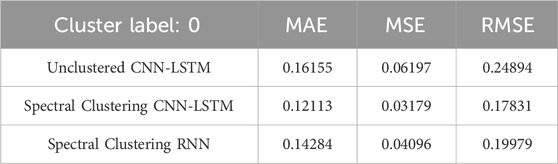
Table 2. Cluster label 0 evaluation index.

Table 3

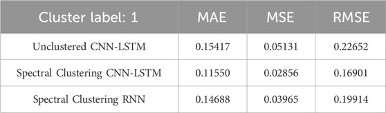
Table 3. Cluster label 1 evaluation index.

Table 4

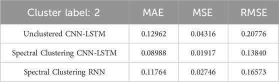
Table 4. Cluster label 2 evaluation index.

Table 2 shows the Mean Absolute Error (MAE), Mean Squared Error (MSE), and Root Mean Squared Error (RMSE) for the three algorithms when clustering label 0 is applied. From Table 1, it can be observed that the proposed Spectral Clustering CNN-LSTM method has the smallest errors. Specifically, both MAE and MSE are approximately 47% lower compared to the Unclustered CNN-LSTM algorithm and about 23% lower compared to the Spectral Clustering RNN method. The MAE value for the Spectral Clustering CNN-LSTM method is also the smallest among the three, indicating that for label 0, the proposed load prediction method exhibits the best evaluation metrics and prediction performance, thus highlighting the effectiveness of this approach.

Table 3 presents the evaluation metrics for the three algorithms when clustering label 1 is applied. From Table 3, it can be observed that the proposed Spectral Clustering CNN-LSTM method achieves approximately a 44% reduction in both Mean Absolute Error (MAE) and Mean Squared Error (MSE) compared to the Unclustered CNN-LSTM algorithm, and about a 28% reduction compared to the Spectral Clustering RNN method. The MAE value for the Spectral Clustering CNN-LSTM method is also the smallest among the three, at 11.55%. This indicates that for label 1, the proposed load prediction method exhibits the best evaluation metrics and prediction performance, further demonstrating the effectiveness of this approach.

Table 4 displays the evaluation metrics for the three algorithms when clustering label 2 is applied. The conclusion is consistent with Tables 2, 3. It is evident that for different labels, the proposed Spectral Clustering CNN-LSTM model consistently exhibits the best performance. Both spectral clustering and CNN-LSTM demonstrate significant importance in electric vehicle charging load prediction. This reinforces the effectiveness and significance of the proposed approach across various label classes.

In order to demonstrate the importance of Monte Carlo simulation on the data volume in this research, the experiments also involved the output of the original data without Monte Carlo sampling simulation. According to the clustering results in Table 1 in Section 5.1, CNN-LSTM prediction was performed, and the evaluation metrics are shown in Table 5. From Table 5, it can be observed that without Monte Carlo sampling, the model’s fitting ability was poor due to the small data volume of cluster label 2, resulting in underfitting and hence, lower evaluation metrics. Next is cluster label 0. Cluster label 1 had a more sufficient data volume, but its coverage was not comprehensive enough, resulting in slightly lower evaluation metrics compared to the Monte Carlo sampling simulated data. Overall, the prediction results without Monte Carlo sampling indicated that directly clustering and predicting the original data without Monte Carlo would result in poor model fitting performance. This also validates the capability of Monte Carlo simulation in addressing issues related to insufficient data samples and incomplete coverage, thereby improving the model’s fitting and generalization abilities. It is an indispensable part of this research.

Table 5

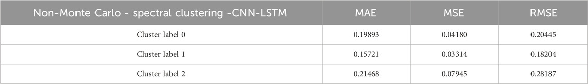
Table 5. Prediction results without Monte Carlo sampling simulation.

To validate the superior of the method proposed in this research, state-of-the-art EV charging load forecasting approaches are compared. And the comparing result are shown in Table 6. The baselines are eXtreme Gradient Boosting (XGBoost), Sequence to Sequence (seq2seq), Gated Recurrent Unit (GRU), Long Short-Term Memory (LSTM), Bidirectional Long Short-Term Memory (Bi-LSTM) respectively. The comparative experiments were performed on a mixed dataset, comprising both realistic and simulated data. The results are presented in Table 6.

Table 6

Table 6. Comparative analysis of baseline model performances on the mixed dataset.

Analysis of the data presented in Table 6 reveals that the method proposed in this study demonstrates superior performance compared to the baseline methods. This enhanced performance can be attributed to the integration of a hybrid deep learning approach, combining Convolutional Neural Networks (CNN) and Long Short-Term Memory (LSTM) networks. This combination effectively captures the characteristics of the training data and exhibits robust capabilities in handling time-series analysis.

6 Conclusion

The proposed electric vehicle (EV) charging load prediction method in this paper addresses the challenges related to the poor reliability, complexity, variability, and uncertainty of EV charging load data. The method combines spectral clustering with deep learning networks to achieve accurate and reliable EV charging load predictions.

In the feature extraction phase of EV charging load, historical data of EV loads in the target area are collected and cleaned. Monte Carlo sampling simulation is then performed to generate a set of simulated EV charging load data. By considering the distribution and statistical characteristics of the existing data, multiple simulated samples are generated using random sampling. The generated data is then subjected to spectral clustering analysis. Spectral clustering divides the simulated data into different clusters, where each cluster represents samples with similar charging load patterns.

In the EV charging load prediction phase, for each cluster, a corresponding CNN-LSTM model is constructed. The model is trained using the clustered and simulated charging load data as inputs, where the input is a time series of the sampled EV charging load data after clustering, and the output is the predicted charging load demand.

Finally, in the experimental part, various evaluation metrics are computed, and the prediction results from different models are compared against the real data. The proposed method’s computational accuracy and effectiveness in predicting EV charging load data are verified. The results demonstrate that the model provides reliable and accurate EV charging load predictions, offering valuable data support for the operation and management of EV charging stations.

Overall, the integration of spectral clustering and CNN-LSTM in this method contributes to handling the challenges posed by EV charging load data, enabling improved predictions and supporting more efficient management of EV charging infrastructure. In future work, the method proposed in this research should be validated across a broad range of geographical regions, utilizing sufficiently comprehensive datasets (Ma et al., 2020; Liu and Qin, 2023).

Data availability statement

The original contributions presented in the study are included in the article/Supplementary material, further inquiries can be directed to the corresponding author.

Author contributions

FX: Data curation, Writing–original draft. XY: Data curation, Writing–original draft. WB: Formal Analysis, Writing–review and editing. XR: Data curation, Writing–original draft. MF: Validation, Writing–review and editing. ZJ: Validation, Writing–review and editing.

Funding

The author(s) declare financial support was received for the research, authorship, and/or publication of this article. The authors declare that this study received funding from Science and Technology Project of State Grid Jiangsu Electric Power Co., Ltd. (J2022026). The funder was not involved in the study design, collection, analysis, interpretation of data, the writing of this article, or the decision to submit it for publication.

Conflict of interest

The authors declare that the research was conducted in the absence of any commercial or financial relationships that could be construed as a potential conflict of interest.

Publisher’s note

All claims expressed in this article are solely those of the authors and do not necessarily represent those of their affiliated organizations, or those of the publisher, the editors and the reviewers. Any product that may be evaluated in this article, or claim that may be made by its manufacturer, is not guaranteed or endorsed by the publisher.

References

Bai, Y., Zhou, Y., and Liu, J. (2022). Clustering analysis of daily load curve based on deep convolution embedding. Power Syst. Technol. 46 (6), 2104–2113. doi:10.13335/j.1000-3673.pst.2021.1080

CrossRef Full Text | Google Scholar

Chai, T., and Draxler, R. R. (2014). Root mean square error (RMSE) or mean absolute error (MAE)? Arguments against avoiding RMSE in the literature. Geosci. Model Dev. 7 (3), 1247–1250. doi:10.5194/gmd-7-1247-2014

CrossRef Full Text | Google Scholar

Chen, Z., Zhu, J., Wang, Y., and Lin, C., (2022). Electric vehicle charging load modeling based on consistency K-means clustering. Mod. Electr. Power 39 (3), 338–348. doi:10.19725/j.cnki.1007-2322.2021.0107

CrossRef Full Text | Google Scholar

Cheng, D. (2022). Review on LSTM research status. Inf. Syst. Eng. 52 (1), 149–152.

Google Scholar

Cheng, J., Wang, P., Li, G., Hu, Q. h., and Lu, H. q. (2018). Recent advances in efficient computation of deep convolutional neural networks. Front. Inf. Technol. Electron. Eng. 19 (1), 64–77. doi:10.1631/fitee.1700789

CrossRef Full Text | Google Scholar

Deng, Y., Huang, Y., and Huang, Z. (2021). Electric vehicle charging and discharging capacity prediction based on random forest algorithm. Power Syst. Autom. 45 (21), 181–188.

Google Scholar

Guanyuan, W., Wang, G., and Ruan, G., 2023, Review of intelligent decision and optimization for electric vehicle charging station site selection. Comput. Eng. Appl. 14.

Google Scholar

Huang, D., Zhuang, X., Hu, A., Sun, J., Shi, S., Sun, Y., et al. (2021). Short-term load forecasting based on grey relational analysis and K-means clustering. Electr. Power Constr. 42 (7), 110–117.

Google Scholar

Liu, Q., and Qi, Z. (2014). Electric vehicle load prediction modeling based on Monte Carlo method. Power Sci. Eng. 30 (10), 14–19.

Google Scholar

Liu, S., and Qin, Z. (2023). Joint optimization method for load frequency control with electric vehicle clusters. Electr. Switchg. 61 (1), 7–16.

Google Scholar

Liu, W., Xu, X., and Zhou, Xi (2014). Daily load forecasting for pure electric bus charging/swapping stations based on support vector machine. Electr. Power Autom. Equip. 34 (11), 41–47.

Google Scholar

Lu, J., Zhang, Q., Yang, Z., Tu, M., Lu, J., Peng, H., et al. (2019). Short-term load forecasting method based on hybrid CNN-LSTM neural network model. Automation Electr. Power Syst. 43 (8), 131–137.

Google Scholar

Luo, H., Ruan, J., and Li, F. (2014). A fuzzy evaluation and AHP based method for the energy efficiency evaluation of EV charging station. J. Comput. 9 (5). doi:10.4304/jcp.9.5.1185-1192

CrossRef Full Text | Google Scholar

Ma, Y., Yang, Z., and Li, H. (2020). Innovation product diffusion prediction based on Bass model and LTV. J. Liaocheng Univ. Nat. Sci. Ed. 33 (04), 26–32. doi:10.19728/j.issn1672-6634.2020.04.004

CrossRef Full Text | Google Scholar

Mohammed, N. S., and Mohammed, H. E. (2022). Accurate photovoltaic power prediction models based on deep convolutional neural networks and gated recurrent units. Energy Sources, Part A Recovery, Util. Environ. Eff. 44 (3), 6303–6320. doi:10.1080/15567036.2022.2097751

CrossRef Full Text | Google Scholar

Peng, S., Huang, S., Li, B., Zheng, G., and Zhang, H. (2020). Charging pile load forecasting based on deep learning quantile regression model. Power Syst. Prot. Control 48 (2), 44–50. doi:10.19783/j.cnki.pspc.190289

CrossRef Full Text | Google Scholar

Ren, M., Jiang, M., Song, Y., Peng, J., Chen, S., Li, S., et al. (2023). City electric vehicle charging load forecasting based on Monte Carlo method. Electr. Eng. 42 (4), 18–23.

Google Scholar

Shi, L., Li, Y., Liu, J., Wang, Z., and Wang, W. (2023). Improved GRU method for ultra-short-term charging load forecasting of electric vehicle charging stations. Power Supply Demand 40 (6), 42–47. doi:10.19421/j.cnki.1006-6357.2023.06.006

CrossRef Full Text | Google Scholar

Wang, S., Liu, J., Zheng, F., and Pan, W. (2023). A survey on machine learning based spectral clustering. J. Comput. Sci. 50 (1), 9–17.

Google Scholar

Yang, Y., and Wang, Y. (2014). Simulated annealing spectral clustering algorithm for image segmentation. Syst. Eng. Electron. Engl. Ed. 25, 514–522. doi:10.1109/jsee.2014.00059

CrossRef Full Text | Google Scholar

Zhou, C., Chen, Y., and Zhu, Y. (2023). Particle K-means clustering algorithm. J. Comput. Eng. Appl. 59 (13), 317–324.

Google Scholar