Power quality improvement using a 31-level multi-level inverter with bio-inspired optimization approach

In recent years, the power quality (PQ) improvements have been explored through various approaches. The employment of electronic devices with renewable energy sources has expanded the harmonics level of voltage and current. Due to harmonics, the PQ of a specific electrical system gets affected. At critical load conditions, the traditional PQ mitigation approaches fail to develop the performance of the system. Therefore, in this work, the Spider Monkey Optimization convolutional neural network (SM-CNN)-based 31-level multilevel inverter (MLI) is used. This method balances the reactive power demands and enhances real power in the grid-tied photovoltaic (PV) system. The maximum power point tracking (MPPT) algorithm depending on radial basis function neural networks (RBFNNs) is used to maximize PV power. For strengthening the voltage level of the PV and to generate higher DC voltage with a minimized switching loss, an integrated boost fly back converter (IBFC) is introduced. The presented technique is implemented in the MATLAB/Simulink platform to figure out the estimation of PQ issues. The suggested MLI lessens the total harmonic distortion (THD) value to 2.45% with an improved power factor.

1 Introduction

In developing technologies, the issue of power electronic devices has shown a greater surge because of the exploitation in real-time applications. Generally, several types of controllers are used to mitigate different power quality (PQ) issues (Babu et al., 2020a). The rapid consolidation of photovoltaics (PV) is mostly based on improvements in PQ and global radiation technology (Ray et al., 2018). Power is converted from DC to AC by use of an inverter and a distribution system. The majority of voltage and current distortion has an impact on the system’s performance when it is linked to the grid. As a result of highly volatile devices coupled with an increase in the demand for nonlinear loads, the effectiveness of the system and the power network with regard to PQ is also affected (Badoni et al., 2021).

The unique functions of the PQ impact are consumers and utility equipment. By including renewable energy sources (RES) in the grid, the PQ of the system might be increased. Based on the coupled RES and nonlinear loads, the negative impacts on the system’s PQ are improved in this case. A renewable energy source contributes to the amount of reactive power on the line, and the associated harmonics are determined by nonlinear loads on the grid (Babu et al., 2020b; Golla et al., 2021; Ray et al., 2021). Many other RES-based technologies have been created during the last few years. Some of those sources are becoming more affordable very quickly, and others are widely recognized as low-cost options for grid-related applications (Rajesh et al., 2021).

The output voltage of boost-type converters can be boosted above the input voltage. Nevertheless, because of the internal losses, output voltage, and current stresses suffered by semiconductors, they present a gain restriction (Spiazzi et al., 2010). A high-frequency transformer connected to a flyback converter can be used as a way to receive significantly more voltage. However, because of the energy stored by the converter in its leakage inductance, when blocking voltage is present, the power main switch frequently shows a high reverse voltage (Chen et al., 2015; Shitole et al., 2017).

As a result, using integrated converters is necessary for the purpose of increasing costs and lowering efficiency. Moreover, during commutations, high conversion exposes the diode output to maximum voltage peaks. Furthermore, conventional converters have a limited duty ratio but can increase the output voltage. Furthermore, output voltage and switching stress are also both close. As a result, the given output voltage is considered the duty cycle with a lower value, increasing the converter’s efficiency (Hu et al., 2014; Pathy et al., 2016; Shen and Chiu, 2016; Banaei et al., 2019). Therefore, in order to overcome the above issues, the integrated boost-flyback converter (IBFC) is used in this study. The proposed IBFC effectively stabilizes the PV output voltage.

The maximum power extraction method is a main consideration in PV system electricity generation for improving the effectiveness of non-uniform solar irradiance and shading. Overall, numerous control techniques for a grid-coordinated PV system have been proposed (Bouselham et al., 2017). The most commonly used MPPT algorithms in both huge and small-sized PV applications are fuzzy logic control, perturb and observe (P&O), and incremental conductance. It is a difficult task to maintain synchronization, reliability, and overall system behavior in the grid connection (Chandra and Gaur, 2020; Prasad et al., 2021). As a consequence, an efficient control mechanism is required to control PQ issues in a PV system. Thus, the effective RBFNN-MPPT is employed to separate more power from the PV system.

Domestic and industrial appliances have seen enormous growth over the past few years. Power systems with defects that cause damage produce their elements as an outcome of the overheating process (Kumar et al., 2018; Dhanamjayulu et al., 2019; Khare et al., 2020; Lal and Thankachan, 2021). Additionally, there are certain common problems in these power systems, such as harmonic distortion, voltage sag, transient, and spikes (Arjunagi and Patil, 2021; Parida et al., 2021; Ramasamy and Perumal, 2021; Aarthi et al., 2023). With the help of Spider Monkey optimization CNN, MLI tackles the aforementioned issues and provides a high output voltage. The power quality should be considered to improve the performance based on renewable energy using DC–DC converters, and bridge controllers are used to optimize the energy (Kumar et al., 2012; Shimi et al., 2013).

By the main considerations of various problems, the power quality disturbances are classified by using neural network classifiers, but they mostly conflict massive distortions that occur and fail to improve the performance of power quality (Saravanakumar and Saravana kumar, 2023). However, in some cases, the new learning algorithms are used based on the deep learning system by concerning power quality systems [29]. The CNN model makes deforming scaling learning techniques to classify the distortion, but learning weights are mitigated to adjust the bias weight of power quality elements to improve the performance.

In this paper, the efficient RBFNN-based MPPT is deployed for improving the performance of the grid-tied PV system from PQ issues. The IBFC is used to boost the level of voltage in the PV system. By using the SM-CNN control approach for 31-level MLI, the PQ is successfully improved, and this inverter takes parallel processing PQ difficulties to easily manage the power consumption. Hence, the suggested approach is used to provide the system with enhanced PQ and a reduced THD of 2.45%.

2 Proposed system

The block diagram of the suggested methodology is demonstrated in Figure 1. The grid coordinated with the solar system consists of the PV array, IBFC, 31-level MLI, and LC filter.

Figure 1

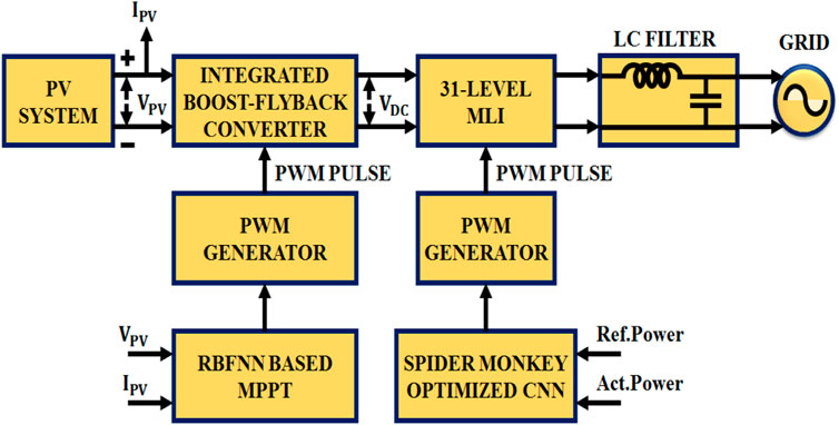
Figure 1. Block diagram of suggested Methodology.

For applying the RBFNN-based MPPT algorithm, the highest power is extracted from the PV system, and it is also utilized to strengthen the power conversion efficiency in the solar panel. A single PV panel produces a limited amount of electricity, necessitating the use of a large number of PV panels. The boost-flyback converter is integrated to circumvent this problem, which in turn produces a stable output. The MLI converts the power, in the form of DC into AC, and it is transformed into the grid (i.e., load). The enhanced output from the converter is fed into a 31-level MLI that enhances the PQ and minimizes the lower-order harmonics, with the assistance of SM-CNN.

3 Proposed system modeling

3.1 Modeling of the PV system

The majority of PV arrays include an inverter to transform DC into alternating current, which may be used to power loads like motors, lights, and other appliances. The individual components of a PV array are normally connected in parallel after the modules are typically connected in series to achieve the necessary voltages. The corresponding circuit diagram for a PV cell is shown in Figure 2.

Figure 2

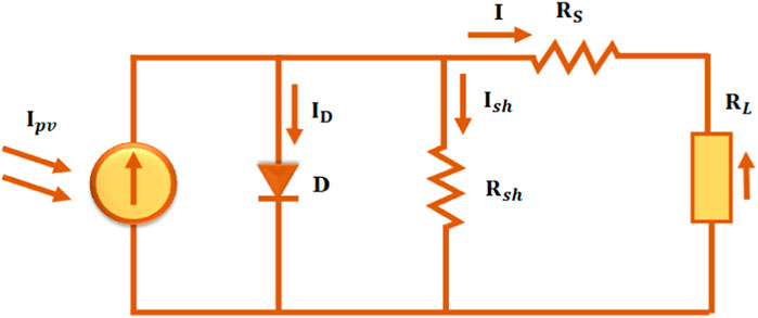
Figure 2. Circuit diagram for PV cell.

A current source in parallel with a diode models an ideal. Nevertheless, no solar cell is perfect, so shunt and series resistances are included in the model, as illustrated in the PV cell schematic above. $R_S$ is the intrinsic series resistance, which has a very small value. $R_{Sh}$ is the equivalent shunt resistance, and it is extremely high.

Applying Kirchhoff’s law to the node where $I_{pv}$, diode $R_{Sh}$, and $R_S$ reach yields the following equation:

$I_{pv}=I_D+I_{sh}+I.(1)$

The PV current equation is given as

$I=I_{pv}-I_{sh}-I_D,(2)$

where $I_{pv}$ is the insolation current, $I$ represents the cell current, $I_O$ is reverse saturation current, $V$ denotes the cell voltage, and $R_S$ indicates the series resistance. According to the cell current, the parallel resistance remains to balance the isolation current shown in Eq. 2.

$I=I_{pv}-I_O.\left[\exp \left(V+I.\frac{R_S}{V_T}\right)-1\right]-\left[V+I.\frac{R_S}{R_{Sh}}\right].(3)$

$R_{Sh}$ represents the parallel resistance, $V_T$ represents the thermal voltage $\left(KT/q\right)$, $K$ represents the Boltzmann constant, $T$ represents the temperature in Kelvin, and $q$ represents the charge of an electron. The forthcoming section provides the detailed description about the RBFNN-MPPT algorithm, which separates the maximum power from the PV panel.

3.2 Model of the radial basis function neural network-based MPPT technique

Figure 3 demonstrates the architecture for the RBFNN-based MPPT algorithm. The proposed RBFNN-MPPT is a three-layer network with a hidden layer, input layer, and output layer.

Figure 3

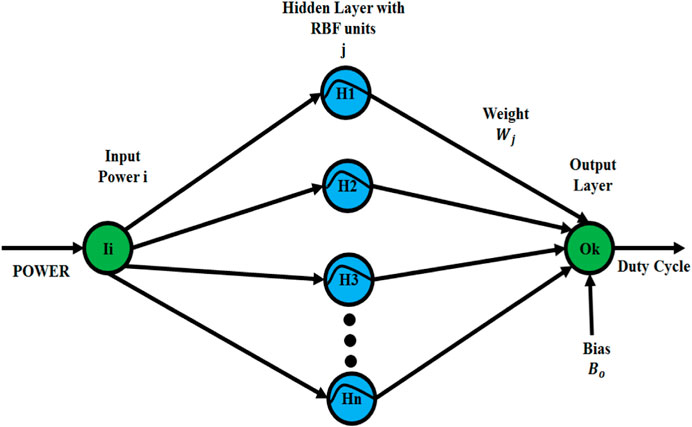
Figure 3. RBFNN-based MPPT algorithm.

It is an algorithm for supervised learning, which is employed to train multi-layer activation functions. When a specific set of inputs (power) is applied to the RBFNN-based MPPT technique, it produces the expected output (duty cycle) by fine-tuning its weights. Using PV module power and converter duty cycle as input variables and irradiance variations as the output variables, the RBFNN is trained. The parameters used in the RBFNN training are listed in Table 1.

Table 1

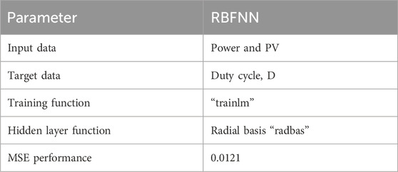
Table 1. Parameter specification.

Steps for the RBFNN

Step 1:. Generation of random weights to small random values to make sure t hat the network is unsaturated by large weight value.

Step 2:. A training pair from the training set is selected

Step 3:. The input vector to the network input is applied

Step 4:. The network output is calculated

Step 5:. Error is computed as the subtraction between the network output and desired output.

Step 6:. Network weights are adjusted in order to minimize the error.

Step 7:. Return to steps 2-6 for the individual input-output pair of the training set until the error for the whole system is tolerabley.

The RBFNN’s hidden layer has unique activation functions including Gaussian, multi-quadratics, and inverse multiquadratics. When compared to the traditional BPNN, the RBFNN is a better activation function with reduced distance from function establishments.

The hidden layer is composed of a Gaussian activation function that is focused in feature space on a vector. There are no extra weights from the input layer to the hidden layer. The input layer is delivered directly to the $j-th$ Gaussian hidden unit. The RBF’s $k-th$ unit output is indicated as follows:

$O_k=B_O+{\displaystyle {\sum }_{j=1}^h}{W}_{jk}*H_j,(4)$

where $H_j$ represents the radial basis output of the $j-th$ hidden unit and is given by $H_j=f\left(\left|\left|I-c_j\right|\right|\right)$ Here, $c\in R$ refers to the center of the RBF with radius $r$.

$f\left(x\right)=e^{\left(\frac{{\left|\left|I_i-c_j\right|\right|}^2}{r^2}\right)}.(5)$

3.2.1 Performance testing

The mean squared error (MSE) impacts the performance of the NN. By modifying the output-layer weight $W_{jk}$, the MSE is minimized depending on the inputs $I$ and $T$ target vector is presented as follows:

$E=1/m{\displaystyle {\sum }_{k=1}^m}{\left(T_k-O_k\right)}^2,(6)$

$\text{where\hspace{0.17em}}t\left(k\right)ando\left(k\right)$ represent a target and network output $kth$ sample, respectively, and $m$ represents the total training patterns.

Table 2 represents the parameter specification for RBFNN MPPT techniques. The highest power attained from the PV system is enhanced with the advisable IBFC, which is employed to convert the PV output voltage into an AC form with higher efficiency and low switching losses.

Table 2

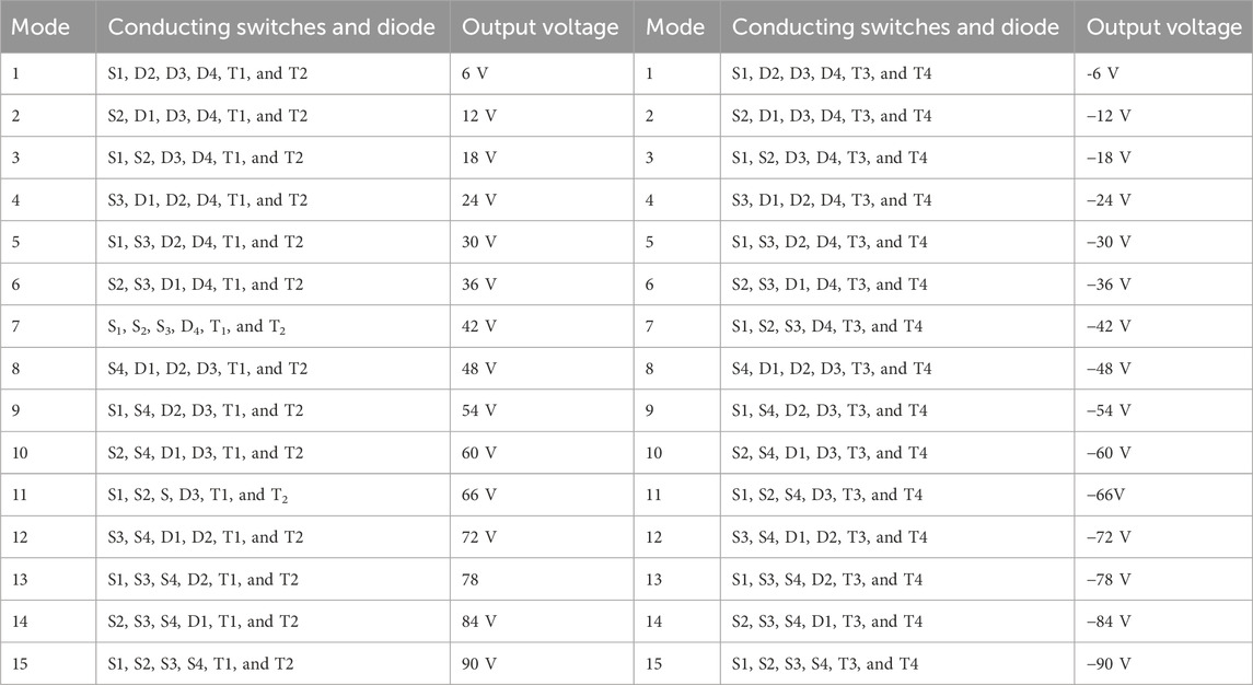
Table 2. Modes of operation.

3.2.1.1 Modeling OF IBFC

Figure 1 shows that the IBFC shares the power IGBT switch and the inductor to integrate a boost and flyback converter.

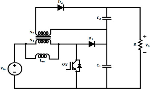
The inductor employed in this instance is a type of a linked inductor, which has two windings wound around a single magnetic core. $L_m$ represents the connected inductor’s magnetizing inductance. There are, respectively, $N_1$ and $N_2$ turns in the primary and secondary windings. $C_T$ and $C_2$ are connected in series to produce the IBFC output. The magnetizing current $i_{Lm}$ runs continuously and stays above 0 throughout a switching cycle in the continuous conduction mode (CCM). The operation of the IBFC can be divided into stages.

3.2.1.2 Stage 1

While $SW$ is activated, $D_1$ and $D_2$ are reverse-biased. $V_{in}$ is used to power the linked inductor’s primary winding, $i_{Lm}$ increases linearly, and $L_m$ stores the energy. The linked inductor’s primary and secondary currents, $i_1$ and $i_2$, respectively, are both 0 since D2 is reverse-biased. The load resistance, $R$, discharges $C_1$ and $C_2$ throughout this time, supplying the load current.

3.2.1.3 Stage 2

Figure 4 when $SW$ is disabled, $i_{Lm}$ continues to flow in the same direction by compelling $D_1$ and $D_2$ to conduct. During this time, the energy held in $L_m$ is released to charge $C_1$ and $C_2$ as $i_{Lm}$ linearly diminishes.

Figure 4

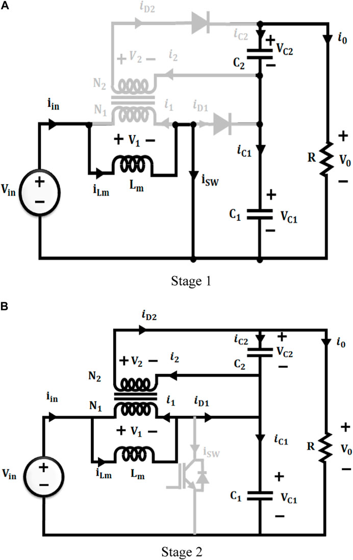
Figure 4. IBFC.

With the use of this approximation, the current waveform analysis and device ratings, such as $SW,D_1,and{D}_2$, are made easier.

The following equation represents the voltage gain of the IBFC as follows:

$\frac{V_O}{V_{in}}=\frac{1+nD}{1-D},(7)$

$V_O=V_{in}\left(\frac{1+nD}{1-D}\right),(8)$

where $D$ is the duty cycle of the $SW$ and $n=N_1/N_2$ is the linked inductor’s turn ratio. By modifying the duty ratio $D$ of the switch, the average output voltage of the IBFC is changed.

3.2.2 Modeling of the 31-level MLI

Asymmetric semiconductor devices using the same voltage sources and quantity can also produce high output levels when compared to their symmetric counterparts. The MLI structure, constructed with an H-bridge inverter circuit defined as the polarity generation circuit and an asymmetric fundamental circuit called as the level generator unit, is illustrated in Figure 5. Switches in the polarity generation circuit, especially contrasted to other switches in the level generation unit, are under more stress.

Figure 5

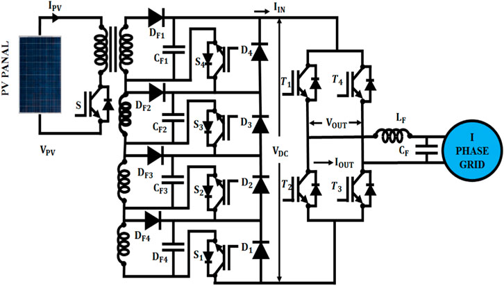
Figure 5. Proposed MLI.

The circuit contains an equal number of driver circuits and IGBTs as all of its semiconductor switching components are positioned in the same direction. The switching losses in a multilevel inverter circuit depend on three different parameters: switching frequency, current, and blocking voltage. The locations of each and every switch in the level generation unit are displayed in Table 3. A total of 15 levels are generated using the level generation units $S_1,S_2,S_3,and{S}_4$ and the polarity generation units $T_1$ and $T_2$. Switching OFF $S_1,S_2,S_3,and{S}_4$ results in the 0 level. Half cycles, both positive and negative, are also symmetrical.

Table 3

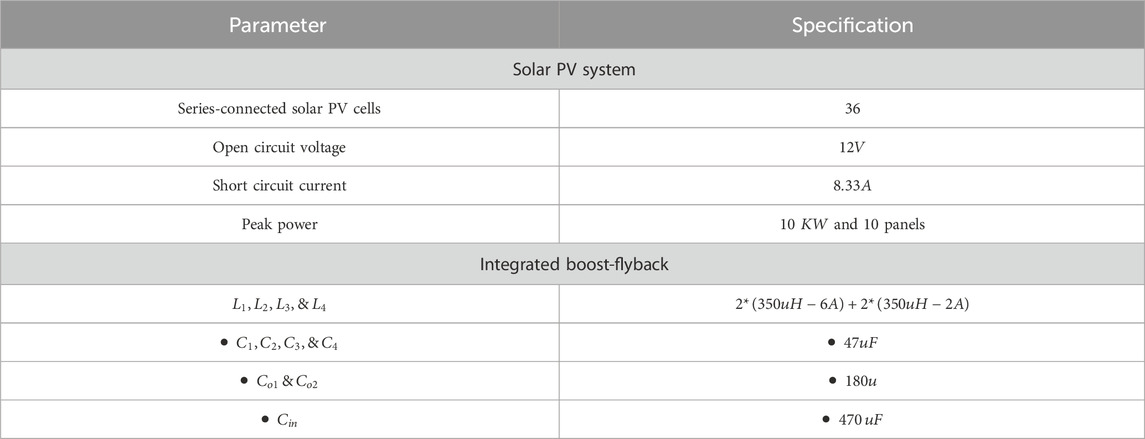
Table 3. Design parameter.

As an illustration, the switches $S_{1}and{S}_2$ are turned ON, and state 3 of the diodes $D_3$ and $D_4$ are forward-biased. In the positive half-cycle, $V_O=V_1+V_2$ is obtained. This method is repeated for each additional state to achieve the output voltage values.

In a positive cycle, the H-bridge inverter’s switches $T_1$ and $T_2$ are turned $ON$, while $T_3$ and $T_4$ are turned $OFF$. $T_1$ and $T_2$ are turned $OFF$, while $T_3$ and $T_4$ are turned $ON$ during the negative cycle. The following Table 3 demonstrates the 31-MLI’s method of operation.

The circuit is going to operate in mode 1, and the amplitude of 6 V will now be linked to the grid through the inverter switches $T_1$ and $T_2$ during the positive half-cycle when the switches $S_1$, $D_2$, $D_3$, and $D_4$ of the multiplier are switched $ON$. The circuit will transition to mode 2, and the output voltage of 12 V will be accessible at the inverter output when switches $S_2$, $D_1,$ $D_3$, and $D_4$ are turned $ON$. Similarly, by turning on the switches $S_1$, $S_2,D_3$, and $D_4$ of the multiplier cell in mode 3, the output of 18 V will be made available. The switches are activated in this order until all 15 modes have been used. For negative cycles, the same switching sequence is repeated.

3.2.3 SM optimized CNN

3.2.3.1 CNN

The CNN classifier efficiently differentiates the harmonics with the help of the features including standard deviation, mean, entropy, energy, and log-entropy. The feedforward network of the CNN basically has three layers, such as maximum, pooling, and convolutional layers, which are fully connected. The CNN architecture is illustrated in Figure 5.

The backpropagation method is used to train the parameters. The factor of two values is down-sampled by pooling layers, which is regarded as the down-sampling layer, and the maximum value of the convolutional layer is sent to the next layer. The number of training samples and times is reduced by this proposed strategy. These samples are carried on to the following layer, which is fully connected and has multiple hidden layers. Weights are used to connect the hidden and output layers, the final output classifier layer, and the pooled samples to a fully connected network. The forward and backpropagation are the two steps of the training process, where forward propagation provides the actual input data and backpropagation updates the training parameters.

Using all of the input coefficients has a negative influence on the classification accuracy every time. As a result, the chosen coefficients mean $\left(M\right)$, standard deviation $\left(SD\right.$), energy ($\left.E\right)$, entropy ($\left.ET\right)$, and log-energy entropy $\left(LE\right)$ are eliminated to reduce complexity and improve classification accuracy. The primary component expressions are described as follows:

Mean

$M_{ki}=-\frac{1}{N}{\displaystyle {\sum }_{j=1}^N}{X}_{ij}.(9)$

Energy

$K_{ki}={\displaystyle {\sum }_{j=1}^N}\left({\left|X_{ij}\right|}^2\right).(10)$

Standard deviation

${\sigma }_{ki}={\left(\frac{1}{N}{\displaystyle {\sum }_{j=1}^N}{\left(X_{ij}-{\mu }_i\right)}^2\right)}^{\frac{1}{2}}.(11)$

Entropy

${ET}_{ki}=-{\displaystyle {\sum }_{j=1}^N}{X_{ij}}^2\log \left({X_{ij}}^2\right).(12)$

Log-energy entropy

${LE}_{ki}=-{\displaystyle {\sum }_{j=1}^N}\log \left({X_{ij}}^2\right).(13)$

In this paper, the reference and real signals are transmitted to the CNN classifier to reduce the harmonics and provide reference power to the PWM generator that produces gating pulses for the 31-level MLI. Furthermore, the CNN has to be optimized to enhance the control performance of the MLI.

4 SMO algorithm

The SMO methodology is a metaheuristic method that uses fission and fusion swarm intelligence for foraging. This algorithm is inspired from the behavior of spider monkey. The following are six iterative collaborative phases, and the SMO method relies on trial and error.

4.1 Initializing

The SMO initializes each ${SM}_p$ using Eq. 14

${SM}_{pq}={SM}_{minq}+UR\left(0,1\right)\times \left({SM}_{maxq}-{SM}_{minq}\right),(14)$

where ${SM}_{pq}$ is the $qth$ dimension’s $pthSM,$ for random, the upper and lower bounds of ${SM}_p$ of ${SM}_{minq}$ and ${SM}_{maxq}$ in the $qth$ direction, respectively. The number of $UR$ is between [0, 1], with a uniform distribution.

4.2 Local leader phase)

$SM$ includes the historical occurrences of local group members and leaders to shift the place. If the new position value is higher than the past one, the $SM$ location of the $lth$ local group is updated.

${SM}_{newpq}={SM}_{pq}+UR\left(0,1\right)\times \left({LL}_{lq}-{SM}_{pq}\right)+UR\left(-1,1\right)\times \left({SM}_{rq}-{SM}_{pq}\right).(15)$

The local group $lth$ of the $qth$ dimension is selected for $lth$. $SM$ is random and is represented as ${SM}_{rq}$, such that $r,p$. ${LL}_{lq}$ is the $qth$ dimension of the $lth$ local group leader location.

4.3 Global leader phase

Following LLP, the GLP is initiated to update the location. Equation 16 provides the location update as follows:

${SM}_{newpq}={SM}_{pq}+UR\left(0,1\right)\times \left({GL}_{lq}-{SM}_{pq}\right)+UR\left(-1,1\right)\times \left({SM}_{rq}-{SM}_{pq}\right),(16)$

where ${GL}_{lq}$ represents the $qth$ dimension of the GLP and $q$ is a randomly chosen index between $1andM$.

4.4 Global leader learning phase

By utilizing the strategy of greedy selection, GLL is updated. The new SM depends on the country with the fittest people in the world. If updates are discovered, the global limit count (GLC) is increased and the value of the global leader is applied to the optimum setting.

4.5 Local leader learning phase

The $SM$ location is updated with the position of the local leader for optimal fitness in a specific group. The ideal location is given to the local leader. If no updates are found, an increment of 1 is applied to the limit count.

4.6 Local leader decision phase

When a local leader does not update its location or outdated from global and local leaders depending on $P_r$ using Eq. 17, the candidates of the local group change the position at a random step 1.

${SM}_{newpq}={SM}_{pq}+UR\left(0,1\right)\times \left({GL}_{lq}-{SM}_{pq}\right)+UR\left(0,1\right)\times \left({SM}_{rq}-{LL}_{pq}\right).(17)$

4.7 Global leader decision phase

In accordance with GLD, the population is split into smaller groups. For the global leader limit, the location value is unchanged. The dividing process starts after there are as many groups (MG) as possible. For the newly created group, a local leader is selected during each cycle. It does not modify its position until the allowable maximum is reached, at which point it tries to merge all of the permitted groups into a single group. The maximum number of permitted groups is established.

4.8 Gaussian mutation

In complex iterative optimization situations, the SMO approach is imprisoned in the local best value. The algorithm solution value does not vary throughout the iteration. This approach leaves the location of the local optimum, adds GM and random perturbation, and then extends to execute the algorithm in order to enhance the algorithm probability and algorithm deficiency. Equation 18 provides the formula for the Gaussian mutation.

$x^{i,iter+1}=\left\{\begin{array}{ll}{x}^{i,iter}+rand& ifr\ge 0.2\\ x^{i,iter}\times Gaussian\left(\mu ,\sigma \right)& otherwise\end{array}\right..(18)$

where rand represents a random number between [0, 1], and $r_j$ represents the probability of random perturbation or Gaussian mutation selection. Equation 19 provides the Gaussian variation distribution.

$Gaussian\left(\mu ,\sigma \right)=\left(\frac{1}{\sqrt{2\pi \sigma }}\right)\exp \left(-\frac{{\left(x-\mu \right)}^2}{2{\sigma }^2}\right),(19)$

where ${\sigma }^2$ stands for the variance and $\mu$ stands for the mean value. With the support of SMO, the CNN parameters are optimally tuned for the generation of improved THD and unity power factor.

5 Results and Discussion

This proposed work aimed at the improvement of an efficient spider monkey optimization CNN, which is deployed to improve the PQ in the grid-tied PV system. In addition, the RBFFN-based MPPT algorithm is employed to track the highest power from the PV system. The suggested control technique is verified using the MATLAB platform. Table 4 represents the parameter specification for the proposed system.

Table 4

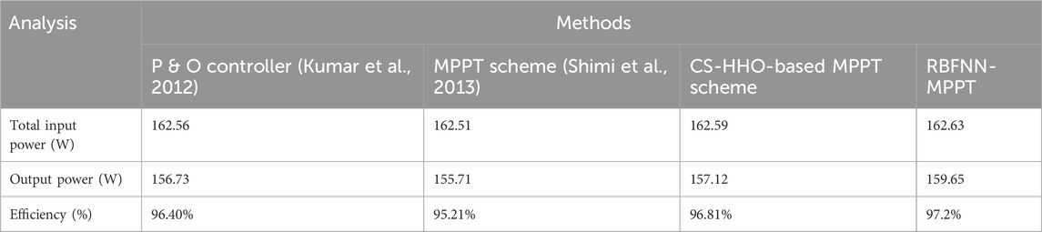
Table 4. Efficiency analysis.

A temperature variation of 0.1 s is introduced, as shown in Figure 6A, to calculate the efficiency of the suggested technique in handling the intermittent nature of the PV system. At this same moment, the temperature suddenly increases from 25°C to 35°C. Similar to how temperature varies, Figure 6B shows that solar irradiation varies from 800 W/sq.m to 1000 W/sq.m.

Figure 6

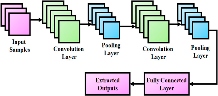
Figure 6. CNN Architecture.

Figure 7 displays the solar panel voltage and currents as a variation in temperature. Due to operating conditions, the voltage is suddenly increased from 58 V to 72 V; similarly, the current increases to 15 A, afterward, the current remains constant at 0.1 s.

Figure 7

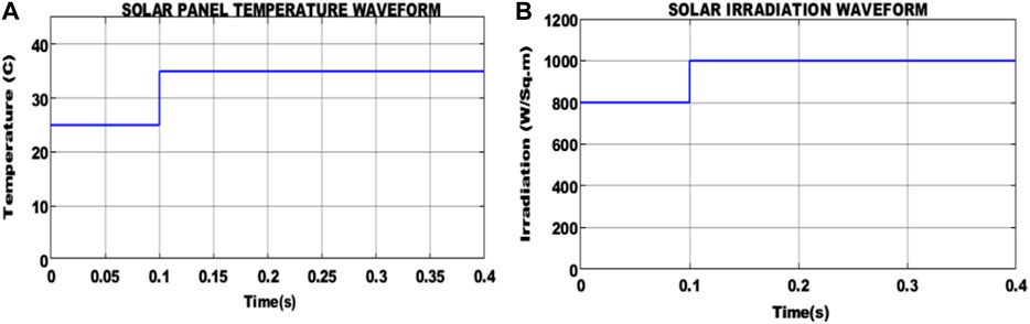
Figure 7. (A) Temperature and (B) irradiation waveforms for the solar panel.

The waveform that represents the voltage output of the IBFC is presented in Figure 8A. From that waveform, the voltage of 300 V is achieved at 0.2 s, and Figure 8B shows output current variations until 0.1 s, after which the stable value of 2.5 A is maintained.

Figure 8

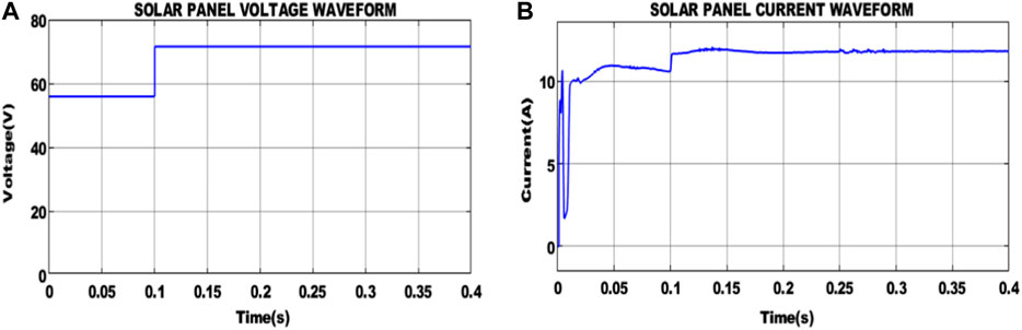
Figure 8. (A) Voltage and (B) current waveforms for the solar panel.

Figure 9 illustrates that the input DC voltage is obtained from the integrated boost-flyback converter. VDC1 and VDC2 with the constant value of 15 V and 16 V, respectively, are maintained. Likewise, Figure 10 shows the DC voltage VDC3 and VDC4 with the stable value of 52 V and 102 V are maintained.

Figure 9

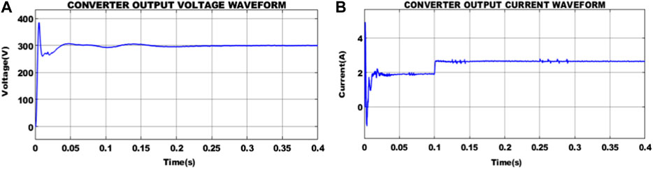
Figure 9. (A) Voltage and (B) current output of IBFC.

Figure 10

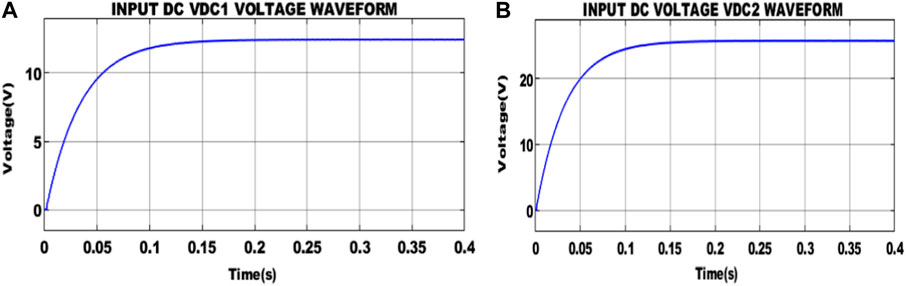
Figure 10. Input (A) VDC1 & (B) VDC2 waveform.

Figure 10 shows the load RMS voltage waveform. From that graph, the load RMS voltage 175 V is accomplished at 0.02s.

From the waveform representation shown in Figure 11, it is noted that a constant voltage of 230 V is supplied to the grid. Similarly, the grid current value of 4 A is maintained.

Figure 11

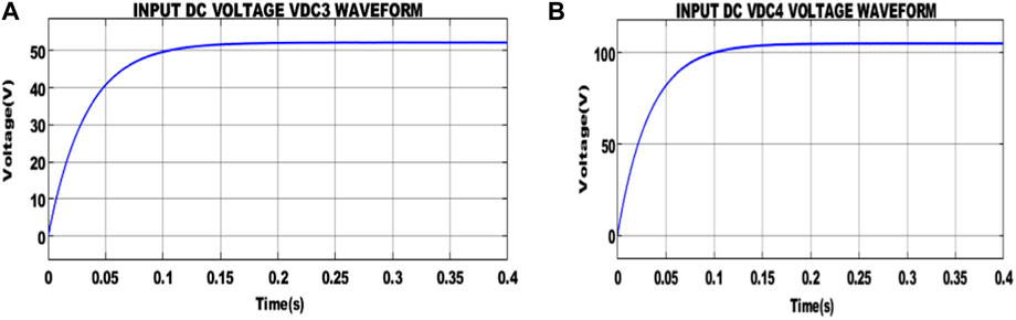
Figure 11. Input (A) VDC3 & (B) VDC4 waveforms.

Figure 12 depicts the waveforms that represent the reactive and real power of grid 1. At 0.03 s, the magnitude of real power stabilizes at 520 W, and the minimized reactive power is achieved.

Figure 12

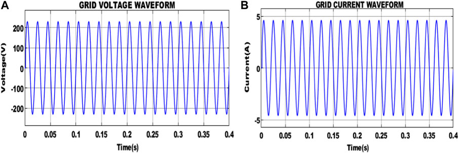
Figure 12. Grids: (A) voltage and (B) current.

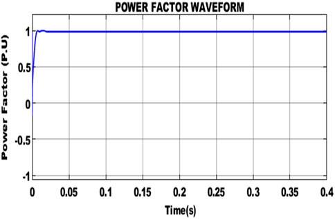
The waveform of the power factor is shown in Figure 13. Thus, a power factor of 1 is attained, denoting that the suggested system operates with efficiency and dependability.

Figure 13

Figure 13. Real and reactive power waveforms.

Figure 14 shows the output current and voltage waveform of the 31-level MLI. Here, the voltage of 220 V is maintained as shown in Figure 14A, and the load current of 4.5 A is achieved, as shown in Figure 14B.

Figure 14

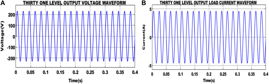
Figure 14. 31-level output (A) voltage and (B) load current waveforms.

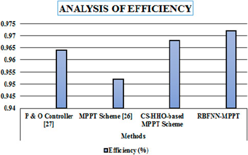
Figure 15 indicates the proposed IBFC converter’s THD value as 2.45%, which has very low harmonics when compared to that of other approaches.

Figure 15

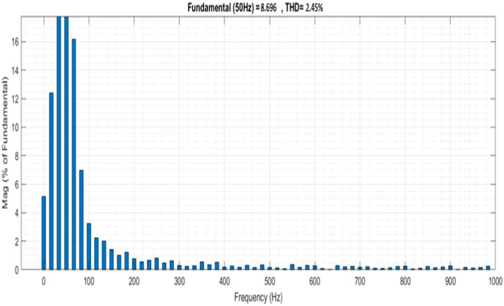
Figure 15. THD waveform.

Table 5 compares several power tracking methods, and Figure 16 shows the corresponding graphs with similar comparisons. As the RBFNN-based MPPT efficiency is 98.80%, Table 5 and Figure 17 demonstrate the various measures, including mean, median, and standard deviation. The considered factors strongly show that the suggested method outperforms the existing methods in terms of the considered factors.

Table 5

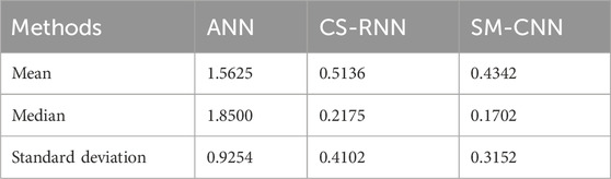
Table 5. Statistical analysis.

Figure 16

Figure 16. Efficiency analysis.

Figure 17

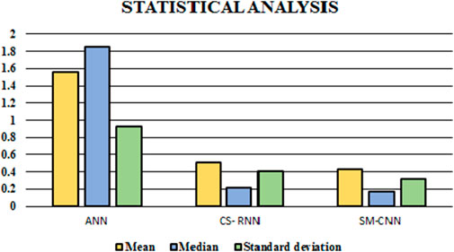
Figure 17. Statistical analysis.

6 Conclusion

We conclude that the proposed system improves high performance to achieve efficiency. The MLIs have been heavily used to improve the PQ of PV systems. The requirement for a large number of components, increased standing voltage, and high harmonic content in the output cause a significant impact on the efficiency of a standard MLI. In this work, a control approach called Spider Monkey Optimization CNN is used with an appropriate level of inverter (31 level) to lessen PQ problems to solve the mitigations. The integrated boost-flyback converter is employed, in order to stabilize the output voltage of the PV panel to achieve the performance. Intended for separating the highest power from the solar PV system, the RBFNN-based MPPT technique is used, and this achieves an efficiency of 97.2%, which is the highest efficiency compared to that of other control methods. The proposed MLI is produced with an enhanced power factor and a lower THD value of 2.45%, and the influence of harmonics is also negligible.

Data availability statement

The original contributions presented in the study are included in the article/Supplementary Material; further inquiries can be directed to the corresponding author.

Author contributions

PA: writing–original draft. SK: writing–original draft.

Funding

The author(s) declare that no financial support was received for the research, authorship, and/or publication of this article.

Conflict of interest

The authors declare that the research was conducted in the absence of any commercial or financial relationships that could be construed as a potential conflict of interest.

Publisher’s note

All claims expressed in this article are solely those of the authors and do not necessarily represent those of their affiliated organizations, or those of the publisher, the editors, and the reviewers. Any product that may be evaluated in this article, or claim that may be made by its manufacturer, is not guaranteed or endorsed by the publisher.

Footnotes

¹For Original Research articles, please note that the Material and Methods section can be placed in any of the following ways: before Results, before or after Discussion.

References

Aarthi, C., Ramya, V. J., Falkowski-Gilski, P., and Divakarachari, P. B. (2023). Balanced spider monkey optimization with Bi-lstm for sustainable air quality prediction. Sustainability 15 (2), 1637. doi:10.3390/su15021637

CrossRef Full Text | Google Scholar

Arjunagi, S., and Patil, N. B. (2021). Optimized convolutional neural network for identification of maize leaf diseases with adaptive ageist spider monkey optimization model. Int. J. Inf. Technol. 15, 877–891. doi:10.1007/s41870-021-00657-3

CrossRef Full Text | Google Scholar

Babu, N., et al. (2020a). An improved adaptive control strategy in grid-tied PV system with active power filter for power quality enhancement. IEEE Syst. J. 15 (2), 2859–2870.

Google Scholar

Babu, N., Guerrero, J. M., Siano, P., Peesapati, R., and Panda, G. (2020b). A novel modified control scheme in grid-tied photovoltaic system for power quality enhancement. IEEE Trans. Industrial Electron. 68 (11), 11100–11110. doi:10.1109/tie.2020.3031529

CrossRef Full Text | Google Scholar

Badoni, M., et al. (2021). Grid tied solar PV system with power quality enhancement using adaptive generalized maximum Versoria criterion. CSEE J. Power Energy Syst.

Google Scholar

Banaei, M. R., Zoleikhaei, A., and Sani, S. G. (2019). Design and implementation of an interleaved switched-capacitor dc-dc converter for energy storage systems. J. Power Technol. 99 (1), 1.

Google Scholar

Bouselham, L., Hajji, M., Hajji, B., and Bouali, H. (2017). A new MPPT-based ANN for photovoltaic system under partial shading conditions. Energy Procedia 111, 924–933. doi:10.1016/j.egypro.2017.03.255

CrossRef Full Text | Google Scholar

Chandra, S., and Gaur, P. (2020). Radial basis function neural network technique for efficient maximum power point tracking in solar photo-voltaic system. Procedia Comput. Sci. 167, 2354–2363. doi:10.1016/j.procs.2020.03.288

CrossRef Full Text | Google Scholar

Chen, Z., Zhou, Q., and Xu, J. (2015). Coupled-inductor boost integrated flyback converter with high-voltage gain and ripple-free input current. IET power Electron. 8 (2), 213–220. doi:10.1049/iet-pel.2014.0066

CrossRef Full Text | Google Scholar

Dhanamjayulu, C., Arunkumar, G., Jaganatha Pandian, B., Ravi Kumar, C. V., Praveen Kumar, M., Rini Ann Jerin, A., et al. (2019). Real-time implementation of a 31-level asymmetrical cascaded multilevel inverter for dynamic loads. IEEE Access 7, 51254–51266. doi:10.1109/access.2019.2909831

CrossRef Full Text | Google Scholar

Golla, M., Chandrasekaran, K., and Simon, S. P. (2021). PV integrated universal active power filter for power quality enhancement and effective power management. Energy Sustain. Dev. 61, 104–117. doi:10.1016/j.esd.2021.01.005

CrossRef Full Text | Google Scholar

Hu, Y., Xiao, W., Cao, W., Ji, B., and Morrow, D. J. (2014). Three-port DC–DC converter for stand-alone photovoltaic systems. IEEE Trans. Power Electron. 30 (6), 3068–3076. doi:10.1109/tpel.2014.2331343

CrossRef Full Text | Google Scholar

Khare, N., Devan, P., Chowdhary, C., Bhattacharya, S., Singh, G., Singh, S., et al. (2020). Smo-dnn: spider monkey optimization and deep neural network hybrid classifier model for intrusion detection. Electronics 9 (4), 692. doi:10.3390/electronics9040692

CrossRef Full Text | Google Scholar

Kumar, A. N., et al. (2018). “A 31-level MLI topology with various level-shift PWM techniques and its comparative analysis,” in 2018 3rd International Conference on Communication and Electronics Systems (ICCES), Coimbatore, India, 15-16 October 2018 (IEEE).

CrossRef Full Text | Google Scholar

Kumar, J. H., Sai Babu, Ch, and Kamalakar Babu, A. (2012). Design and analysis of P&O and IP&O MPPT techniques for photovoltaic system. Berlin, Germany: Springer.

Google Scholar

Lal, J. D., and Thankachan, D. (2021). Statistical evaluation of energy harvesting system models in wireless networks: an empirical perspective.

Google Scholar

Parida, N., Mishra, D., Das, K., Rout, N. K., and Panda, G. (2021). On deep ensemble CNN–SAE based novel agro-market price forecasting. Evol. Intell. 14, 851–862. doi:10.1007/s12065-020-00466-w

CrossRef Full Text | Google Scholar

Pathy, S., et al. (2016). “A modified module integrated—interleaved boost converter for standalone photovoltaic (PV) application,” in 2016 IEEE International Conference on Renewable Energy Research and Applications (ICRERA), Birmingham, United States, 20-23 November 2016 (IEEE).

Google Scholar

Prasad, D., Dhanamjayulu, C., Padmanaban, S., Holm-Nielsen, J. B., Blaabjerg, F., and Khasim, S. R. (2021). Design and implementation of 31-level asymmetrical inverter with reduced components. IEEE Access 9, 22788–22803. doi:10.1109/access.2021.3055368

CrossRef Full Text | Google Scholar

Rajesh, P., Shajin, F. H., and Umasankar, L. (2021). A novel control scheme for PV/WT/FC/battery to power quality enhancement in micro grid system: a hybrid technique. Energy Sources, Part A Recovery, Util. Environ. Eff., 1–17. doi:10.1080/15567036.2021.1943068

CrossRef Full Text | Google Scholar

Ramasamy, S., and Perumal, M. (2021). CNN-based deep learning technique for improved H7 TLI with grid-connected photovoltaic systems. Int. J. Energy Res. 45 (14), 19851–19868. doi:10.1002/er.7030

CrossRef Full Text | Google Scholar

Ray, P., Ray, P. K., and Kumar Dash, S. (2021). Power quality enhancement and power flow analysis of a PV integrated UPQC system in a distribution network. IEEE Trans. Industry Appl. 58 (1), 201–211. doi:10.1109/tia.2021.3131404

CrossRef Full Text | Google Scholar

Ray, P. K., Soumya, R. D., and Mohanty., A. (2018). Fuzzy-controller-designed-PV-based custom power device for power quality enhancement. IEEE Trans. Energy Convers. 34 (1), 405–414. doi:10.1109/tec.2018.2880593

CrossRef Full Text | Google Scholar

Saravanakumar, T., and Saravana kumar, R. (2023). Fuzzy based interleaved step-up converter for electric vehicle. Intelligent Automation Soft Comput. 35, 1103–1118. doi:10.32604/iasc.2023.025511

CrossRef Full Text | Google Scholar

Shen, C.-L., and Chiu, P.-C. (2016). Buck-boost-flyback integrated converter with single switch to achieve high voltage gain for PV or fuel-cell applications. IET Power Electron. 9 (6), 1228–1237. doi:10.1049/iet-pel.2015.0482

CrossRef Full Text | Google Scholar

Shimi, S. L., Thakur, T., Kumar, J., and Chatterji, S. (2013). “MPPT based solar powered cascade multilevel inverter,” in Emerging Research Areas and 2013 International Conference on Microelectronics, Communications and Renewable Energy (AICERA/ICMiCR), Kanjirapally, India, 4-6 June 2013.

CrossRef Full Text | Google Scholar

Shitole, A. B., Sathyan, S., Suryawanshi, H. M., Talapur, G. G., and Chaturvedi, P. (2017). Soft-switched high voltage gain boost-integrated flyback converter interfaced single-phase grid-tied inverter for SPV integration. IEEE Trans. industry Appl. 54 (1), 482–493. doi:10.1109/tia.2017.2752679

CrossRef Full Text | Google Scholar

Spiazzi, G., et al. (2010). “Improved integrated boost-flyback high step-up converter,” in 2010 IEEE International Conference on Industrial Technology, Vina del Mar, Chile, 14-17 March 2010 (IEEE).

CrossRef Full Text | Google Scholar