Modeling of vehicle carbon emissions on horizontal curve road sections

The high carbon emissions of vehicles traveling on horizontal curve road sections cannot be ignored. Facing the difficulty of accurately quantifying the carbon emission of driving on horizontal curves and the unknown causes of high carbon emission, this study proposes to construct a carbon emission prediction model applicable to road sections with different planar geometries. The direct and indirect effects of horizontal curve alignment on vehicle carbon emissions are represented in the model in terms of travel stabilization and speed changes, respectively. A lateral force coefficient parameter was introduced into the model to integrate the carbon emission quantification problem for different planar geometry sections. Meanwhile, field tests were conducted to assess the reliability of the model and the research findings. The model reveals that the geometric parameters of horizontal curves that affect carbon emissions are the radius of the circular curve, the superelevation, and the length of the gentle curve. The root causes of high carbon emissions on horizontal curve road sections are curve driving resistance and speed fluctuations. Under the free-flow driving condition of the highway, the maximum curve radius affecting the carbon emissions of passenger cars and trucks is 400 m and 550 m, respectively. The research results can realize the carbon emission quantification of vehicles on the road sections with different plane geometries. Also, it is helpful to control the high carbon emission of vehicles traveling on horizontal curve road sections.

1 Introduction

The higher carbon emissions typically emitted by vehicles on curved roads have attracted the attention of scholars. Actual road projects have a variety of planar geometries, different values of plane geometry indicators, and varying vehicle speeds (Wang et al., 2019). The mechanisms of these factors on carbon emissions are yet to be explored. If we can accurately assess the quantitative impact of horizontal curve alignment on vehicle carbon emissions, explain the causal mechanism of high carbon emissions from curved roadway travel, and reveal the controllable influencing factors, it will help to mitigate the high carbon emissions caused by road horizontal curve alignment, which will bring long-lasting and significant economic and environmental benefits.

Existing research on vehicle carbon emission prediction has formed a more authoritative database and a mature theoretical framework, including the physical model represented by CMEM (Ataei et al., 2021), and the statistical model represented by MOVES (Lin et al., 2019). Pan et al. (2020) implemented a gradient-enhanced regression tree-based algorithm to predict the carbon emissions of new energy buses on longitudinal slopes section over the fuel cycle. Moradi and Miranda-moreno. (2020) used a support vector regression algorithm to establish a vehicle fuel consumption model parameterized by speed, acceleration, and longitudinal slope gradient. Existing vehicle carbon emission models focus on the high carbon emissions emitted by vehicles traveling uphill, and lack the consideration of the geometric alignment of horizontal curves, thus limiting the accurate prediction of carbon emissions from vehicles traveling on curved roads.

The geometric linearity of horizontal curves is strongly associated with increased vehicle carbon emissions (Ding and Jin, 2018). Vehicle kinematics theory indicates that vehicles are subjected to centrifugal forces when traveling on curved roadways. Given a constant speed, the smaller the radius of the curve, the greater the centrifugal force on the vehicle. Centrifugal forces can affect the vehicle’s lateral stability and driving comfort, and can even cause the driver to slow down before entering a curve (Fitzpatrick et al., 2000). Ko. (2015) used MOVES to model the incremental carbon emissions caused by speed fluctuations of a passenger car on a flat curved roadway. David et al. (2018) obtained a statistical model of vehicle carbon emissions on horizontal curve road sections by regressing measured data with curvature change rate, average speed, and its deviation as parameters. Dong et al. (2019) measured the carbon emission rate of diesel trucks with different curve radius on the highway, concluded that when the radius of the circular curve is greater than 500 m, the vehicle speed is stably close to 100 km/h, and the incremental carbon emission caused by the micro-change of the vehicle speed is very small, and the vehicle carbon emission is almost equal to that of the flat straight road section. Zhang et al. (2019) obtained the carbon emission of a heavy-duty diesel vehicle on a circular curve section without superelevation by conducting real measurements and MOVES simulations on a flat straight road, and pointed out that the carbon emission decreases with the increase of curve radius. The critical curve radius that affects carbon emission is 550 m.

The stability of driving on curved roads affects the driving energy of the vehicle (Zhang et al., 2016), generating corresponding carbon emissions. From the perspective of driving dynamics, the additional cornering resistance of a vehicle, also known as curve driving resistance, is mainly determined by the road surface friction coefficient, wheel angle, and tire load (Peng et al., 2020). The actual horizontal curve road section is usually accompanied by a superelevation, which will reduce the lateral force coefficient of the curved road (Yin et al., 2020). The effect of the installation of superelevation on the curve driving resistance and carbon emissions is currently unknown.

After years of in-depth research, scholars have constructed a clear theoretical framework of vehicle carbon emissions and carried out empirical studies on the high carbon emission patterns of traveling vehicles on curved roads. The results of the study show that the horizontal curve alignment is closely related to vehicle carbon emissions. The direct effect of the horizontal curve line shape on carbon emissions lies in the stability of the vehicle, and the indirect effect lies in the change of operating speed. There is a clear path of research and good progress has been made, however there are still some issues to be resolved. Firstly, there are various plane geometry indicators, which make it more difficult to quantify the carbon emission of vehicles on different plane line conditions. Second, the mechanism of high carbon emissions from traveling on curved roads is not yet clear. These are the challenges that this study is dedicated to solving. As a result, this study is committed to constructing a prediction model of vehicle carbon emissions on horizontal curve sections of roads, and revealing the causal mechanism of high carbon emissions of traveling vehicles on curved roads.

The structure of this manuscript is organized as follows. In section 2, a theoretical model of carbon emission of vehicles traveling on curved roads is constructed, a simplified field test scheme for horizontal curve road sections is derived and proposed, and then field tests are conducted to collect carbon emission data. In section 3, based on the field measurement data, the minimum radius values affecting the carbon emissions of passenger cars and trucks are clarified, and the prediction effectiveness of the vehicle carbon emission model is evaluated. In section 4, a consistent comparison with existing research results is made, and the findings and limitations of the study are briefly summarized. The conclusion section summarizes the research results and their significance.

2 Methods

A combination of theoretical analysis and field trials was used to ensure the reliability of the findings. Specifically, a theoretical model of vehicle carbon emissions on horizontal curve road sections was established through theoretical derivation, revealing the influence mechanism of plane geometry indicators on vehicle carbon emissions. Through the rational design of the field test program, the field test is carried out to measure the carbon emissions of the vehicles on the actual curved roads. Then analyze the change rule of carbon emission of vehicles driving on the curved road. The accuracy of the model prediction is also evaluated with the test data.

2.1 Theoretical modeling of carbon emissions from traveling vehicles on curved roads

The direct effect of road geometry on vehicle carbon emissions lies in the stability of traveling vehicles, and the indirect effect is reflected in the operating speed fluctuation. This study reveals the effect of plane geometry metrics on carbon emissions by analyzing the stability of a vehicle at a constant speed. On the other hand, the carbon emission model of variable-speed traveling on curved roads was developed to reveal the carbon emission rules caused by speed changes under the influence of road alignment.

2.1.1 Direct effect of horizontal curve alignment on vehicle carbon emissions

To ensure the lateral stability and smoothness of traveling, the circular curve will be designed to be superelevated in the lateral direction. On the circular curve segments on the horizontal curve, the superelevation cross slope reaches the full superelevation form. The force analysis of a vehicle is shown in Figure 1. The force balance of the vehicle is as shown in Eq. 1.

$\mathit{F}\mathit{cos}\mathit{\alpha }-\mathit{G}\mathit{sin}\mathit{\alpha }=\mathit{m}\mathit{\mu }(1)$

FIGURE 1

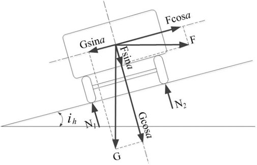
FIGURE 1. Force analysis of a vehicle on a circular curve with an superelevation setting.

The lateral inclination of the roadway is generally small, and $\sin \mathrm{\alpha }\approx \tan \mathrm{\alpha }={\mathrm{i}}_{\mathrm{h}}$, $\cos \mathrm{\alpha }=1$. where ${\mathrm{i}}_{\mathrm{h}}$ is the value of superelevation. The lateral force coefficient can be calculated from Eq. 2 on circular curved roadway sections with superelevation (AASHTO, 2011).

$\mathit{\mu }=\frac{{\mathit{V}}^{\mathbf{2}}}{\mathit{g}\mathit{R}}-{\mathit{i}}_{\mathit{h}}(2)$

Setting the superelevation on the circular curve can offset all or part of the centrifugal force, and the remaining centrifugal force is balanced by the side deflection force acting on the front and rear tires, and the total side deflection force acting on the tires can be calculated by Eq. 3.

${\mathit{F}}_{\mathit{L}}=\mathit{m}\mathit{g}\mathit{\mu }=\frac{\mathit{m}{\mathit{V}}^{\mathbf{2}}}{\mathit{R}}-\mathit{m}\mathit{g}{\mathit{i}}_{\mathit{h}}(3)$

A tire produces a lateral deflection angle under the action of a lateral deflection force. For the force on a single tire, the cornering stiffness ${\mathit{C}}_{\mathit{a}}$ is usually used to characterize the lateral deflection force corresponding to a 1 rad lateral deflection angle, which reflects the deformation characteristics of the tire (You and Jeong, 2002), as shown in Eq. 4.

${\mathit{F}}_{\mathit{L}}={\mathit{C}}_{\mathit{a}}\partial (4)$

where ${\mathit{C}}_{\mathit{a}}$ represents tire cornering stiffness (kN/rad). $\partial$ refers to the tire side deflection angle (rad).

When the vehicle is accurately steered, the centrifugal acceleration is less than 0.4 g, the tire turning stiffness can be regarded as a constant, and the side deflection force and side deflection angle have a linear positive correlation with the turning stiffness as a scaling factor. In this case, the side deflection force is in the range of 0–2000 N and the side deflection angle is less than 3°. (Mitschke and Wallentowitz, 2014).

${\mathit{F}}_{\mathit{y}\mathit{f}}=\frac{\left(\mathit{m}{\mathit{V}}^{\mathbf{2}}/\mathit{R}-\mathit{m}\mathit{g}{\mathit{i}}_{\mathit{h}}\right){\mathit{L}}_{\mathit{r}}}{\mathit{L}}(5)$

${\mathit{F}}_{\mathit{y}\mathit{r}}=\frac{\left(\mathit{m}{\mathit{V}}^{\mathbf{2}}/\mathit{R}-\mathit{m}\mathit{g}{\mathit{i}}_{\mathit{h}}\right){\mathit{L}}_{\mathit{f}}}{\mathit{L}}(6)$

The problem of stability of a vehicle traveling on a curved road is determined by the lateral dynamic characteristics. In the vehicle monorail model shown in Figure 2, the dynamic response of the vehicle is Eq. 7.

$\left\{\begin{array}{l}\mathit{m}\mathit{V}\left(\dot{\mathit{\beta }}+\dot{\mathit{\phi }}\right)\mathit{sin}\mathit{\beta }-\mathit{m}\dot{\mathit{V}}\mathit{cos}\mathit{\beta }+{\mathit{F}}_{\mathit{x}\mathit{r}}+{\mathit{F}}_{\mathit{x}\mathit{f}}\mathit{cos}\mathit{\delta }-{\mathit{F}}_{\mathit{y}\mathit{f}}\mathit{sin}\mathit{\delta }-{\mathit{F}}_{\mathit{r}}-{\mathit{F}}_{\mathit{a}}=\mathbf{0}\\ \mathit{m}\mathit{V}\left(\dot{\mathit{\beta }}+\dot{\mathit{\phi }}\right)\mathit{cos}\mathit{\beta }+\mathit{m}\dot{\mathit{V}}\mathit{sin}\mathit{\beta }-{\mathit{F}}_{\mathit{y}\mathit{r}}-{\mathit{F}}_{\mathit{x}\mathit{f}}\mathit{sin}\mathit{\delta }-{\mathit{F}}_{\mathit{y}\mathit{f}}\mathit{cos}\mathit{\delta }-\mathit{m}\mathit{g}{\mathit{i}}_{\mathit{h}}=\mathbf{0}\\ {\mathit{I}}_{\mathit{Z}}\ddot{\mathit{\phi }}-\left({\mathit{F}}_{\mathit{x}\mathit{f}}\mathit{sin}\mathit{\delta }-{\mathit{F}}_{\mathit{y}\mathit{f}}\mathit{cos}\mathit{\delta }\right){\mathit{L}}_{\mathit{f}}+{\mathit{F}}_{\mathit{y}\mathit{r}}{\mathit{L}}_{\mathit{r}}=\mathbf{0}\end{array}\right.(7)$

where ${\mathit{F}}_{\mathit{i}\mathit{i}}$ (ii = xf, yf) is the fraction of the front wheel drive force in the X and Y-axes directions (N). ${\mathit{F}}_{\mathit{j}\mathit{j}}$ (jj = xr,yr) indicates the rear wheel drive force components in the X and Y-axes directions (N). $\mathrm{\delta }$ is the front wheel steering angle (°). $\mathrm{\beta }$ indicates the lateral deflection angle at the center of mass (°). $\mathrm{\phi }$ is the traverse angle (°). ${\mathit{L}}_{\mathit{f}}$ indicates the front wheelb’ase (m). L_r is the rear wheelbase (m).

FIGURE 2

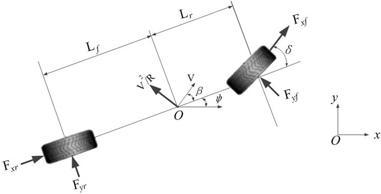
FIGURE 2. Vehicle monorail model.

When the vehicle is accurately steered, $\dot{\mathrm{\beta }}=0,\dot{\mathrm{\phi }}=0$. Assuming that the front wheel angle of rotation and the lateral deflection angle at the center of mass are small, their cosines are approximately 1 and their multiplication is approximately 0. Derivation of Eq. 7 leads to the combined force exerted by the vehicle in the longitudinal direction shown in Eq. 8.

${\mathit{F}}_{\mathit{x}\mathit{f}}+{\mathit{F}}_{\mathit{x}\mathit{r}}={\mathit{F}}_{\mathit{r}}+{\mathit{F}}_{\mathit{a}}-\left(\mathit{m}\mathit{v}\dot{\mathit{\phi }}-\mathit{m}\mathit{g}{\mathit{i}}_{\mathit{h}}\right)\left(\mathit{sin}\mathit{\beta }-\frac{{\mathit{L}}_{\mathit{f}}}{\mathit{L}}\mathit{sin}\mathit{\delta }\right)(8)$

$\mathit{sin}\mathit{\beta }=\frac{{\mathit{L}}_{\mathit{r}}}{\mathit{L}}\mathit{sin}\mathit{\delta }-\frac{{\mathit{L}}_{\mathit{r}}}{\mathit{L}}\mathit{sin}{\partial }_{\mathit{f}}-\frac{{\mathit{L}}_{\mathit{f}}}{\mathit{L}}\mathit{sin}{\partial }_{\mathit{r}}(9)$

where $\partial \mathrm{f}$, $\partial \mathrm{r}$ indicate the lateral deflection angle of the front and rear axles (°). L indicates the wheelbase(m).

When the vehicle is accurately steered, the load is uniformly distributed on the four tires, the turning stiffness and side deflection angle of the tires are equal (Wong, 2008), and the specific characteristic conditions are shown in Eq. 10 and Eq. 11, Eq. 12 and Eq. 13.

${\mathit{L}}_{\mathit{f}}={\mathit{L}}_{\mathit{r}}(10)$

${\mathit{C}}_{\mathit{a}\mathit{f}}={\mathit{C}}_{\mathit{a}\mathit{r}}={\mathit{C}}_{\mathit{a}}(11)$

$\partial \mathit{f}=\partial \mathit{r}=\partial (12)$

${\mathit{C}}_{\mathit{a}\mathit{v}}=\mathit{n}{\mathit{C}}_{\mathit{a}}(13)$

Combining Eq. 9–14 can be obtained.

$\mathit{sin}\mathit{\beta }=\frac{{\mathit{L}}_{\mathit{r}}}{\mathit{L}}\mathit{sin}\mathit{\delta }-\mathit{sin}\partial (14)$

Substituting Eq. 14 into Eq. 8 leads to Eq. 15.

${\mathit{F}}_{\mathit{x}\mathit{f}}+{\mathit{F}}_{\mathit{x}\mathit{r}}={\mathit{F}}_{\mathit{r}}+{\mathit{F}}_{\mathit{a}}+\left({\frac{\mathit{m}\mathit{V}}{\mathit{R}}}^{\mathbf{2}}-\mathit{m}\mathit{g}{\mathit{i}}_{\mathit{h}}\right)\mathit{sin}\partial (15)$

The curve driving resistance, F_k, can be obtained as shown in Eq. 16.

${\mathit{F}}_{\mathit{k}}=\left({\frac{\mathit{m}\mathit{V}}{\mathit{R}}}^{\mathbf{2}}-\mathit{m}\mathit{g}{\mathit{i}}_{\mathit{h}}\right)\mathit{sin}\partial (16)$

Based on the linear characteristics of the turning stiffness, the curve driving resistance and the curve driving resistance work done by the vehicle in the circular curve section where the superelevation is set up can be expressed by Equation. 17 and Equation. 18.

${\mathit{F}}_{\mathit{k}}=\frac{{\left(\mathit{m}{\mathit{V}}^{\mathbf{2}}/\mathit{R}-\mathit{m}\mathit{g}{\mathit{i}}_{\mathit{h}}\right)}^{\mathbf{2}}}{\mathit{n}\mathit{C}\mathit{a}}(17)$

${\mathit{W}}_{\mathit{k}}=\frac{{\left(\mathit{m}{\mathit{V}}^{\mathbf{2}}/\mathit{R}-\mathit{m}\mathit{g}{\mathit{i}}_{\mathit{h}}\right)}^{\mathbf{2}}}{\mathit{n}\mathit{C}\mathit{a}}{\mathit{S}}_{\mathit{k}}(18)$

where W_k represents the work done by the curve driving resistance(N m). S_k denotes trip mileage (m). n indicates the number of tires.

Due to its high load attributes, trucks are usually equipped with a non-independent suspension system to increase the load-carrying capacity and to avoid large side deflection angles of the tires during cornering operation. Non-independent suspension systems cause the left and right wheels to interact with each other, which generates suspension resistance and depletes part of the vehicle’s mechanical energy (Wong, 2008). The independent suspension system used in passenger cars does not have this part of the energy consumption. The energy consumption induced by a truck turning on a curved road is determined by the curve driving resistance and the suspension resistance, as shown in Eq. 19.

${\mathit{W}}_{\mathit{k}}=\left[\frac{{\left(\mathit{m}{\mathit{V}}^{\mathbf{2}}/\mathit{R}-\mathit{m}\mathit{g}{\mathit{i}}_{\mathit{h}}\right)}^{\mathbf{2}}}{\mathit{n}\mathit{C}\mathit{a}}+{\mathit{F}}_{\mathit{t}\mathit{c}}\right]{\mathit{S}}_{\mathit{k}}(19)$

where ${\mathit{F}}_{\text{tc}}$ indicates the suspension resistance due to the mass on the spring(N).

When the vehicle is traveling at a uniform speed in a circular curve section with superelevation, the carbon emission model is shown in Eq. 20. It shows that in the section of circular curves with superelevation, the plane geometry indicators that have an impact on vehicle carbon emissions include curve radius and superelevation. The mechanical characteristic parameter that has an impact on vehicle carbon emissions is the lateral force coefficient.

$\mathit{C}{\mathit{O}}_{\mathbf{2}}=\left({\mathit{W}}_{\mathit{r}}+{\mathit{W}}_{\mathit{a}}+{\mathit{W}}_{\mathit{k}}\right){\mathit{n}}_{\mathit{c}\mathit{o}\mathbf{2}}+{\mathit{C}}_{\mathbf{0}}+{\mathit{C}}_{\mathit{T}}(20)$

where W_r and W_a represents the work done by rolling resistance and air resistance, respectively (N m). C₀ and C_T represent carbon emissions (kg) from idle fuel consumption and carbon emissions from diesel exhaust cleaning, respectively, and the calculation methods are detailed in the authors’ previous research literature (Dong et al., 2020). n_co2 is the conversion factor between the driving energy and the carbon emission. Based on the positive correlation between the energy and carbon emissions of vehicle fuels, the authors’ previous research literature (Dong et al., 2023) used the IPCC. (2006) to obtain carbon emission rates of 0.296 kgCO₂/MJ and 0.213 kgCO₂/MJ for gasoline and diesel engines, respectively.

In particular, from Eq. 17, the curve driving resistance for a circular curve section without superelevation is shown in Eq. 21. This directly reveals the direct effect of curve radius on carbon emissions, where the curve driving resistance is proportional to the square of the centrifugal acceleration, proportional to the fourth power of the vehicle speed, and proportional to the square of the lateral deflection angle, as shown in Eq. 22 and Eq. 23. The longitudinal speed of the tire is equivalent to the traveling speed, and the lateral acceleration of the tire is approximately equal to the centrifugal acceleration of the vehicle.

${\mathit{F}}_{\mathit{k}}={\mathit{F}}_{\mathit{L}}\mathit{\alpha }=\frac{\mathit{m}{\mathit{V}}^{\mathbf{2}}\mathit{\alpha }}{\mathit{R}}=\frac{{\mathit{m}}^{\mathbf{2}}{\mathit{V}}^{\mathbf{4}}}{\mathbf{4}{\mathit{C}}_{\mathit{a}}{\mathit{R}}^{\mathbf{2}}}(21)$

${\mathit{F}}_{\mathit{k}}\propto {\left(\frac{{\mathit{V}}^{\mathbf{2}}}{\mathit{R}\mathit{g}}\right)}^{\mathbf{2}}(22)$

${\mathit{F}}_{\mathit{k}}\propto {\mathit{\alpha }}^{\mathbf{2}}(23)$

When the passenger car maintains a uniform speed on a circular curve road section, the work done by the curve driving resistance is shown in Eq. 24. The incremental carbon emission caused by the curve driving resistance is called the vehicle turning carbon emissions. It is inversely proportional to the square of the curve radius and proportional to the fourth power of the speed.

${\mathit{W}}_{\mathit{k}}=\frac{{\mathit{m}}^{\mathbf{2}}{\mathit{V}}^{\mathbf{4}}}{\mathbf{4}{\mathit{C}}_{\mathit{a}}{\mathit{R}}^{\mathbf{2}}}{\mathit{S}}_{\mathit{k}}(24)$

2.1.2 Indirect effects of horizontal curve alignment on vehicle carbon emissions

The indirect effect of horizontal curve alignment on vehicle carbon emissions is reflected in changes in operating speed. Vehicles traveling on flat curve roads with small radius usually exhibit significant speed fluctuations (Bonneson and Pratt, 2009; Wen and Eric, 2010). As the radius of the circular curve gets larger, the operating speed of the vehicle on the flat curve section gradually tends to stabilize, and the difference between the entry speed and the speed at the midpoint of the curve gradually decreases (Paolo, 2018). The greater the change in vehicle speed, the greater the inertial resistance, which will cause a change in carbon emissions.

When the vehicle drives through the curve with variable speed, the resistance along the direction of the traveling trajectory includes rolling resistance, air resistance, inertia resistance, and curve driving resistance. By integrating Eq. 18 and Eq. 24 in the travel time, the curve driving resistance can be obtained for the vehicle traveling at variable speed. The work done by the curve driving resistance of a passenger car traveling at variable speed on a circular curve section and a transition curve section are Eq. 25 and Eq. 26, respectively. For trucks, these are Eq. 27 and Eq. 28, respectively.

${\mathit{W}}_{\mathit{k}-\mathbf{Circular}-\mathbf{car}}={\displaystyle \underset{\mathbf{0}}{\overset{\mathit{t}}{\int }}}\frac{{\left[\mathit{m}\mathit{V}{\left(\mathit{t}\right)}^{\mathbf{2}}/\mathit{R}-\mathit{m}\mathit{g}{\mathit{i}}_{\mathit{h}}\right]}^{\mathbf{2}}}{\mathbf{4}{\mathit{C}}_{\mathit{a}}}\mathit{d}{\mathit{S}}_{\mathit{k}}\left(\mathit{t}\right)(25)$

${\mathit{W}}_{\mathit{k}-\mathbf{Transition}-\mathbf{car}}={\displaystyle \underset{\mathbf{0}}{\overset{\mathit{t}}{\int }}}\frac{{\left[\mathit{m}\mathit{V}{\left(\mathit{t}\right)}^{\mathbf{2}}/\mathit{R}\left(\mathit{t}\right)-\mathit{m}\mathit{g}{\mathit{i}}_{\mathit{h}}\left(\mathit{t}\right)\right]}^{\mathbf{2}}}{\mathbf{4}{\mathit{C}}_{\mathit{a}}}\mathit{d}{\mathit{S}}_{\mathit{k}}\left(\mathit{t}\right)(26)$

${\mathit{W}}_{\mathit{k}-\mathbf{Circular}-\mathbf{truck}}={\displaystyle \underset{\mathbf{0}}{\overset{\mathit{t}}{\int }}}\frac{{\left[\mathit{m}\mathit{V}{\left(\mathit{t}\right)}^{\mathbf{2}}/\mathit{R}-\mathit{m}\mathit{g}{\mathit{i}}_{\mathit{h}}\right]}^{\mathbf{2}}}{\mathit{n}{\mathit{C}}_{\mathit{a}}}\mathit{d}{\mathit{S}}_{\mathit{k}}\left(\mathit{t}\right)+{\mathit{F}}_{\mathit{t}\mathit{c}}{\mathit{S}}_{\mathit{k}}(27)$

${\mathit{W}}_{\mathit{k}-\mathbf{Transition}-\mathbf{truck}}={\displaystyle \underset{\mathbf{0}}{\overset{\mathit{t}}{\int }}}\left\{\frac{{\left[\mathit{m}\mathit{V}{\left(\mathit{t}\right)}^{\mathbf{2}}/\mathit{R}\left(\mathit{t}\right)-\mathit{m}\mathit{g}{\mathit{i}}_{\mathit{h}}\left(\mathit{t}\right)\right]}^{\mathbf{2}}}{\mathit{n}{\mathit{C}}_{\mathit{a}}}+{\mathit{F}}_{\mathit{t}\mathit{c}}\left(\mathit{t}\right)\right\}\mathit{d}{\mathit{S}}_{\mathit{k}}\left(\mathit{t}\right)(28)$

Based on the power load of the vehicle traveling at variable speed on the horizontal curve roadway, the vehicle carbon emission model can be obtained as shown in Eq. 29.

$\mathit{C}{\mathit{O}}_{\mathbf{2}}=\left({\mathit{W}}_{\mathit{r}}+{\mathit{W}}_{\mathit{a}}+{\mathit{W}}_{\mathit{k}}+{\mathit{W}}_{\mathit{e}}+{{\mathit{W}}_{\mathit{t}}}^{\prime }+{\mathit{Q}}_{\mathit{h}}\right){\mathit{n}}_{\mathit{c}\mathit{o}\mathbf{2}}+{\mathit{C}}_{\mathbf{0}}+{\mathit{C}}_{\mathit{T}}(29)$

where $W_k$ is equal to the integral of the curve driving resistance over the traveling time. W_e represents the work done by inertial resistance (N m). ${W_t}^{\prime }$ denotes the work done by the engine counter drag force at idle coasting (N m). ${\mathit{Q}}_{\mathit{h}}$ indicates the mechanical energy consumed by the braking force (N m) (Dong et al., 2023).

Compared with the vehicle carbon emission model for a flat curved road section at uniform speed, the variable speed model takes into account the fact of the curve driving resistance. The curve driving resistance during travel varies with speed. The variable speed model takes into account the work done by the inertial drag during acceleration and deceleration, the work done by the engine counter-drag during idling, and the braking loss energy during braking.

In terms of driving resistance distribution, speed change affects vehicle carbon emissions in three ways, specifically, i.e., speed change not only generates inertial resistance, affects rolling resistance and air resistance, but also affects the curve driving resistance.

2.2 Measurement of carbon emissions from curve-driving

Given that the direct effect of road geometry on vehicle carbon emissions lies in the stability of driving, and the indirect effect is reflected in the change of operating speed, this study proposes to carry out uniform speed driving and variable speed driving tests respectively. Specifically, the test vehicle is required to drive at a constant speed to measure the carbon emissions caused by the driving stability of curved roads. Then, the field road following test is carried out to reveal the changes in the carbon emissions caused by changes in the driving speed of curved roads.

2.2.1 Field trial design

The road plane linear conditions and speed determine the carbon emissions. From the perspective of vehicle dynamics, the lateral force can be regarded as an intermediate parameter for the influence of these factors on carbon emission. Vehicle carbon emission modeling under different plane linear conditions can be regarded as a relationship model between lateral force coefficients and carbon emissions. Such a treatment can simplify the analysis of the combined effects of different plane geometry indicators on carbon emissions, while ensuring the reliability of the research findings.

For passenger cars, the work done by the curve driving resistance on the circular curve and transition curve sections is shown in Eq. 30 and Eq. 31, respectively, which is characterized by the lateral force coefficient as the dependent variable. For trucks, it is Eq. 32 and Eq. (33).

${\mathit{W}}_{\mathit{k}-\mathbf{Circular}-\mathbf{car}}=\frac{{\mathit{m}}^{\mathbf{2}}{\mathit{g}}^{\mathbf{2}}{\mathit{\mu }}^{\mathbf{2}}}{\mathbf{4}{\mathit{C}}_{\mathit{a}}}{\mathit{S}}_{\mathit{k}}(30)$

${\mathit{W}}_{\mathit{k}-\mathbf{Transition}-\mathbf{car}}={\displaystyle \underset{\mathbf{0}}{\overset{\mathit{t}}{\int }}}\frac{{\mathit{m}}^{\mathbf{2}}{\mathit{g}}^{\mathbf{2}}\mathit{\mu }{\left(\mathit{t}\right)}^{\mathbf{2}}}{\mathbf{4}{\mathit{C}}_{\mathit{a}}}\mathit{d}{\mathit{S}}_{\mathit{k}}\left(\mathit{t}\right)(31)$

${\mathit{W}}_{\mathit{k}-\mathbf{Circular}-\mathbf{truck}}=\frac{{\mathit{m}}^{\mathbf{2}}{\mathit{g}}^{\mathbf{2}}{\mathit{\mu }}^{\mathbf{2}}}{\mathit{n}{\mathit{C}}_{\mathit{a}}}{\mathit{S}}_{\mathit{k}}+{\mathit{F}}_{\mathit{t}\mathit{c}}{\mathit{S}}_{\mathit{k}}(32)$

${\mathit{W}}_{\mathit{k}-\mathbf{Transition}-\mathbf{truck}}={\displaystyle \underset{\mathbf{0}}{\overset{\mathit{t}}{\int }}}\left[\frac{{\mathit{m}}^{\mathbf{2}}{\mathit{g}}^{\mathbf{2}}\mathit{\mu }{\left(\mathit{t}\right)}^{\mathbf{2}}}{\mathit{n}{\mathit{C}}_{\mathit{a}}}+{\mathit{F}}_{\mathit{t}\mathit{c}}\left(\mathit{t}\right)\right]\mathit{d}{\mathit{S}}_{\mathit{k}}\left(\mathit{t}\right)(33)$

This in turn allows for field tests to be conducted using the lateral force coefficient as the dependent variable to validate the accuracy of the model. The intermediate parameter of the transverse force coefficient was adopted as a control variable during the test, avoiding the effects of multiple factors on carbon emissions. Experimenting with this way would simplify to a greater extent the assessment of field test data for carbon emission modeling and avoid the complexity and redundancy of the experiment.

For the specific relationship between the lateral force coefficient and carbon emission, there is no authoritative research result for clear reference. How to explore the change of transverse force of actual traveling on a circular curve roadway, and the carbon emission rules under the condition of transverse force? To address this question, conducting a field test is an essential key link. In this experiment, a circular curve of different radii was measured at a flat automobile test track to measure the lateral force coefficients and carbon emissions under different radii of the circular curve. After evaluating the reliability of the carbon emission model for the circular curve section without superelevation, a few data are taken to further validate the carbon emission model for the circular curve section under different superelevation conditions. This test program can not only gradually verify the carbon emission model under different plane line conditions, but also ensure the reliability of the test results and research findings.

Vehicles in a small radius curve, tend to drive at low speeds, resulting in high lateral force coefficients, and there is a general acceleration and deceleration behavior. As the radius increases, the speed gradually increases, which is more favorable for driving stability. The coefficient of lateral force decreases gradually and the speed stabilizes after going from 0.4 to 0.15. The radius, if increased to infinity, the lateral force coefficients become smaller to zero value. Scholars have been obtained through field tests, when the radius is greater than 550 m, the speed is stable and tends to 100 km/h (Cruz et al., 2017). The existing literature on the speed variation rule presents two ideas that can be used to guide the design of the carbon emission test in this manuscript. Specifically, the magnitude of the lateral force coefficient affects the acceleration and deceleration speeds of a vehicle on a circular curve section, which determines the maximum curve radius that affects carbon emissions. The carbon emission increment caused by the acceleration and deceleration can be obtained by calculating the carbon emission difference between the conditions of normal driving on the circular curve roadway, and uniform speed driving on the flat straight roadway. The value of uniform speed is the speed at the midpoint position of the curve. The carbon emission under the condition of uniform speed can be predicted based on the model constructed by the author’s previous research (Xu et al., 2020). Secondly, the vehicle turning carbon emissions can be obtained by finding the difference of carbon emissions from the vehicle uniform speed operation test on the circular curve and the flat and straight road sections.

Based on the above analysis, the field trial program was designed as follows.

At a flat automobile test site, a circular curve without over-height is placed on site as a test section. The field test was divided into two parts, namely, normal driving and uniform speed driving tests. The normal driving test uses radius as a control parameter to capture carbon emissions, aiming to determine the minimum radius value of the circular curve that does not affect carbon emissions. The speed value is the operating speed at the midpoint of the curve as measured in a normal driving test. The normal driving test requires one group of drivers to drive normally on circular curve sections. The uniform driving test requires another group of drivers to drive uniformly at the target speed in circular curve sections and flat straight sections. Under the condition of the same vehicle speed, the difference in carbon emission between the uniform speed driving test on the circular curve section and the uniform speed driving test on the flat section is the vehicle turning carbon emissions caused by the curve driving resistance. The difference in carbon emissions between normal and constant speed driving tests on the circular curve section under the condition of the same radius is the carbon emission caused by speed fluctuations.

The results of carbon emission tests on circular curved sections carried out at the automobile test site can reveal the carbon emission rules of vehicles with different lateral force coefficients. By integrating Eq. 2 and, Eq. 18 Eq. 19, it can be inferred that when the value of the lateral force system is constant, the carbon emission prediction results are consistent regardless of the change in the plane linear condition. This result clarifies the reliability of the prediction model from the theoretical point of view for the circular curve section with superelevation settings, and the transition curve section. In addition, this manuscript also evaluates the accuracy of the model predictions from an empirical perspective. The test sections were selected to be a gently sloping circular curve section of the Xi-Han Expressway with a superelevation setting. A gently curved section of the roadway was designed and sampled at the automotive proving grounds. The transition curve sections were designed and routed at the automotive proving grounds.

The transition curve test sections were set up on the automobile test site. The test results were used to assess the accuracy of vehicle carbon emission predictions for transitional curve sections without excessive superelevation. The theoretical model shows that for both circular and transition curves, the lateral force coefficient can be regarded as a mechanically characterized parameter that affects vehicle carbon emissions. The lateral force coefficients have the same effect on vehicle carbon emissions for both circular curve sections and transition curve road sections. At the same time, the transition curve can be regarded as a circular curve section with gradual changes in curvature and superelevation. If the carbon emission prediction accuracy of the circular curve section with superelevation reaches a high level, it can be equated with the same prediction accuracy of the carbon emission on the transition curve section.

Test data from vehicles traveling normally on a circular curve section at the automobile test site were used to assess the reliability of the carbon emission model for vehicles traveling on the circular curve sections under variable speed conditions.

2.2.2 Field test methodology

To clarify the minimum radius of the curve that does not affect the carbon emissions of passenger cars and trucks respectively, this test focuses on the test section of the curve with a radius between 100 m and 600 m. The results of the field test are compared with the carbon emissions of vehicles on flat straight road sections to determine the minimum radius of the circular curve that affects carbon emissions. The circular curve and flat straight test sections were measured at the automobile test site. There are 13 circular curve test sections with radii of 100 m, 150 m, 200 m, 250 m, 300 m, 350 m, 400 m, 450 m, 500 m, 550 m, 600 m, 800 m, and 1500 m respectively. In the normal driving test of the circular curve section, the speeds at the beginning and end points of the circular curve and the midpoint of the curve need to be recorded, and the carbon emission is accounted for based on the instantaneous fuel consumption. In a uniform speed test on circular curve sections, the carbon emissions of a specified speed at a uniform speed need to be measured.

In the selected circular curve test section of Xibao Expressway, one group of drivers was asked to drive at a certain speed and the other group of drivers was asked to drive normally.

For the carbon emission tests under two different driving conditions, namely, constant speed and variable speed, it is strictly controlled that the two groups of drivers should not be exchanged with each other. The tests all collected at least 40 sets of valid fuel consumption data to ensure the reliability of the carbon emission modeling assessment conducted subsequently. To facilitate the comparison of the carbon emissions of different driving distances, the carbon emission rate of 100 km was used to characterize the carbon emissions of the vehicle.

(1) Test vehicles

Two types of passenger cars and three types of trucks are selected as typical vehicles, which are referenced from the results of the authors’ survey (Dong et al., 2023) on the proportion of vehicle types in China’s highway traffic volume in recent years. The two passenger cars are a small sedan, represented by the Chevrolet McLaren, and an urban crossover, represented by the Chevrolet Copacetic, hereafter denoted by Car I Car II, respectively. The three trucks are Dongfeng medium truck, Jiefang heavy-duty truck, and Jiefang tractor, which are denoted as Truck I, Truck II, and Truck III, respectively, in the following. The test vehicles were categorized into two vehicle types: passenger cars and trucks, taking into account the differences in operating speeds and lateral force coefficients between passenger cars and trucks on horizontal curve sections.

(2) Test road sections

To measure the direct effect of road plane alignment on vehicle carbon emissions and exclude the effect of route longitudinal section alignment on carbon emissions, the Chang’an University automobile test site was chosen as the test site. By measuring and setting up 13 circular curve test sections in the automobile test site, the radii of the circular curves are 100 m, 150 m, 200 m, 250 m, 300 m, 350 m, 400 m, 450 m, 500 m, 550 m, 600 m, 800 m, and 1500 m, respectively, and the automobile test site is a flat cement concrete pavement, the longitudinal slopes slope ranges from −1∼1%, and there is no set road cross slope. Due to the site size limitation, the size of the radius of the circular curves was changed by changing the size of the radius of the circular curves one by one to measure the carbon emission of the vehicles under different radii of the circular curves. The route and inner and outer edges of the test section were placed and positioned using a total station.

The geometrical lines of the test sections, which are circular and transition curve, are obtained by sampling at the automobile test site. The design indicators for the transition curve sections are shown in Table 1.

TABLE 1

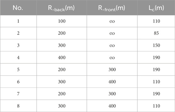
TABLE 1. Design details for transition curve sections.

Considering that the actual curved roads are set with superelevation, six circular curved sections with superelevation were selected as test road sections on the Xi-Han Freeway. The design indicators for the selected test sections are shown in Table 2.

(3) Test instruments

TABLE 2

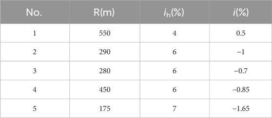
TABLE 2. Design details for circular curve sections with superelevation setting.

The instruments selected for this test are as follows: Portable Automobile USB E-CAN Measuring Instrument, JDSZ-EP-1-1D Vehicle-mounted Diesel Fuel Consumption Measuring Instrument, Laptop Computer, Total Station Instrument, Sigma Split Anemometer AS8336, Digital Camera and Crash Bucket.

(4) Motorists

In the normal driving test, the driver is required to drive normally and is not allowed to drive aggressively to obtain the value of the maximum radius of the curve that affects the speed of the vehicle. The constant speed test requires the driver to drive at different speeds to obtain the additional carbon emissions of the vehicle as determined by different lateral force coefficients.

3 Results

The field test data can be used to analyze the carbon emission rules of vehicles on horizontal curve road sections, and also to assess the reliability of the carbon emission model for vehicles on horizontal curve road sections.

3.1 Minimum radius affecting vehicle carbon emissions

The speed change curve of the test vehicle under normal driving conditions on the circular curve section is shown in Figure 3. Characteristic points 1, 2, and 3 in the figure indicate the starting point, midpoint, and end position of the circular curve test road, respectively.

FIGURE 3

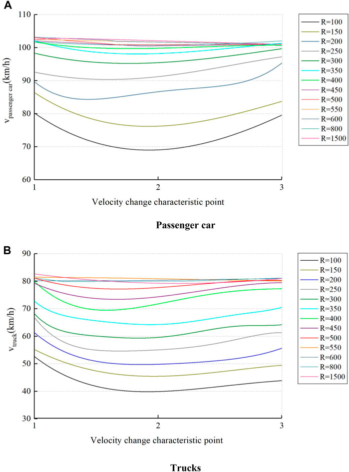
FIGURE 3. Vehicle velocity profile on the circular curve section. (A) speed profile of passenger cars. (B) speed profile of trucks.

In Figure 3, when the radius of the curve is larger than a certain value, the operating speed shows a “U-shaped” trend. The vehicle will take certain deceleration behavior before entering the curve, and after passing the midpoint of the curve, the vehicle continuously accelerates out of the curve. For the same radius of the curve section, the vehicle enters the curve after the maximum deceleration. The smaller the radius, the more obvious the change in running speed. In addition, the smaller the radius, the lower the running speed at the midpoint of the curve; the larger the radius, the higher the running speed at the midpoint of the curve. As the radius increases, the lateral force coefficient decreases. For the passenger car, when the curve radius is 100 m, the speed is low, and the transverse force coefficient u is close to 0.4; with the increment of the radius, the speed increases gradually, and the transverse force coefficient decreases gradually; until the radius is 400 m, the speed reaches 100 km/h, and the transverse force coefficient is 0.15. This running speed law is similar to that of the measured results of Russo et al. (2016) and Sil et al. (2019); while the transverse force variation law is in general agreement with the measured results of Bonneson. (2000), who conducted the transverse force coefficient test on dry pavements of U.S. highways. For the truck, when the radius of the circular curve is greater than or equal to 550 m, the vehicle speed tends to be stabilized and reaches 80 km/h. This is consistent with the measured results of Cruz et al. (2017). This shows that the basic data of vehicle operating speed measured in this test has a certain degree of reliability, which can reflect the change rule of speed and lateral force of actual traveling under different radii. Vehicle carbon emission data obtained under the conditions of this law are also reliable, and the test results are shown in Figure 4. Among them, V-middle is used to indicate the vehicle speed at the midpoint of the curve.

FIGURE 4

FIGURE 4. Normal driving test results of the test vehicle on the circular curve sections.

Figures 3, 4 show that the speed fluctuations of vehicles are significant when driving in small radius sections, presenting higher carbon emissions. As the radius increases, the magnitude of the change in running speed gradually slows down, and the carbon emission gradually decreases. When the radius gradually increases to 400 m and 550 m, the running speed of the test passenger car and truck increases and tends to stabilize to 100 km/h and 80 km/h respectively. The lateral force coefficient gradually decreases and reaches 0.2 and 0.09 respectively. The carbon emission gradually decreases and tends to stabilize, and is close to that on the flat straight road section. Compared with the carbon emission of vehicles on flat straight roads, the maximum relative errors of the carbon emission of passenger cars and trucks are 7.26% and 8.08% respectively, which are both less than 10%. That is to say, under this driving condition, the increment of vehicle carbon emission is caused by the work done by the curve driving resistance, and the maximum growth rate is 8.08%, which is less than 10%. It can be concluded that when the radius of the circular curve is larger than the maximum radius that affects the carbon emission, the vehicle speed remains stable, and the curve driving resistance is small, resulting in a smaller difference in carbon emissions of the vehicle compared to a flat straight road.

The results show that under actual free-flow driving conditions, the maximum curve radius affecting the carbon emissions of passenger cars and trucks are 400 m and 550 m, respectively.

3.2 Validation of vehicle carbon emission models at uniform velocity

(1) Circular curve section

The variation of lateral force coefficients for passenger cars and trucks is shown in Figure 5. The prediction results of the carbon emission model are shown in Figure 6.

FIGURE 5

FIGURE 5. Lateral force coefficient of the test vehicles.

FIGURE 6

FIGURE 6. Uniform speed test results of vehicles on circular curve sections.

The maximum relative error between the predicted and measured carbon emission values is 8.39%, which is less than 10%, indicating that the carbon emission model has a high prediction level under this driving condition.

The results of the evaluation show that the modeling of the relationship between the lateral force coefficient and carbon emissions achieves a high level of prediction. The lateral force coefficient is determined by curvature and superelevation. It can be inferred theoretically that the prediction model is also accurate for carbon emission quantification on circular curve sections with superelevation setting, and transition curve sections.

(2) Circular curve section with superelevation setting

To verify the predictive effectiveness of the constructed model from an empirical point of view, the carbon emission data of the test vehicles on the circular curved road sections with superelevation were compared, as shown in Figure 7. The test road sections were selected from the actual highways. The test vehicle travels to overcome the curve driving resistances, the resistance caused by ultra-high cross-slopes, and the gradient resistance from the longitudinal slopes of the actual road. Regarding the quantification of the effect of longitudinal slope gradient on carbon emissions, it was estimated using the longitudinal profile vehicle carbon emission model from the authors’ previous literature.

FIGURE 7

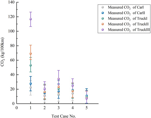
FIGURE 7. Test results of vehicles on circular curve sections with superelevation setting.

The prediction results show that the maximum relative errors of the carbon emission prediction results for passenger cars and trucks are 7.42% and 9.60%, respectively, which are less than 10%, indicating that the prediction level of the vehicle carbon emission model is higher in the circular curve section with superelevation setting.

(3) Transition curve section

The results of the passenger car and truck carbon emission tests on the transition curve test section are shown in Figure 8. R_-front、R_-back and L_c denote the radius of the circular curve before and after the transition curve section and the length of the transition curve section. For passenger cars and trucks, the maximum relative errors of the predicted and measured carbon emissions on the transition curve section are 7.40% and 8.09%, respectively, which are both less than 10%.

FIGURE 8

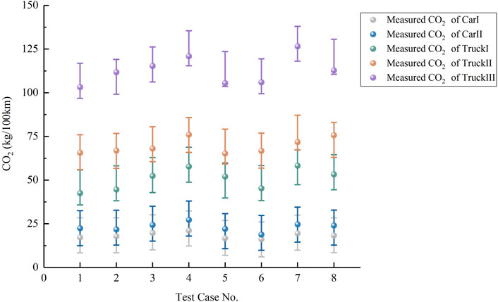
FIGURE 8. Test results of vehicles on transition curve section.

In addition to the assessment of the prediction accuracy of the model, the reliability of the model should also be examined. By analyzing the predicted and measured values of carbon emissions from vehicles on the horizontal curve sections, the consistency between the prediction results and the measured results is tested. The Adj-R² of the model is 0.915, indicating that the carbon emission model explains the measured data to a high degree. The asymptotic Sig of the chi-square test is 0.010, which is less than 0.05, indicating that the model explains the measured data to a high degree and is statistically significant.

The theoretical model shows that when a vehicle travels through a circular curve section at a constant speed, the lateral force coefficient does not change, and the curve driving resistance of the curve and its determined carbon emissions from the vehicle curve are constants. In the transition curve section where the curvature varies continuously, the vehicle curve carbon emission will change with it. Taking the horizontal curve measured at the automobile testing site as an example, the carbon emission profile of the vehicle traveling at a constant speed of 80 km/h is predicted and plotted as shown in Figure 9. It can visually characterize the carbon emission rules under different plane linear conditions. Among them, CO_2-Curve is used to reflect the influence of horizontal curve alignment on carbon emission.

FIGURE 9

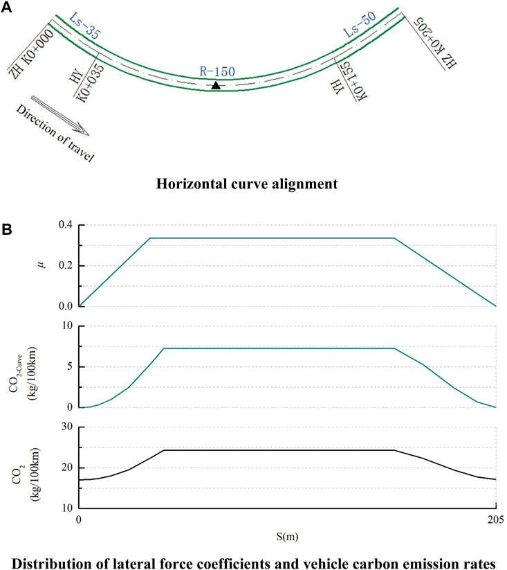
FIGURE 9. Vehicle carbon emission rates on horizontal curve sections. (A) geometric Design Specifications for Example Highway Horizontal Curves. (B) distribution of lateral force coefficients and vehicle carbon emission rates.

In Figure 9, the vehicle carbon emission rate of the gently curved section shows a horizontal segmental change. The vehicle carbon emission rate is a constant value in the circular curve section, and changes in the curve trend in the transition curve section. The longer the length of the transition curve is, the more gentle the change of vehicle carbon emission rate is.

3.3 Validation of vehicle carbon emission models for flat curve road sections under variable speed conditions

The test data under normal driving conditions on the circular curve section of the automobile test track are shown in Figure 10. The results show that for the test passenger cars and trucks, the maximum relative errors between the predicted and measured values of carbon emissions are 10.65% and 10.04% respectively, indicating that the model can reflect the carbon emissions under real driving conditions.

FIGURE 10

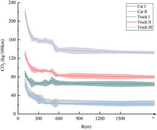
FIGURE 10. Normal driving test results of vehicles on circular curve section.

To test the statistical significance of the theoretical model in variable speed conditions, the model was subjected to residual analysis and likelihood ratio tests. The Adj-R² of the model is 0.925. The Durbin-Warson statistic was 1.592. The two-sided asymptotic Sig of the chi-square test is 0.010, which is less than 0.05. The results of these statistical tests indicate that the carbon emission model can explain the measured data well.

For planar lines, the transition curve can be regarded as a circular curve with gradually changing curvature. The carbon emission of the transition curve road section is equivalent to that of the circular road section with continuously changing curvature. It can be inferred that the accuracy of the carbon emission prediction of the transition curve road section and the circular road section is comparable. Due to time and site size constraints, and to avoid redundancy in the test program, this manuscript does not validate the modeling of vehicle carbon emissions on transition curve road sections with variable speeds.

To represent the impact of curve driving resistance and speed change on carbon emissions, the carbon emissions profile of a passenger car under normal driving conditions in the circular curve with a radius of 150 m and 400 m respectively are shown as an example, as shown in Figure 11. Among them, CO_2-Curve is used to visualize the effect of plane line shape on carbon emission, and CO_2-Velocity indicates the effect of speed change on carbon emission, whose value is determined by the air resistance, rolling resistance, and inertial resistance work done by the vehicle in the process of driving at variable speed in the flat straight road. The position of the midpoint of the curve is indicated by the symbol “▲”.

FIGURE 11

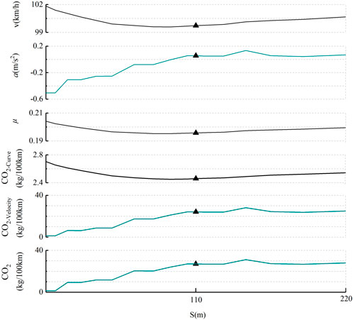
FIGURE 11. Carbon emissions under normal driving conditions on circular curve sections. (A) example of a circular curve with a radius of 150 meters. (B) the case of a circularl curve sections with a radius of 400 meters.

By analyzing the carbon emission curves in Figure 11, the following results can be obtained.

(1) In the first half of the circular curve with a radius of 150 m, the vehicle is traveling under braking and idling carbon emissions, which are illustrated by a dotted line in Figure 11A. The curve driving resistance is greater than the brake resistance and counteracts it, the vehicle has to overcome the remaining curve driving resistance, and the carbon emissions are at a low level, which is represented by a dotted line in Figure 11A. In the second half of the circular curve with a radius of 150 m, and in the whole length of the circular curve with a radius of 40 m, where the vehicle relies on engine-driven energy to drive, the trend of carbon emission and acceleration is same, and there is a high positive correlation between them.

(2) The smaller the radius, the more significant the degree of acceleration and deceleration, and the greater the magnitude of the change in carbon emissions.

(3) Under the above driving conditions, the speed fluctuations have a more significant effect on vehicle carbon emissions compared to the curve driving resistance.

(4) The trends of both vehicle turning carbon emissions and lateral force coefficients show a high degree of consistency.

Carbon emission tests were conducted on a circular curve section with consistent vehicle speeds to exclude the effect of speed variations on carbon emissions. The difference in carbon emissions when a vehicle is traveling at a constant speed on a curved and flat roadway, i.e., the incremental carbon emissions caused by the curve driving resistance. For trucks, this part of the carbon emission increment is caused by the curve driving resistance and suspension resistance. Based on the carbon emission model, the growth rate of carbon emission caused by vehicles turning at a constant speed can be predicted, see Figures 12, 13.

FIGURE 12

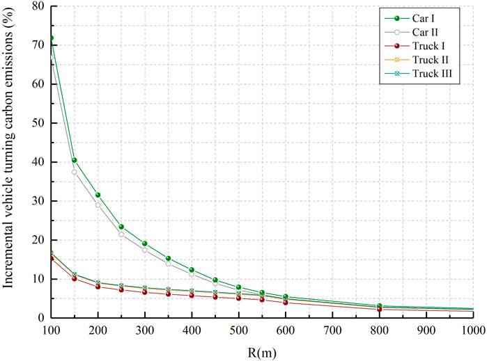
FIGURE 12. Incremental vehicle turning carbon emission.

FIGURE 13

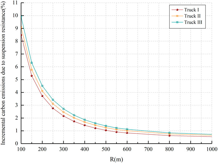
FIGURE 13. Incremental carbon emissions due to suspension resistance.

In Figures 12, 13, as the radius increases, the vehicle speed is gradually at a higher level, the lateral force coefficient gradually decreases, and the carbon emission decreases accordingly. Figure 12 shows that under the same road conditions, the growth rate of carbon emission caused by curve driving resistance is at different levels for passenger cars and trucks. According to the carbon emission theoretical model, the growth rate of a vehicle turning carbon emissions is determined by the geometric parameters of the curve (radius and superelevation) and the vehicle characteristics (including speed, load, tire characteristics, and tire number) and other factors. Passenger cars are commonly used for drivers’ daily access, and the loads are all small. Trucks are usually used for freight transportation, and the load capacity is larger. Heavy-duty vehicles focus on driving safety when crossing the curve, the speed is at a lower level. These factors affect the curve driving resistance differently, causing different growth rates of vehicle carbon emissions.

The difference between the carbon emissions of the test vehicle driving normally and at a constant speed in the circular curve section is the increment of carbon emissions caused by speed fluctuations. Its growth rate is shown in Figure 14.

FIGURE 14

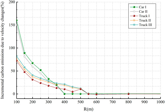
FIGURE 14. Incremental carbon emissions due to velocity changes.

In Figure 14, for passenger cars and heavy-duty vehicles, the radius of the circular curve is less than 400 m and 550 m, respectively, the growth rate of carbon emission caused by acceleration and deceleration behavior increases dramatically with the decrease of radius. In Figure 14, the growth rate of carbon emission caused by acceleration and deceleration is very small, not more than 1%, when the radius of the curve is larger than 400 m and 550 m, respectively.

Based on the analysis of the velocity data in Figure 3, the following results can be derived. When the radius of a circular curve is greater than or equal to 400 m and 550 m, respectively, passenger cars and trucks tend to drive through the curved road at a stable speed, and the effect of horizontal curves on carbon emissions is mainly reflected by the curve driving resistance. When the radius is less than 400 m and 550 m, respectively, passenger cars and trucks float more significantly, and carbon emissions are mainly affected by speed fluctuations, and carbon emissions increase sharply.

Unexpectedly, it was found that controlling the actual vehicle speed to be no greater than the operating speed at the midpoint of the curve and passing through the horizontal curve at a steady speed not only reduces the curve driving resistance, but also avoids additional carbon emissions caused by speed variations. The selection of the radius is closely related to the operating speed and superelevation. The design specification is often complied with in route design. Setting speed limits to adjust vehicle operating speeds when the route design parameters are constant is a practical guide to vehicle carbon emissions on constructed highways.

Based on the low-carbon theory, the maximum radius of the circular curve affecting the carbon emissions of passenger cars and trucks is 400 m and 550 m respectively, which can be used as a criterion to measure whether the design of horizontal curves is a basis for low-carbon and environmental protection. When the radius of the circular curve is smaller than this value, the carbon emission is mainly determined by the speed change, and it shows a sharp increase with the decrease of the radius. On the contrary, the incremental carbon emission of vehicles on curved road sections is mainly attributed to the effect of curve driving resistance.

4 Discussion

The Japan Road Association. (2004) conducted a field test on lateral force coefficients and fuel consumption, measured the growth rate of fuel consumption of small cars with different lateral force coefficients on the horizontal curved road section using the value of the lateral force coefficient as a control parameter. The speeds corresponding to different lateral force coefficients were not specified in the study. Considering that fuel consumption and carbon emissions are directly proportional, the growth rate of fuel consumption is equal to the growth rate of carbon emissions. The growth rate of carbon emissions due to lateral forces can be obtained by calculating the ratio of carbon emissions emitted by a vehicle traveling on a curved roadway to its emissions on a flat roadway. It can be viewed as the growth rate of carbon emissions due to curve-driving resistance. Based on the carbon emission model, the distribution range of the carbon emission growth profile can be predicted for different speeds and different lateral force coefficients. For the growth rate of carbon emissions, the measured results from the JRA against the model’s predictions are detailed in Figure 15.

FIGURE 15

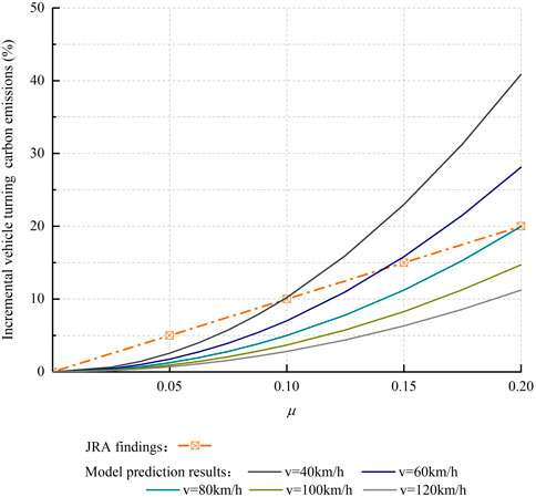
FIGURE 15. Growth rate of carbon emissions due to curve driving resistance to curves.

In Figure 15, the growth rate of carbon emissions is quadratically proportional to the lateral force coefficient under the same vehicle operating conditions. This proportionality has been described by the carbon emission prediction model. JRA used the measured statistical average speed to calculate the lateral force coefficient, weakening the relationship. The growth rate of carbon emission caused by the additional resistance of the curve shows a linear increasing trend. This supports the reliability of the carbon emission rules for vehicles on horizontal curve road sections proposed in this manuscript.

By comprehensively considering the direct and indirect effects of planar alignment on carbon emissions, this manuscript introduces the lateral force coefficient as the dependent variable and establishes a prediction model. In the model, the parameters that characterize the geometry of the horizontal curves that have an impact on carbon emissions are the radius of the circular curve, the superelevation, and the length of the transition curve. The larger the radius, the smaller the curve driving resistance and the lower the carbon emission. The setting of superelevation will reduce the lateral force coefficient, offset part of the centrifugal force, reduce the curve driving resistance, and thus reduce carbon emissions. Other research results can be summarized as follows.

1) The root cause of the increase in vehicle carbon emissions on horizontal curve sections is the curve driving resistance and speed fluctuations.

2) Under the free-flow driving condition of the actual highway, the maximum radius of the curve affecting the carbon emission of passenger cars and trucks is 400 m and 550 m, respectively. When the radius of the curve is smaller than the critical value, the carbon emission is mainly determined by the degree of acceleration and deceleration, and with the decrease of the radius, the carbon emission shows a sharp upward trend. On the other hand, the increase in carbon emission caused by speed fluctuations is very small, and the incremental carbon emissions is mainly attributed to the effect of the curve driving resistance.

3) In the process of low-carbon design of highways, by controlling the radius larger than the critical radius, the drastic increase of carbon emissions from curved traffic can be avoided.

4) In terms of low-carbon operation, the actual traveling speed of the vehicle is controlled to be no greater than the operating speed at the midpoint of the curve, and passing through the flat curve at a stable speed not only reduces the vehicle turning carbon emissions, but also avoids the additional carbon emissions caused by acceleration and deceleration.

5) The carbon emission rate of the uniform speed traveling on the horizontal curve sections shows a lateral segmental change. The carbon emission rate is a constant value in the circular curve section, and changes in the curve trend in the transition curve section. The longer the length of the transition curve, the more gentle the change of carbon emission rate.

6) When the vehicle relies on the driving energy from the engine to drive at variable speeds on horizontal curve sections, the carbon emission rate is the same as the change rules of acceleration.

The carbon emission model constructed in this manuscript is applies to the prediction of carbon emission under normal turning driving conditions, i.e., when the vehicle is in an accurate steering state with centrifugal acceleration of less than 0.4 g. In this case, the side deflection force is in the range of 0–2000 N and the side deflection angle is less than 3°(Mitschke and Wallentowitz, 2014). The model does not apply to the prediction of the vehicle in the state of understeer and oversteer.

5 Conclusion

In this study, a prediction model of vehicular carbon emissions on horizontal curve road sections is modeled, which can be realized to quantify the carbon emissions of traveling vehicles under different plane line conditions. The model characterizes the impact on carbon emissions in terms of the lateral force coefficient parameter regardless of the planar line shape. At the same time, a simplified test method is proposed to measure the carbon emissions of vehicles on different plane line conditions, i.e., by controlling the lateral force coefficient of the curved roadway as a dependent variable. Introducing the parameter of the transverse force coefficient can simplify the construction of the theoretical framework for the carbon emission of road vehicles under different planar geometries. At the same time, it can also reduce the implementation difficulty of the field test and shorten the test time and cost. The transverse force coefficient is determined by the radius of the circular curve, superelevation, and the length of the transition curve. Subsequent studies can be based on the model of this manuscript to further explore the degree of influence of each planar geometric linear indicator on carbon emission respectively, to put forward the suggested values of low carbon design for different planar linear indicators, and to realize the accurate and quantitative low carbon design of horizontal curve road sections.

Data availability statement

The original contributions presented in the study are included in the article/Supplementary Material, further inquiries can be directed to the corresponding authors.

Author contributions

YD: Conceptualization, Data curation, Formal Analysis, Funding acquisition, Methodology, Writing–original draft, Writing–review and editing. TL: Formal Analysis, Visualization, Writing–original draft. JX: Investigation, Supervision, Validation, Writing–review and editing.

Funding

The author(s) declare financial support was received for the research, authorship, and/or publication of this article. This research was funded by the Scientific Research Program of Shaanxi Provincial Education Department (Program No. 22JK0563), the Social Science Planning Fund of Xi’an City (23JX170), the Key Intelligent Database Research Project of Shaanxi Social Science Federation (2023ZD1100), the Natural Science Basic Research Plan in Shaanxi Province of China (2023-JC-QN-0261), the Qin Chuangyuan high-level innovation and entrepreneurship talent project (QCYRCXM-2022-242), the Social Science Foundation of Shaanxi Province of China (2023R361).

Conflict of interest

The authors declare that the research was conducted in the absence of any commercial or financial relationships that could be construed as a potential conflict of interest.

Publisher’s note

All claims expressed in this article are solely those of the authors and do not necessarily represent those of their affiliated organizations, or those of the publisher, the editors and the reviewers. Any product that may be evaluated in this article, or claim that may be made by its manufacturer, is not guaranteed or endorsed by the publisher.

References

Aashto, A. (2011). Policy on geometric design of highways and streets. 5th Edition. Washington, D. C. USA: American Association of State Highway and Transportation Officials, 231–240.

Google Scholar

Ataei, S. M., Aghayan, I., Pouresmaeili, M. A., Babaie, M., and Hadadi, F. (2021). The emission factor adjustments of the passenger cars in multi-story car parks under drive modes. Environ. Sci. Pollut. Res. 29, 5105–5123. doi:10.1007/s11356-021-15960-6

PubMed Abstract | CrossRef Full Text | Google Scholar

Bonneson, J. A. (2000). Superelevation distribution methods and transition designs NCHRP project 439. Washington, D. C: Transportation Research Board.

Google Scholar

Bonneson, J. A., and Pratt, M. P. (2009). Model for predicting speed along horizontal curves on two-lane highways. Transp. Res. Rec. 2092, 19–27. doi:10.3141/2092-03

CrossRef Full Text | Google Scholar

Cruz, P., Echaveguren, T., and González, P. (2017). Estimación del potencial de rollover de vehículos pesados usando principios de confiabilidad. Rev. Ing. Construccion 32 (1), 5–14. doi:10.4067/s0718-50732017000100001

CrossRef Full Text | Google Scholar

David, L., Ana, M. P., Alfredo, G., and García, A. (2018). Impact of horizontal geometric design of two-lane rural roads on vehicle CO₂ emissions. Transp. Res. Part D, Transp. Environ. 59, 46–57. doi:10.1016/j.trd.2017.12.020

CrossRef Full Text | Google Scholar

Ding, F., and Jin, H. (2018). On the optimal speed profile for eco-driving on curved roads. IEEE Trans. Intelligent Transp. Syst. 19, 4000–4010. doi:10.1109/tits.2018.2795602

CrossRef Full Text | Google Scholar

Dong, Y. P., Xu, J. L., and Gu, C. W. (2020). Modelling carbon emissions of diesel trucks on longitudinal slope sections in China. PlosOne 15 (6), e0234789. doi:10.1371/journal.pone.0234789

PubMed Abstract | CrossRef Full Text | Google Scholar

Dong, Y. P., Xu, J. L., Li, M. H., Jia, X., and Sun, C. (2019). Association of carbon emissions and circular curve in northwestern China. Sustainability 11 (4), 1156. doi:10.3390/su11041156

CrossRef Full Text | Google Scholar

Dong, Y. P., Xu, J. L., and Ni, J. (2023). Carbon emission model of vehicles driving at fluctuating speed on highway. Environ. Sci. Pollut. Res. 30 (7), 18064–18077. doi:10.1007/s11356-022-23064-y

CrossRef Full Text | Google Scholar

Faisal, A. (2005). Theoretical analysis for horizontal curves based on actual discomfort speed. J. Transp. Eng. 131 (11), 843–850. doi:10.1061/(asce)0733-947x(2005)131:11(843)

CrossRef Full Text | Google Scholar

Fitzpatrick, K., Elefteriadou, L., Harwood, D. W., Collins, J. M., McFadden, J., Anderson, I. B., et al. (2000). Speed prediction for two-lane rural highways, drivers. Available at: https://www.fhwa.dot.gov/publications/research/safety/ihsdm/99171.pdf (accessed on November 30, 2023).

Google Scholar

IPCC (Intergovernmental Panel on Climate Change) (2006). “Guidelines for national greenhouse gas inventories; prepared by the national greenhouse gas inventories program,” in IPCC-XLIX-9 – adoption and acceptance of 2019 refinement. Editors H. S. Egglestone, L. Buendia, K. Miwa, T. Ngara, and K. Tanabe (Tsukuba, Japan: IGES).

Google Scholar

Japan Road Association (2004). Explanation and application of road structure ordinance. Tokyo, Japan: Maruzen Publishing Co., Ltd.

Google Scholar

Ko, M. (2015). Incorporating vehicle emissions models into the geometric highway design process. Transp. Res. Rec. J. Transp. Res. Board 2503, 1–9. doi:10.3141/2503-01

CrossRef Full Text | Google Scholar

Lin, C. Y., Zhou, X. Y., Wu, D. Y., and Gong, B. W. (2019). Estimation of emissions at signalized intersections using an improved MOVES model with GPS data. Int. J. Environ. Res. Public Health 16, 3647. doi:10.3390/ijerph16193647

PubMed Abstract | CrossRef Full Text | Google Scholar

Mitschke, M., and Wallentowitz, H. (2014). Dynamik der Kraftfahrzeuge. 5nd Ed. Berlin: Springer Nature.

Google Scholar

Moradi, E., and Miranda-moreno, L. (2020). Vehicular fuel consumption estimation using real-world measures through cascaded machine learning modeling. Transp. Res. Part D 88, 102576. doi:10.1016/j.trd.2020.102576

CrossRef Full Text | Google Scholar

Pan, Y., Qiao, F., Tang, K., Chen, S., and Ukkusuri, S. V. (2020). Understanding and estimating the carbon dioxide emissions for urban buses at different road locations: a comparison between new-energy buses and conventional diesel buses. Sci. Total Environ. 703, 135533. doi:10.1016/j.scitotenv.2019.135533

PubMed Abstract | CrossRef Full Text | Google Scholar

Paolo, P. (2018). Influence of the general character of horizontal alignment on operating speed of two-lane rural roads. Transp. Res. Rec. 2075 (1), 16–23. doi:10.3141/2075-03

CrossRef Full Text | Google Scholar

Peng, J., Chu, L., and Fwa, T. F. (2020). Determination of safe vehicle speeds on wet horizontal pavement curves. Road Mater. Pavement Des. 22 (11), 2641–2653. doi:10.1080/14680629.2020.1772350

CrossRef Full Text | Google Scholar

Russo, F., Biancardo, S. A., and Busiello, M. (2016). Operating speed as A key factor in studying the driver behavior in a rural context. Transport 31 (2), 260–270. doi:10.3846/16484142.2016.1193054

CrossRef Full Text | Google Scholar

Sil, G., Nama, S., Asce, S. M., and Maurya, A. K. (2019). Modeling 85th percentile speed using spatially evaluated free-flow vehicles for consistency-based geometric design. J. Transp. Eng. 146 (2), 1–12. doi:10.1061/jtepbs.0000286

CrossRef Full Text | Google Scholar

Wang, X. M., Wang, X. S., Cai, B., and Liu, J. (2019). Combined alignment effects on deceleration and acceleration: a driving simulator study. Transp. Res. Part C Emerg. Technol. 104, 172–183. doi:10.1016/j.trc.2019.04.027

CrossRef Full Text | Google Scholar

Wen, H., and Eric, T. D. (2010). Models of acceleration and deceleration rates on A complex two-lane rural highway results from a night time driving experiment. Transp. Res. 12, 397–408. doi:10.1016/j.trf.2010.06.005

CrossRef Full Text | Google Scholar

Wong, J. Y. (2008). Theory of ground vehicles. 4th Edition. New York, USA: John Wiley& Sons, Ltd.

Google Scholar

Xu, J. L., Dong, Y. P., and Yan, M. H. (2020). A model for estimating passenger-car carbon emissions that accounts for uphill, downhill and flat roads. Sustainability 12 (5), 2028. doi:10.3390/su12052028

CrossRef Full Text | Google Scholar

Yin, Y., Wen, H., Sun, L., and Hou, W. (2020). Study on the influence of road geometry on vehicle lateral instability. J. Adv. Transp. 2020 (6), 1–15. doi:10.1155/2020/7943739

CrossRef Full Text | Google Scholar

You, S. S., and Jeong, S. K. (2002). Controller design and analysis for automatic steering of passenger cars. Mechatronics 12 (3), 427–446. doi:10.1016/s0957-4158(01)00005-8

CrossRef Full Text | Google Scholar

Zhang, L., Yu, L., Wang, Z., Zuo, L., and Song, J. (2016). All-wheel braking force allocation during a braking-in-turn maneuver for vehicles with the brake-by-wire system considering braking efficiency and stability. IEEE Trans. Veh. Technol. 65 (6), 4752–4767. doi:10.1109/TVT.2015.2473162

CrossRef Full Text | Google Scholar

Zhang, X., Xu, J., Li, M., Li, Q., and Yang, L. (2019). Modeling impacts of highway circular curve elements on heavy-duty diesel trucks’ CO₂ emissions. Int. J. Environ. Res. Public Health 16 (14), 2514. doi:10.3390/ijerph16142514

PubMed Abstract | CrossRef Full Text | Google Scholar