A novel machine learning ensemble forecasting model based on mixed frequency technology and multi-objective optimization for carbon trading price

Carbon trading prices are crucial for carbon emissions and transparent carbon market pricing. Previous studies mainly focused on data mining in the prediction direction to quantify carbon trading prices. Although the prospect of high-frequency data forecasting mechanisms is considerable, more mixed-frequency ensemble forecasting is needed for carbon trading prices. Therefore, this article designs a new type of ensemble prediction model to increase the scope of model research. The module is divided into three parts: data denoising, mixed frequency and machine learning, multi-objective optimization, and ensemble forecasting. Precisely, the data preprocessing technology enhanced by adopting a self-attention mechanism can better remove noise and extract effective features. Furthermore, mixed frequency technology is introduced into the machine learning model to achieve more comprehensive and efficient prediction, and a new evaluation criterion is proposed to measure the optimal submodel. Finally, the ensemble model based on deep learning strategy can effectively integrate the advantages of high-frequency and low-frequency data in complex datasets. At the same time, a new multi-objective optimization algorithm is proposed to optimize the parameters of the ensemble model, significantly improving the predictive ability of the integrated module. The results of four experiments and the Mean Absolute Percent Error index of the proposed model improved by 28.3526% compared to machine learning models, indicating that the ensemble model established can effectively address the time distribution characteristics and uncertainty issues predicted by carbon trading price models, which helps to mitigate climate change and develop a low-carbon economy.

1 Introduction

This part presents the relevant research background, a literature review, and the main contributions and innovations.

1.1 Research background

At present, climate change and reducing carbon dioxide emissions have become significant issues worldwide, and how to effectively reduce greenhouse gas emissions and curb global warming has become a common challenge for all countries (Wang Y. et al., 2022). The carbon market derives from the theory of environmental property rights and the theory of ecological modernization, which advocates market-based means to solve environmental problems (James and Menzies, 2022; Zhao et al., 2022; Emam and Tashkandy, 2023). It is an essential institutional innovation to promote the green and low-carbon transformation of economic development (Alhakami et al., 2022). The essence is to encourage companies to make decisions about emissions reductions by forming effective prices for trading carbon emissions through the mechanism of supply and demand (Taborianski and Pacca, 2022). The international carbon market has grown rapidly since the Kyoto Protocol came into force. In the academic community, carbon market research has attracted the attention of an increasing number of scholars (Han et al., 2019). Therefore, proposing an effective carbon trading price forecasting mechanism is crucial. The carbon trading price forecasting mechanism is the core issue in carbon Emissions (Wang F. et al., 2022; Yang et al., 2023).

1.2 Literature review

With vast amounts of methods to predict the stock market, researchers have devoted themselves to improving the accuracy of their models, including four types of methods: statistical technique, artificial intelligence technique, combined technique, and ensemble technique. In the literature review, we will examine the strengths and weaknesses of each of these approaches.

1.2.1 Statistical model

Statistical models have been widely used to predict stock markets. These models are based on historical data and use statistical techniques to identify patterns and correlations in the data (Li et al., 2022). For instance, Chai et al. employed an enhanced GARCH model for forecasting (Chai et al., 2023), and Guan et al. utilized an ARMA model to manipulate time series proficiently (Guan and Zhao, 2017). Although statistical models can still achieve good results, traditional statistical models need help capturing price changes’ complexity and nonlinear trends. Therefore, statistical models do not provide satisfactory results.

1.2.2 Artificial intelligence model

Artificial intelligence (AI) models are prevalent prediction models that have become increasingly popular in recent years. Gao et al. used multiple machine learning sub-models to predict crude oil price (Gao et al., 2022). Ruobin Gao et al. demonstrated the superiority of the ESN model in time series prediction (Gao et al., 2021). While Sun et al. used the LSTM model to predict carbon trading price, and the experiment showed that LSTM, as a deep learning model, is superior to general machine learning models (Sun and Huang, 2020). In addition, Borup et al. introduced a strategy of mixed frequency in machine learning to process high-frequency data more efficiently (Borup et al., 2023). Nevertheless, they should have capitalized on the strengths of each sub-model comprehensively. Besides, Machine learning models can become too complex during the training process, leading to overfitting of the training data and thus affecting the model’s generalization ability.

1.2.3 Combined model

To improve predictive ability, combined models combine multiple models to provide a more accurate prediction of stock prices (Xia et al., 2023). For example, a combined model may use a physical model to capture long-term trends, a traditional statistical model to capture short-term trends, and an AI model to identify patterns in the data. Wang et al. used the technique of calculating combined weights to combine the benefits of various machine learning models, enhancing the effectiveness of power load forecasting (Wang et al., 2021). In addition, Dong et al. introduced an LSTM model, which seamlessly integrated three sub-models, including a BPNN model (Dong et al., 2023). This combination leveraged the advantages of each sub-model and effectively captured the intricate characteristics of wave energy. However, there are challenges in determining the combined weight of each model.

1.2.4 Ensemble model

Ensemble prediction can provide a more comprehensive and reliable forecast of carbon trading prices by taking advantage of the strengths of different models and mitigating their weaknesses (Yang W. et al., 2022; Guo et al., 2022). Ensemble prediction is a powerful technique that can improve the accuracy of stock market prediction (Chullamonthon and Tangamchit, 2023). Wang et al. designed an ELM-based ensemble model optimized using the Sparrow Search Algorithm (SSA) for predicting carbon trading prices (Wang et al., 2022b). The model includes a VMD data preprocessing module, multi-objective optimization, and an ELM integration module. The prediction model Seçkin Karasu et al. proposed can handle the chaos and non-linear dynamics of WTI and Brent COTS. In recent years, multi-objective optimization techniques have been widely applied to optimize the parameters of ensemble models to improve experimental results. Yang et al. used multi-objective Ant Lion Optimizer (MOALO) to optimize their prediction results (Yang H. et al., 2022). Meanwhile, Fallahi et al. also used the Multi-Objective Grey Wolf Optimizer (MOGWO) to improve the accuracy of carbon emission reduction prediction results (Fallahi et al., 2023). In addition to multi-objective optimization ensemble models, Liang Dua et al. successfully synthesized ten candidate models using a Bayesian dynamic ensemble method, which has higher adaptability and better generalization performance (Du et al., 2022). Ensemble models have also successfully addressed the non-linear features of time series prediction. For example, the digital currency prediction hybrid model proposed by Aytaç Altan et al. can capture the non-linear characteristics of digital currency time series (Altan et al., 2019). The prediction model proposed by Seçkin Karasu et al. can also capture the non-linear characteristics of crude oil time series, with better prediction performance in terms of accuracy and volatility than existing prediction models (Karasu et al., 2020; Karasu and Altan, 2022). Therefore, ensemble models can better integrate the strengths of different models to improve the accuracy of carbon trading price prediction while also playing an important role in capturing non-linear features.

Although the current carbon trading price forecasting system is developing rapidly, some issues still need to be considered in future development. Early research mainly focused on common frequency research (Niu et al., 2022), with less use of mixed frequency techniques. To better handle the impact of high-frequency data on complex datasets with low-frequency data, Lahiri et al. improved their predictive ability by using mixed frequency techniques and a single model to predict New York State tax revenue (Lahiri and Yang, 2022). Chang et al. used a single mixed frequency model for carbon emission prediction (Chang et al., 2023). Jiang et al. used a single MIDAS model to explore the relationship between carbon emissions and economic growth, fully leveraging the advantages of mixed frequency techniques (Jiang and Yu, 2023). In the era of big data, researchers can obtain time series data at different frequencies, where high-frequency information has the advantages of timeliness and stability relative to low-frequency information. In carbon trading price prediction, high-frequency data usually has a higher update frequency and can reflect the dynamic changes in market prices more timely. High-frequency data is essential for decision-makers who need to respond quickly because high-frequency data can provide more timely predictions and decision support. In addition, high-frequency data is relatively stable as it better captures the microstructure and behavior of the market, which means that high-frequency data can provide more stable prediction results, reducing the volatility and uncertainty of predictions. Therefore, mixed frequency prediction has yet to be considered in the current carbon trading price prediction field, or the impact of ensemble models and mixed frequency techniques needs to be considered.

Therefore, Some issues exist in the current carbon trading price forecasting field: Lack of technical updates in data mining, such as disregard for mixed-frequency prediction and indifference towards ensemble models utilizing mixed-frequency techniques. Specifically, most carbon trading price prediction studies use time series analysis, machine learning, and other methods to mine historical price data to predict future price trends. However, this approach often needs to pay more attention to the interactions and impacts between different frequency data. Therefore, when building an ensemble forecasting model, it is necessary to consider the influence of both high-frequency and low-frequency data to predict carbon trading prices more accurately. In addition, the current mainstream data preprocessing method, VMD, has an issue of uncertain decomposition mode, which reduces the predictive power of the ensemble model. If the number of modes decomposed by VMD is too small, important price fluctuation features may be missed. These unconsidered features may significantly impact the prediction results, leading to a decrease in prediction accuracy. On the other hand, if the number of modes decomposed by VMD is too large, mode overlap may occur. Mode overlap means that some modes may overlap or interact, making the prediction model complex and challenging to interpret and reducing the model’s predictive power and robustness. In conclusion, there are the following issues:

(1) Neglecting mixed-frequency prediction and having an indifferent attitude towards integrated models utilizing mixed-frequency techniques, i.e., giving less consideration to the temporal distribution characteristics of carbon trading prices.

(2) The current mainstream data preprocessing method VMD has the problem of uncertain decomposition patterns. Additionally, both the sub-models and ensemble models suffer from parameter randomness, leading to the issue of parameter uncertainty in carbon trading price prediction.

In order to address these issues, this research aims to consider and resolve the temporal distribution characteristics and uncertainties of carbon trading prices better. Specifically, this study develops a novel ensemble forecasting method comprised of three modules to predict carbon trading prices. Firstly, the data preprocessing module employs effective methods to address the prediction uncertainties in carbon trading prices. As high-frequency data may contain more noise and fluctuations, the VMD decomposition technique has an advantage over EMD and EWT in decomposing complex and nonlinear data because it can better overcome the mode mixing problem of EMD and EWT by using a constrained variational problem, resulting in more accurate decomposition results (Lian et al., 2018; Huang et al., 2021). However, the original VMD technique may need more accurate forecasting due to randomly chosen decomposition mode numbers. Recently, self-attention mechanisms have been shown to effectively mitigate this issue by comparing the similarity between the vectors of the ground truth and predicted values (Chen et al., 2023), thereby determining the number of modal decompositions. Therefore, this study proposes a new data preprocessing method called SA-VMD to improve the drawback of uncertain mode decomposition numbers in VMD. Additionally, the current research framework mainly focuses on the influence of traditional energy sources on carbon trading prices, as mentioned by Song et al. regarding the significant impact of natural gas, fuel oil, and crude oil prices on carbon trading prices (Song et al., 2022). However, the research overlooks clean energy sources (Hao and Tian, 2020). Wang et al. mention the correlation between ethanol and carbon trading price predictions (Wang et al., 2023). Therefore, this study incorporates ethanol data and considers four multivariate factors: natural gas, fuel oil, crude oil, and ethanol. Secondly, in the mixed-frequency and machine learning module, this study utilizes the Mixed Data Sampling (MIDAS) model to transform the high-frequency data of the four factors into low-frequency data for predicting carbon trading prices. Simultaneously, three low-frequency machine learning models are employed for comparative experiments in mixed-frequency prediction, which better accounts for the temporal distribution characteristics in carbon trading price prediction. Furthermore, a newly proposed evaluation criterion can better determine the models’ lag order and other parameter information, thus avoiding errors caused by parameter uncertainties. Finally, LSTM is chosen as the deep learning tool in the ensemble module due to its powerful learning capabilities. The ensemble model can fully leverage the advantages of each sub-model and capture the nonlinear features of carbon trading prices. To address the issue of parameter uncertainties in carbon trading price prediction, this study optimizes the parameters of the LSTM model based on Multi-Objective Whale Optimization (MOWSO), reducing the uncertainty and improving the accuracy and stability of price predictions. This study constructs a new framework for carbon price prediction by integrating the effects of three machine learning models based on four multivariate factors and four mixed-frequency models. This framework fully considers the temporal distribution characteristics of carbon trading price prediction by harnessing the advantages of integrating high-frequency and low-frequency data using LSTM. It aims to address current research gaps, fill in the research void, and ultimately provide a new framework for carbon price prediction.

1.2.5 Contributions and innovations

The data preprocessing modules proposed, including the mixed frequency and machine learning module and ensemble forecasting module, were used to develop a new deep learning model ensemble system. In summary, the proposed new ensemble model can effectively improve the forecasting performance of carbon trading prices and lay the foundation for better use of mixed frequency technology prediction methods.

The contributions and innovations can be summarized as follows:

(1) Efficient data preprocessing methods. Data preprocessing technology can improve data quality and help enhance subsequent prediction processes’ accuracy and performance. Previous research employed VMD data preprocessing algorithms that contained an uncertainty in the number of modes to be decomposed, leading to decreased prediction accuracy. This paper uses self-attention-variational mode decomposition (SA-VMD) to obtain better prediction results than VMD techniques to eliminate this uncertainty in the number of modes to be decomposed in VMD. The experiment shows that after data preprocessing, the sub-model improves prediction performance and stability compared to the corresponding sub-model.

(2) Capable mixed frequency technology. To better consider the impact of different periodic factors on the prediction experiment, this article considers the effect of mixed frequencies on carbon price prediction. The introduction of mixing technology not only compensates for the previous studies that did not consider the impact of different cycle factors on the experiment but also lays a solid foundation for proposing novel ensemble prediction modules. Experiments have shown that excellent sub-models can be created using novel mixed frequency and common frequency techniques in the proposed modeling module.

(3) Excellent multi-objective optimizer and ensemble model. In the current carbon trading price forecasting model, only some studies simultaneously consider the effects of high-frequency and low-frequency data. To better integrate the strengths of common frequency, mixed frequency, and deep learning ensemble strategies, this article considers using the LSTM model to integrate the mixed frequency and the common frequency models. At the same time, a new recently proposed multiobjective algorithm is introduced to optimize the three parameters of the ensemble model and predict the performance based on the carbon trading price. The successful experiment proves that the new ensemble system effectively improves the accuracy and stability of predicting carbon trading prices.

2 Framework of the novel ensemble forecasting system for the carbon trading price

The ensemble forecasting model for carbon emissions trading developed in this paper is shown in Figure 1, and the framework is listed in detail below:

FIGURE 1

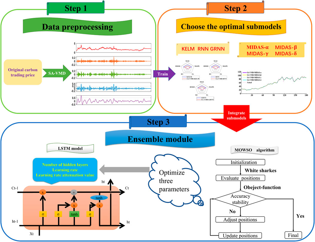
FIGURE 1. Flowchart of the forecasting model.

Stage 1: Since data preprocessing makes the data reliable and interpretable and enables effective investigation, SA-VMD is used to process the original data in this work. SA-VMD has high robustness to sampling and noise and can effectively avoid modal aliasing. Through the data preprocessing method, this paper effectively removes the noise and preserves the main features of the original data.

Stage 2: Measure the machine learning and mixed frequency models using new evaluation criteria to obtain the optimal partial model in each case. The evaluation criteria were successfully used to obtain the optimal sub-models of four mixed frequencies and three machine learning models to take the best advantage of mixed frequencies, which provide a basis for the ensemble prediction of carbon trading prices.

Stage 3: Considering the powerful learning ability of machine learning, this paper selects the LSTM model in the machine learning model and uses an innovative multi-objective algorithm to find the optimal solution for the hidden LSTM layer, learning rate, and learning rate attenuation value to obtain the final ensemble model.

3 Novel ensemble predicting model modules

The novel ensemble prediction model consists of the data preparation module, the mixed frequency module, the machine learning module, and the ensemble modeling module.

3.1 Data preparation module

3.1.1 Variational mode decomposition

VMD is a powerful signal processing technique that gained widespread acceptance in the last few years (Dragomiretskiy and Zosso, 2013). The basic idea behind VMD is to decompose a given signal into a series of elementary modes or components, each with frequency and amplitude characteristics. These components are combined to reconstruct the original signal, each component making up a specific part of the overall signal.

The mathematical basis of VMD can be complex. However, at its core, it finds a set of optimal functions (intrinsic mode functions) that can effectively represent the input signal. These mode functions are determined by solving an optimization problem that minimizes the difference between the signal and its decomposition.

Suppose $u_p=\left\{u_1,u_2,\dots ,u_P\right\}$ is the Kth Intrinsic Mode Functions obtained from decomposition, ${\omega }_p=\left\{{\omega }_1,{\omega }_2,\dots ,{\omega }_P\right\}$ means the center frequency of each component. δ_t, f(t), and * represent impulse function, original signal, and convolutional operator, respectively. Optimization problem mentioned above, which is also a variational question, lists as follows:

$\left\{\begin{array}{c}\hfill \underset{u_p,{\omega }_p}{\min }\left\{\sum _{p=1}^P\Vert {\partial }_t\left[\left(\delta \left(t\right)+\frac{j}{\pi t}\right)\cdot u_p\left(t\right)\right]e^{-j{\omega }_{m}t}{\Vert }_2^2\right\}\hfill \\ \hfill \text{s}.t.\sum _{p=1}^P{u}_p=f\left(t\right)\hfill \end{array}\right.(1)$

To solve this problem, the above problem can be transformed into a variational problem without constraint by an augmented Lagrangian function by introducing the penalty factor α and the Lagrange multiplier γ.

$\begin{array}{ll}\hfill L\left(u_p,w_p,\lambda \right)& =\alpha \sum _{p=1}^P{‖{\partial }_t\left[\left(\delta \left(t\right)+\frac{j}{\pi t}\right)\cdot u_p\left(t\right)\right]e^{-j{w}_{p}t}‖}_2^2\hfill \\ \hfill & +{‖f\left(t\right)-\sum _{p=1}^p{u}_p\left(t\right)‖}_2^2+⟨\lambda \left(t\right),f\left(t\right)-\sum _{p=1}^P{u}_p\left(t\right)⟩\hfill \end{array}(2)$

The problem can be solved using the alternating direction multiplier method (ADMM). The idea is to fix the other two variables and update one of them as follows:

$\begin{array}{cc}\hfill & u_p^{n+1}=\underset{u_p}{\mathrm{arg\; min}}L\left(\left\{u_{i<p}^{n+1}\right\},\left\{{\omega }_p^n\right\},{\lambda }^n\right)\hfill \\ \hfill & {\omega }_p^{n+1}=\underset{{\omega }_k}{\mathrm{arg\; min}}L\left(\left\{u_p^n\right\},\left\{{\omega }_{i<p}^{n+1}\right\},{\lambda }^n\right)\hfill \\ \hfill & {\lambda }^{n+1}={\lambda }^n+\rho \left(f\left(t\right)-\sum _p{u}_p^{n+1}\left(t\right)\right)\hfill \end{array}(3)$

Taking the derivative of the above equation in the frequency domain, we can conclude that:

${\widehat{u}}_p^{n+1}=\frac{\widehat{f}\left(\omega \right)-\sum _{i\ne p}{\widehat{u}}_i\left(\omega \right)+\frac{\widehat{\lambda }\left(\omega \right)}{2}}{1+2\alpha {\left(\omega -{\omega }_p\right)}^2}(4)$

Similarly, it can be concluded that:

${\widehat{\omega }}_p^{n+1}=\frac{{\int }_0^{\infty }\omega \left|{\widehat{u}}_p\left(\omega \right)\right|d\omega }{{\int }_0^{\infty }\left|{\widehat{u}}_p\left(\omega \right)\right|d\omega }(5)$

${\widehat{\lambda }}^{n+1}\left(w\right)={\widehat{\lambda }}^n\left(w\right)+\tau \left[\widehat{f}\left(w\right)-\sum _m{\widehat{u}}_p^{n+1}\left(w\right)\right](6)$

3.1.2 Self attention-variational mode decomposition

The self-attention (SA) mechanism is an effective method for obtaining information that has emerged in machine learning in recent years. Yuan et al. improved the EMD algorithm based on the SA mechanism (Yuan and Yang, 2023). Usually, VMD decomposition achieves the effect of data preprocessing by randomly setting the number of decomposition modes and removing the high-frequency part of the data. However, this method may have the problem of excessive error (Gao et al., 2023). In order to avoid randomly selecting the number of decomposed modes as much as possible, this article will improve the VMD noise reduction method using the SA method.

In traditional sequence models, such as recurrent neural networks (RNNs), the representation of each position can only be obtained through sequential processing to get contextual information. The self-attention mechanism allows each part to focus directly on other elements in the input sequence to receive more comprehensive contextual details. At the same time, the self-attention mechanism obtains weights by calculating the correlation between each position and other positions. Then, it applies these weights to the weighted sum of all parts in the input sequence. In this way, the representation of each location can contain information from other places.

The advantage of the self-attention mechanism is that it can calculate the correlation between various positions in parallel without relying on sequential processing like traditional recurrent neural networks. To better utilize the advantages of the self-attention mechanism to improve VMD, it is considered to determine the most suitable number of patterns by calculating the cosine angle value corresponding to the original data after data preprocessing. The smaller the absolute value of the included angle, the higher the correlation between the two. The relationship between the original data and the target can be successfully measured by calculating cosine similarity to select an appropriate number of decomposition modes.

$sim\left(\widehat{Y_m},Y_m\right)=\left|\frac{{\widehat{Y_m}}^T\cdot Y_m}{\Vert \widehat{Y_m}\Vert *\Vert Y_m\Vert }\right|(7)$

Where $\widehat{Y_m}$ and Y_m represent the component obtained after VMD decomposition and the component of original data, respectively, while m = 1, 2, … , M denotes the number of decomposition modes.

3.2 Mixed frequency and machine learning modules

To better leverage the role of data preprocessing, it is crucial to propose effective artificial intelligence models. Mixed frequency and machine learning modules are introduced to increase the impact of different cycles on the results.

3.2.1 Mixed frequency model

MIDAS (Mixed Data Sampling) regression is a method for predicting time series data that combines high-frequency and low-frequency data (Ghysels and Valkanov, 2004). This technique has been applied in various fields, including finance, economics, and environmental studies.

The basic idea of MIDAS regression is to use high-frequency data as independent variables and low-frequency data as dependent variables (Xu et al., 2021; Wichitaksorn, 2022). The approach involves fitting a regression model in which the independent variables are lagged high-frequency data, and the dependent variable is low-frequency data. The mathematical formula for the MIDAS regression model is as follows:

$Y_t={\beta }_0+{\beta }_{1}B\left(L^{1/m};\theta \right)X_t^{\left(m\right)}+{\epsilon }_t(8)$

where Y_t, X_t represent the low-frequency data and the high-frequency data, respectively, at time v. m is the value obtained by dividing the high frequency by the low frequency and will be 7 in this article. ɛ_t is the residual term. L^k/m lags the value of X_t backward by k, and their specific mathematical expressions are listed as follows:

$\begin{array}{cc}\hfill L^{k/m}{X}_t^m& =X_{t-k/m}^{\left(m\right)}\hfill \\ \hfill B\left(L^{1/m};\theta \right)& =\sum _{k=0}^K\omega \left(k;\theta \right)L^{k/m}\hfill \end{array}(9)$

where K denotes the maximum delay order of Y_v, and $\omega \left(k;\theta \right)$ is a polynomial function that includes some common functions such as the beta polynomial, etc.

A variant of the MIDAS model is the autoregressive MIDAS (AR-MIDAS) model, which extends the basic MIDAS model with autoregressive terms for the dependent variable. This allows modeling of time-varying coefficients and dynamics in the relationship between variables. The AR-MIDAS model is represented as follows:

$Y_t={\beta }_0+\sum _{l=1}^L{\eta }_l{Y}_{t-l}+{\beta }_{1}B\left(L^{1/m};\theta \right)X_{t/m}^{\left(m\right)}+{\epsilon }_v(10)$

Similar to the above lag of the low-frequency variables, introducing the step size h to lag the high-frequency variables also improves the result of the prediction.

$Y_t={\beta }_0+\sum _{l=1}^L{\eta }_l{Y}_{t-l}+{\beta }_{1}B\left(L^{1/m};\theta \right)X_{t-h/m}^{\left(m\right)}+{\epsilon }_v(11)$

For the convenience of abbreviation, the following notation will be used later. The impact of gas on carbon emissions is captured as MIDAS-α, while the impact of fuel oil, crude oil, and ethanol on carbon emissions are referred to as MIDAS-β, MIDAS-γ, and MIDAS-δ, respectively.

3.2.2 Machine learning model

Artificial neural network (ANN) prediction is a type of machine learning that uses algorithms to model and predict complex relationships between inputs and outputs. The ANN consists of multiple layers of interconnected nodes or artificial neurons, which make predictions based on patterns in the data.

3.2.2.1 Kernel extreme learning machine

The Extreme Learning Machine (ELM) is a powerful model that has gained popularity in recent years due to its ability to make fast and accurate predictions (Huang et al., 2006). The ELM model is a type of feedforward neural network that can be trained quickly and efficiently, making it ideal for large data sets.

The connecting weight β is between the hidden layer and the output layer. The output of hidden layer nodes and output are denoted as H, T respectively. ELM model can be expressed as:

$H\beta =T^{\prime }(12)$

While the minimum of the loss function can get the value of β.

$\beta ={\left(H^{T}H\right)}^{-1}{H}^{T}T(13)$

The Kernel Extreme Learning Machine (KELM) is an extended version of the ELM model that includes kernel features to improve accuracy and performance. Like the ELM model, the KELM is a feedforward neural network that uses a random weight initialization process to speed up training, but instead of a single hidden layer with linear activation functions, it incorporates kernel functions to handle non-linear relationships between input and hidden layers (Huang et al., 2011). This allows the model to capture more complex relationships in the data, resulting in higher accuracy and better performance (He et al., 2020).

$\beta =H^T{\left(H^{T}H+\frac{I}{C}\right)}^{-1}T(14)$

3.2.2.2 Recurrent neural network

Recurrent neural network (RNN) are a powerful type of artificial neural network that are particularly well suited for predicting sequential data (Medsker and Jain, 2001). RNN consist of a series of interconnected nodes or “cells” that are capable of both receiving and transmitting information (Park et al., 2020).

One of the main advantages of RNN is their ability to learn long-term dependencies between inputs. In this way, the network can detect patterns in the input data that occur over long periods of time, such as seasonal trends or periodic fluctuations (Son et al., 2019).

The RNN has only two inputs: x_t and h_t−1. These two inputs are the sample input at the current time and the hidden layer state input at the previous time. We fix h_t−1, so we only change x_t. Two outputs in the RNN are O_t and h_t. These two outputs are the output of the current time step and the output of the hidden layer of the current time step. The current transition of the hidden layer is used as input for the calculation of the next time step.

Assume σ, W, c are activation function, weight and bias, respectively. The calculation formulas from input to output O_t and h_t are listed as follows:

$\begin{array}{cc}\hfill h_t& =\sigma \left(U*x_t+V*h_{t-1}+b\right)\hfill \\ \hfill O_t& =W*h_t+c\hfill \end{array}(15)$

3.2.2.3 General regression neural network

GRNN is a network-based model which can be used for tasks such as classification, regression, and clustering (Specht et al., 1991). The full name of GRNN is General Regression Neural Network and was proposed by American scientist Donald F. Specht.

The advantage of GRNN is that it does not require too much parameter adjustment and training time, and it works well even with small data sets. In addition, GRNN is also very resistant to noise and high interpretability, which makes it widely applicable in practise.

The theoretical basis of GRNN is nonlinear regression analysis, in which the analysis of the nonindependent variable Y with respect to the independent variable u actually computes v with the maximum probability value. Let the observed value of u be known to be u, then let the regression of v be with respect to X. Where X_i, Y_i are the sample observations of the random variables u, v. σ is the width coefficient of the Gaussian function. Computing a net output $\widehat{Y}(X)$ as:

$\widehat{Y}\left(X\right)=\frac{\sum _{i=1}^n{Y}_i{e}^{-\frac{{\left(X-X_i\right)}^T\left(X-X_i\right)}{2{\sigma }^2}}}{\sum _{i=1}^n{e}^{-\frac{{\left(X-X_i\right)}^T\left(X-X_i\right)}{2{\sigma }^2}}}(16)$

3.2.2.4 Long short-term memory network

LSTM is a variant of RNN to solve the long-term memory problem (Hochreiter and Schmidhuber, 1997).

LSTM has certain advantage in sequence modeling and has a long-term memory function which leads to implementation easily (Gallardo-Antolín and Montero, 2021). Meanwhile, LSTM solves the problem of gradient vanishing and gradient explosion during long sequence training (Hao et al., 2022). As a deep learning machine learning model, LSTM has the advantage of significantly improving prediction performance and has been increasingly noticed and used by scholars. Meanwhile, LSTM is a network commonly used for sequence model prediction, widely used in fields such as time series analysis (Akhtar and Feng, 2022). LSTM has strong anti-noise performance. When processing sequence data in practical applications, there are often situations where noise and outliers exist in the data (Alsulami et al., 2022).

The gate structure of LSTM (3 in total) is listed as follows:

◦ Forget Gate: based on the current input and the previous state of the hidden layer, the sigmoid activation function is used to determine which information to forget.

$f_t=\sigma \left(W_f\cdot \left[h_{t-1},i_t\right]+b_f\right)(17)$

◦ Input Gate: after some information is forgotten, it is necessary to add some useful information based on the last state, and at this point an input gate is used to determine what information is newly added.

$\begin{array}{cc}\hfill m_t& =\sigma \left(W_m\cdot \left[h_{t-1},i_t\right]+b_m\right)\hfill \\ \hfill {\tilde{C}}_t& =\tanh \left(W_C\cdot \left[h_{t-1},i_t\right]+b_C\right)\hfill \\ \hfill C_t& =f_t*C_{t-1}+m_t*{\tilde{C}}_t\hfill \end{array}(18)$

◦ Output Gate: the output gate determines the output at the current time based on the input at the current time, the state of the hidden layer at the previous time, and the last state.

$\begin{array}{cc}\hfill o_t& =\sigma \left(W_o\left[h_{t-1},i_t\right]+b_o\right)\hfill \\ \hfill h_t& =o_t*\tanh \left(C_t\right)\hfill \end{array}(19)$

Where i_t, f_t, C_t, o_t and ${\tilde{C}}_t$ are the input value, forget gate, input gate, and input gate, the unit state, respectively. h_t−1 is output at the previous time step. σ is the sigmoid function, W and b are weights and biases parameters.

In conclusion, LSTM networks offer several advantages and unique features that make them powerful tools for integrating models with commen frequency and mixed frequency. Although LSTM is a widely used deep learning model, the number of hidden layers and the value of the learning rate are uncertain, which leads to its instability. The multiobjective algorithm is used to find the optimal number of hidden layers, learning rate, and learning rate attenuation value.

3.3 Ensemble modeling module

To enhance the results of prediction, an ensemble predictor based on multi-objective algorithms is developed as an ensemble prediction component in this paper.

3.3.1 Multi-objective optimization techniques

White Shark Optimizer (WSO) is a new algorithm proposed by Malik Braik, Abdelaziz Hammuri et al., inspired by the behavior of the great white shark during hunting (Braik et al., 2022). Improved multi-objective WSO algorithm (MOWSO) was proposed to solve multi-objective optimization problems (Xing et al., 2023). The details are described below:

WSO needs to be initialized before the iteration starts, and the initial solution is represented by the following equation:

$\omega =\left[\begin{array}{c}\hfill W_{11}{W}_{12}\dots W_{1n}\hfill \\ \hfill W_{21}{W}_{21}\dots W_{2n}\hfill \\ \hfill ⋮⋮⋮\hfill \\ \hfill W_{d1}{W}_{d2}\dots W_{dn}\hfill \end{array}\right](20)$

The dimensional of the space is n, the population of d great white sharks (i.e., the population size) and the location of each great white shark can be represented as a d-dimensional matrix to represent the proposed solutions to a problem.

$W_{ji}=L_i+r\times \left(L_i-U_i\right)(21)$

W_ji is the initial vector of the jth white shark in the ith dimension. U_i and L_i represent the lower and upper bounds of the space in the ith dimension, respectively. r is a random number created in the interval [0, 1]. And k and K stand for the current and maximum number of iterations.

The speed to the prey:

$V_{k+1}^j=\mu \left[V_k^j+P_1\left(W_{\text{gb\hspace{0.17em}}}-W_k^j\right)\times C_1+P_2\left(W_{\text{b\hspace{0.17em}}}-W_k^j\right)\times C_2\right](22)$

Where j = 1, 2, … , d is the great white shark of the n large population, $V_{(k+1)}^j$ represents the new velocity vector at step (k + 1), $V_k^j$ defines the current velocity vector at step k, W_gb represents the global optimal position vector achieved by each great white shark in the kth iteration so far, $W_k^j$ is the current position vector of the first great white shark in step k, W_b is the best known position vector of the population, and C₁, C₂ are two random numbers generated uniformly in the range of [0, 1]. μ refers to the constriction factor proposed in WSO. P₁ and P₂ represent the forces of the white sharks that control the effect of W_gb and W_b on $V_k^j$.

Approaching the best prey:

$W_{k+1}^j=\left\{\begin{array}{cc}{W}_k^j\times \mathrm{\Lambda }\oplus +\left(u\times t_1\right)+\left(u\times t_2\right)\hfill & \text{\hspace{0.17em}rand\hspace{0.17em}}<mv\hfill \\ W_k^i+\left(W_k^j/f\right)\hfill & \text{\hspace{0.17em}rand\hspace{0.17em}}\ge mv\hfill \end{array}\right.(23)$

Among them, $t_1=sgn(W_k^j-u)>0$ and $t_2=sgn(W_k^j-l)<0$ represent one-dimensional binary vectors determined by the formula, f denotes the frequency parameters mv of the waves, Λ is a negation operator, ⊕ is a bit-wise xor operation, which are supposed to express the auditory and olfactory intensity of the great white sharks, increasing as an iterative function. rand defines a random number created in the range from 0 to 1, and u denotes the lower and upper limits of the search space. A smaller value mv leads to a local search, while a larger value mv leads to a global search, where mv is represented by the following equation:

$mv=\frac{1}{\left(a_0+e^{\frac{K/2-K}{a_1}}\right)}(24)$

Where a₀ and a₁ are two positive constants employed to manage exploration and exploitation behaviors.

Optimal positional motion (convergence):

${W_{k+1}^j}^{\prime }=W_{\text{gb}}+p_1{D}_w\mathrm{s}\mathrm{g}\mathrm{n}\left(p_2-0.5\right)p_3<S(25)$

${W_{k+1}^j}^{\prime }$ is the updated location of the jth great white shark relative to its prey location, sgn (p₂ − 0.5) gives 1 or −1 for the change in search direction. p1, p2 and p3 are random numbers in the range [0, 1], D_ω is the distance between the prey and the great white shark, and S is the odor and sight intensity of the proposed parameter great white shark when following other great white sharks near the best prey.

3.3.2 Ensemble forecasting module

In this section, the new ensemble strategy integrates the submodels to acquire the ultimate carbon trading price forecasting results. Considering the advantages of Deep Learning in machine learning and price forecasting (Lin et al., 2022), this paper attempts to develop a novel ensemble predicting model based on the LSTM model as an ensemble forecasting model. Although LSTM is a widely used deep learning model, the number of hidden layers and the learning rate’s value are uncertain, leading to its instability. To overcome this problem, this paper considers introducing an advanced MOWSO algorithm to solve this problem. The multiobjective algorithm finds the optimal number of hidden layers, learning rate, and learning rate attenuation value. Among them, accuracy and stability are represented by f₁ and f₂ respectively, as shown below:

$\min \left\{\begin{array}{c}{f}_1=\frac{1}{L}\sum _{t=1}^L{\left(|{\widehat{A}}_l-A_l|\right)}^2\hfill \\ f_2=\mathrm{S}\mathrm{t}\mathrm{d}\left(|{\widehat{A}}_l-A_l|\right)\hfill \end{array}\right.(26)$

Where A_l and ${\widehat{A}}_l$ represent the actual and predicted values, respectively. t = 1, 2, … , L, L is the test sample size.

By combining the advantages of LSTM and MOWSO, a MOWSO-LSTM model is built to obtain the optimal parameter solution and objective function value. Finally, based on the MOWSO-LSTM model, a novel ensemble forecasting model is proposed, which provides an optimal prediction of carbon trading prices by integrating the advantages of each sub-model. Table 1 presents the parameter values employed in this study for the MOWSO optimization algorithm and the LSTM deep learning model.

TABLE 1

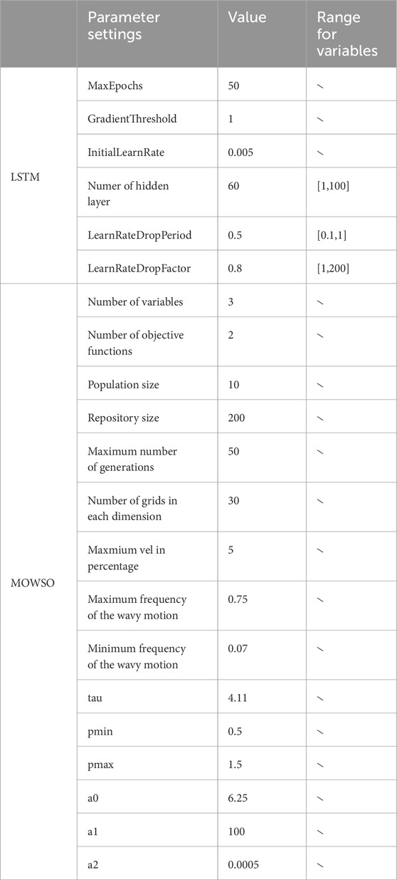
TABLE 1. Parameter values utilized in the study’s methodologies.

4 Experiments and analysis

The evaluation index, data descriptions, and experimental design are constructed in this section.

4.1 Evaluation index

To evaluate submodels and the overall model, the evaluation module of this article includes two parts: the new comprehensive evaluation index and other evaluation indicators.

4.1.1 Novel comprehensive evaluation indicators

This article evaluates the accuracy of carbon trading price forecasting by introducing five classical valuation indicators:

Mean Absolute Percent Error (MAPE) is a measure of relative error that uses absolute values to avoid canceling positive and negative errors. Mean absolute error (MAE) describes prediction errors, while root mean square error (RMSE) indicates the coefficient of determination of prediction errors. R2 is an indicator for assessing the goodness of fit of regression models and the index of agreement (IA) (Wang et al., 2022c).

There are various evaluation criteria but no universal method for measuring the quality of the various models. Following previous literature, this article proposes a new evaluation index to assess forecasting models’ accuracy comprehensively. Comprehensive evaluation indicators (CEI) were defined based on the five typical indicators used in this article for forecast evaluation. Considering the importance of each indicator, this article considers the method of assigning weights to determine the importance of different indicators. In this study, all indicators have the same importance, so each weight of CEI is assumed to be 0.2. The detailed formula is as follows:

$\begin{array}{ll}\hfill CEI& ={\omega }_1\cdot MAE+{\omega }_2\cdot RMSE+{\omega }_3\cdot MAPE+{\omega }_4\cdot \left(1-IA\right)\hfill \\ \hfill & +{\omega }_5\cdot \left(1-R2\right)\hfill \end{array}(27)$

4.1.2 Other evaluation indicators

In order to provide a more comprehensive and accurate evaluation of the predictive effect of carbon trading prices, this paper adds some more indicators as supplements. The typical point prediction evaluation indicators Theil U-statistic 1 (U1) and Theil U-statistic 2 (U2) measure the degree of model superiority. Some evaluation indices are listed as follows in Table 2, where A_l and ${\widehat{A}}_l$ are the actual values and are the predicted values, L is the number of test samples, and $\overline{A_L}$ and $\bar{A}$ are the average value of the actual data and the average value of the predicted values, respectively.

TABLE 2

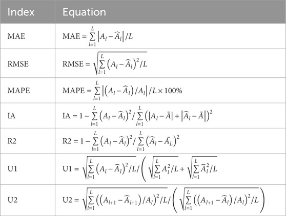
TABLE 2. Index of valuation.

4.1.2.1 Correlation strength

The Spearman correlation coefficient (Spearman), also called Spearman’s rank correlation coefficient, is used to measure the correlation between two variables. Spearman proposed a different method, using the order of the data size instead of the numerical value itself. The correlation strength indicators can show the superiority of the innovative ensemble prediction model.

4.1.2.2 Forecasting effectiveness

Prediction efficiency is an essential means of measuring prediction performance. Generally, the evaluation criteria for prediction efficiency are first calculated as an absolute percentage error. Then, the mean and variance of absolute percentage error are used to obtain first-order forecasting effectiveness (FE1) and second-order forecasting effectiveness (FE2).

4.1.2.3 Forecasting stability

Besides prediction efficiency, prediction stability is a significant criterion for evaluating model performance and can be used to evaluate ensemble models. The stability of the prediction is generally measured by the variance of the prediction error (VAR). The smaller the value VAR, the more stable the prediction.

4.1.2.4 Statistical significance

The modified form of the Diebold-Mariano test (MDM) is used to determine whether there are significant differences between different data sets and whether the results of the ensemble prediction model are significantly different from those of other models.

4.2 Data description

To make accurate predictions about carbon emission prices, publicly available carbon trading data from the U.S. Intercontinental Exchange on the investing website were selected for this article. Looking at the classification of external factors affecting carbon emissions, it is clear that energy is the most important factor affecting the carbon trading price selected in this article. Therefore, gas, fuel oil, crude oil, and ethanol data from the same investment website were selected for this article. The impact of gas on carbon emissions is captured as MIDAS-α, while the impact of fuel oil, crude oil, and ethanol on carbon emissions are referred to as MIDAS-β, MIDAS-γ, and MIDAS-δ, respectively.

All five datasets contain high-frequency (daily) and low-frequency (weekly) price data, with weekly carbon trading prices being the target of the prediction in this article. To improve the experiments of the prediction in this article, a total of 900 weekly carbon emission price data are divided into three parts: The first part is a training set to train each sub-model to obtain prediction results, with a total of 720 data; the second and third parts contain a total of 180 data; the second part is the validation set to determine the optimal sub-model, with a total of 135 data points; the third part is the test set to test the error size between the actual value and the test, with a total of 45 data.

Because the weekly dataset is fixed in time, this article considers controlling the start and end times of the training, validation, and testing datasets to ensure that each mixing factor consistently affects the carbon trading price. A total of 4,500 data were obtained by filling in the missing data. To increase the accuracy of the data, 900 data were obtained by processing and completing some outlier data of weekly carbon trading prices. In this paper, a mixed-frequency (MF) example of weekly carbon dioxide emissions trading prices and daily heating oil prices and a common-frequency (CF) example of weekly carbon dioxide emissions trading prices and weekly natural gas prices are selected as typical examples, as shown in Figure 2 and Table 3. The statistical characteristics tables and the two-sample Kolmogorov-Smirnov test table for all datasets are shown below and indicate that the p-value is 0.0000. Therefore, it can be assumed that a significant difference exists between the different factors, and using them as factors affecting carbon prices to achieve good results is reasonable.

FIGURE 2

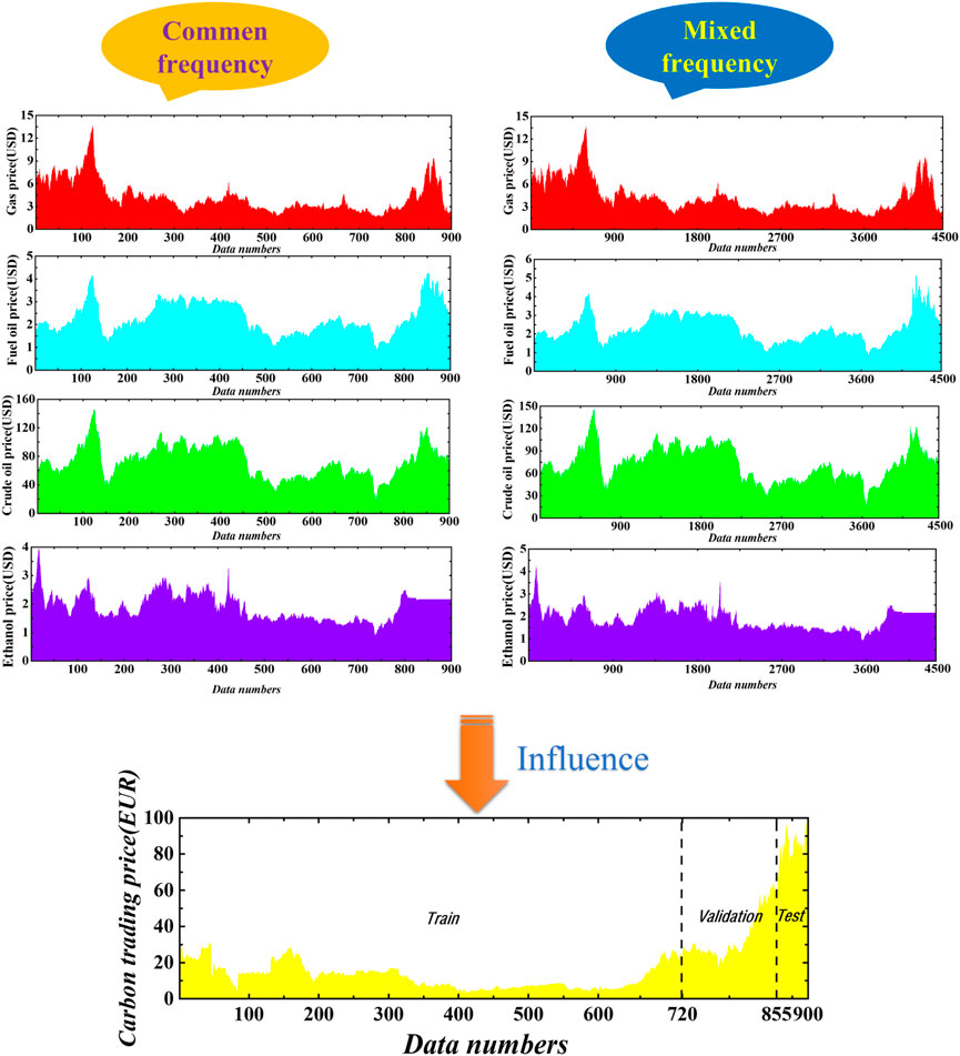
FIGURE 2. Dataset with CF and MF.

TABLE 3

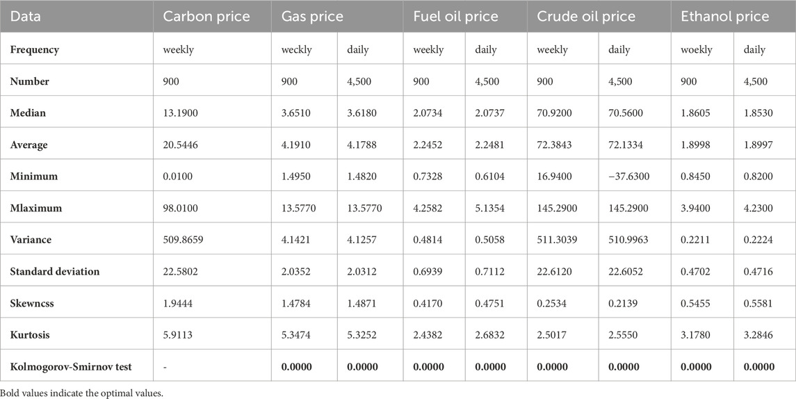
TABLE 3. Statistical characteristics of the dataset.

4.3 Experimental design

Four experiments were conducted in this article to demonstrate the rationality and effectiveness of carbon price prediction. In experiment 1, the lag order is set from 1 to 6, and the CEI index is used to evaluate the optimal lag order of the different submodels and select the optimal submodel in the CF models. The MF models require the simultaneous discussion of the lag order of x and y. In the second experiment, the preprocessed submodels were compared with the corresponding submodels, confirming the superiority and effectiveness of SA-VMD decomposition. In the third experiment, the prediction effects and errors of the submodels CF and MF and the effects and errors of the preprocessed submodels CF and MF were compared. The comparison of the ensemble model with the previous submodels shows the effectiveness and superiority of the ensemble method, as shown in Experiment 4.

4.4 Experiment 1: establishment of optimal submodel

In carbon price prediction, it is crucial to select the optimal submodel to obtain a satisfactory ensemble model in the future. Therefore, this article considers comparisons based on data preprocessing techniques and determining the optimal lag order by CEI indicators to determine the optimal submodel. Specifically, this article selects the optimal index by creating an MF-MIDAS model with lag orders y from 1 to 6, lag orders x from 7 to 42, and intervals of 7. Moreover, the three machine learning models with the CF all have lag orders from 1 to 8, and the specific prediction results are shown in the table. In addition, the optimal submodel is the one that has the lowest CEI value. The CEI results corresponding to the different lag orders are shown in Figures 3, 4 below. Due to the consideration that the lag order table is too large, the table has been moved to the Supplementary.

(1) For the mixed frequency MIDAS model, as shown in the table in the appendix, the optimal AR-MIDAS model is determined by taking values from 1 to 6 and 7 to 42 for different lag orders y and x, respectively, using the lowest CEI value and polynomial comparison. For example, in MIDAS-α without data pre-processing, it can be found that when ylag = 5, xlag = 35, and Legendre polynomials is selected as the polynomial, CEI achieves the lowest value of 3.3849, which is superior to other lag orders and polynomial selection. Therefore, this model is the optimal MIDAS-α sub-model at this time. Similarly, it can be seen that MIDAS-β, MIDAS-γ, and MIDAS-δ are the optimal sub-models when ylag = 5 and xlag = 7, and the polynomials are Legendre polynomials. For the AR-MIDAS model after data preprocessing: ylag = 3, xlag = 35 when Legendre polynomials is selected as the polynomial, it is the optimal SA-VMD-MIDAS-α submodel; ylag = 6, xlag = 35, when the polynomial is Legendre polynomials, it is the optimal SA-VMD-MIDAS-β submodel; ylag = 6, xlag = 35, when the polynomial is Legendre polynomials, it is the optimal SA-VMD-MIDAS-γ submodel; When ylag = 6, xlag = 35, and the polynomial is a Beta polynomial, it is the optimal SA-VMD-MIDAS-δ submodel.

(2) For artificial intelligence models of the same frequency, as shown in the table in the appendix, three optimal SA-VMD-CF models (SA-VMD-KELM, SA-VMD-RNN, SA-VMD-GRNN) and three optimal CF models (KELM, RNN, GRNN) were obtained by comparing the order of 1–6 lags. For example, by comparing the CEI values corresponding to different lag orders, it is easy to see that when the lag order is 2, the SA-VMD-KLEM submodel with data preprocessing has the lowest CEI value of 2.6602, which is better than the results of others. This means that a lag order of 2 is the optimal SA-VMD-KELM submodel. Similarly, the optimal lag orders for KELM, RNN, and GRNN are 1, 1, and 5, respectively. Similarly, SA-VMD-RNN and SA-VMD-GRNN, which have undergone data preprocessing, obtain the optimal submodels when the lag orders are 6 and 6, respectively.

FIGURE 3

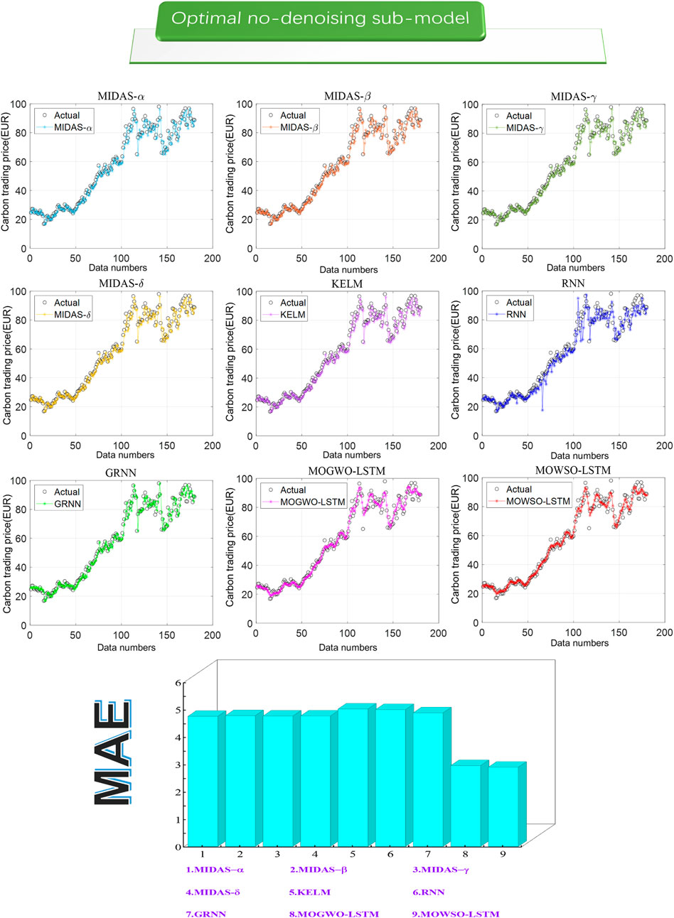
FIGURE 3. Optimal submodel and ensemble model.

FIGURE 4

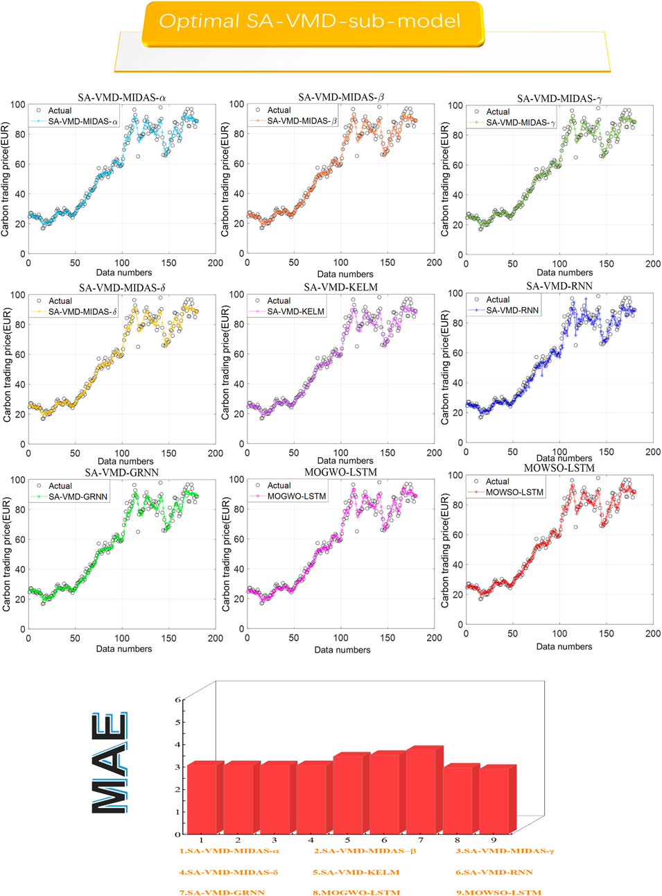
FIGURE 4. Optimal submodel with data preprocessing and ensemble model.

Remark: Experiment 1 selects the optimal MIDAS and machine learning models by comparing the CEI index, laying a solid foundation for future ensemble prediction. The experimental results indicate the optimal lag order of the optimal submodel.

4.5 Experiment 2: comparison of sub-models with SA-VMD and sub-models

This experiment verifies the superiority of data preprocessing and the advantages of SA-VMD decomposition by contrasting the submodels with corresponding submodels after data preprocessing. We compared the various indicators of the optimal submodel obtained in Experiment 1 and compared the indicators of the submodel with or without data preprocessing as shown in Figure 5 and Tables 4, 5 below:

(1) The first comparison between the submodels and the corresponding submodels after data preprocessing shows that data preprocessing plays a crucial role in predicting the mixing of carbon emission prices. As shown in the table, all the blending submodels without data preprocessing have lower indicators than those decomposed with SA-VMD, indicating that the submodels decomposed with SA-VMD outperform the corresponding submodels in various aspects of prediction. For example, the MAPE indicator of MIDAS-α is 5.7765, while the MAPE indicator of the SA-VMD-MIDAS-α model is only 3.7497; After data preprocessing, the MAE decreased from 4.7597 to 3.0673, and the MDM test p-value of 0.0000 also fully proves the superiority of SA-VMD-MIDAS-α compared to MIDAS-α. Similarly, it can be found that SA-VMD-MIDAS-β, SA-VMD-MIDAS-γ, and SA-VMD-MIDAS-γ all outperform their corresponding sub-models in terms of predictive indicators.

(2) In the second comparison, the superiority and importance of SA-VMD decomposition in the CF artificial intelligence deep learning submodels can be established by comparing the corresponding submodels without SA-VMD decomposition and SA-VMD decomposition. As shown in the table, the submodels with SA-VMD technology outperform the corresponding submodels in predicting indicators in all aspects. This indicates that the submodels decomposed by SA-VMD are superior to the corresponding submodels. For example, the MAPE indicator of the KELM model is 6.0841, while the MAPE indicator of SA-VMD-KLEM is only 4.1554. The MAE and RMSE decreased from 5.0294 to 6.0285 to 3.4535 and 4.3557, respectively. The result of the MDM test also proves the superiority of SA-VMD-KELM over KELM. Similarly, both SA-VMD-RNN and SA-VMD-GRNN can outperform their corresponding submodels in predicting indicators.

FIGURE 5

FIGURE 5. Model with preprocessing and without preprocessing.

TABLE 4

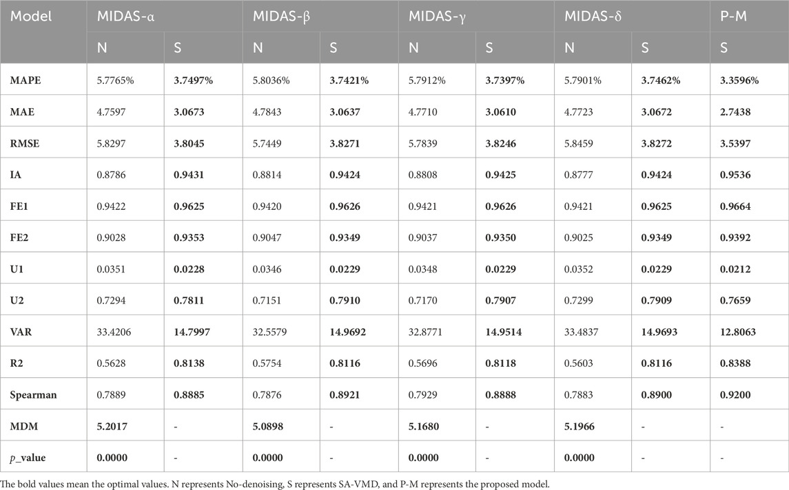
TABLE 4. Result of MIDAS model SA-VMD-MIDAS model.

TABLE 5

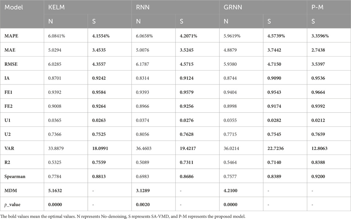
TABLE 5. Result of ANN model SA-VMD-ANN model.

Remark: Experiment 2 compared the evaluation indicators of the submodels after data preprocessing with the corresponding submodels, and the results showed that the submodels after SA-VMD was significantly better in prediction than the corresponding sub-model.

4.6 Experiment 3: comparison of the MF and CF models

This experiment demonstrates the important role and irreplaceability of MF in carbon emission price prediction through comparison. Also, it demonstrates the rationality and necessity of using MF sub-models in prediction. The result is listed in Table 6.

TABLE 6

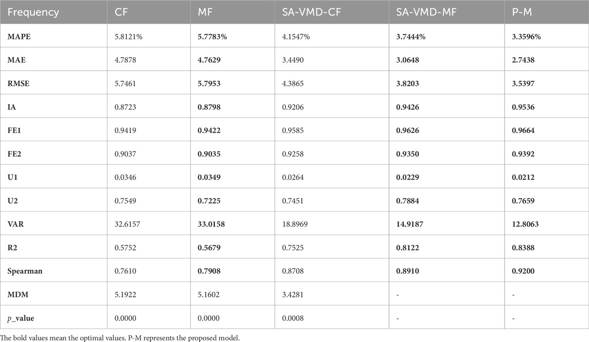
TABLE 6. Result in the experiment 3.

(1) In the first comparison, several MF and CF submodels were averaged to obtain the forecasting results, as shown in Table 6 below. From the comparison of the CF model and the MF model, almost all the evaluation indices of the mixture model are better than the initial frequency, proving the mixing and common frequency prediction’s effectiveness and necessity. For example, the MAPE of the common frequency model is 5.8121, while it is reduced to 5.7783 for the mixed frequency model, and the MAE is also reduced from 4.7878 to 4.7629. The results show that adding a mixed model can improve prediction ability and accuracy.

(2) In the second comparison, it can be seen that the preprocessed SA-VMD-MF is significantly better than SA-VMD-CF, and all indicators of the mixing model after VMD decomposition are significantly better than the same frequency model after SA-VMD decomposition. For example, the MAPE of the SA-VMD-CF model has decreased from 4.1547 to 3.7444 of the SA-VMD-MF model, while the MAE has also decreased from 3.4490 to 3.0648. The comparison results prove the effectiveness of the mixing model and once again prove the progressiveness and rationality of the preprocessing.

Remark: Experiment 3 compared the prediction performance between common frequency and mixed frequency submodels and found that the mixed frequency model outperformed the common frequency model, demonstrating the necessity and importance of incorporating a mixed frequency model in carbon trading price prediction.

4.7 Experiment 4: comparison of ensemble models

To verify the superiority of the ensemble technology and fully exploit the efficiency of Deep Learning, a new ensemble strategy MOWSO-LSTM model is developed in this experiment. As a generalization of the basic RNN model, the LSTM can effectively overcome the RNN gradient explosion problem and is robust to noise. This paper measures the importance of the new integration methods for carbon price prediction by comparing the ensemble effects of MOALO-LSTM, MOGWO-LSTM, and MOWSO-LSTM. At the same time, the comparison of each optimal sub-model and the ensemble model also shows the progressiveness and effectiveness of the ensemble strategy. The comparison between the proposed model and other ensemble models and the comparison results of the optimal submodels and the proposed model are shown in Tables 7, 8. The result is listed in Figures 6–9.

TABLE 7

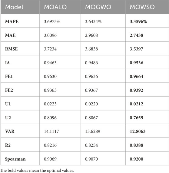
TABLE 7. The comparison of ensemble models.

TABLE 8

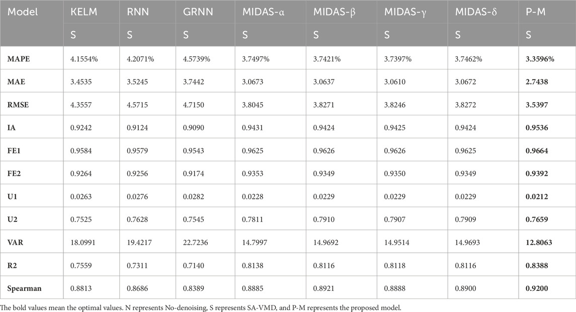
TABLE 8. The results of ensemble model and other optimal submodels.

FIGURE 6

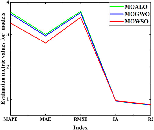
FIGURE 6. Comparison of multi-objective algorithms.

FIGURE 7

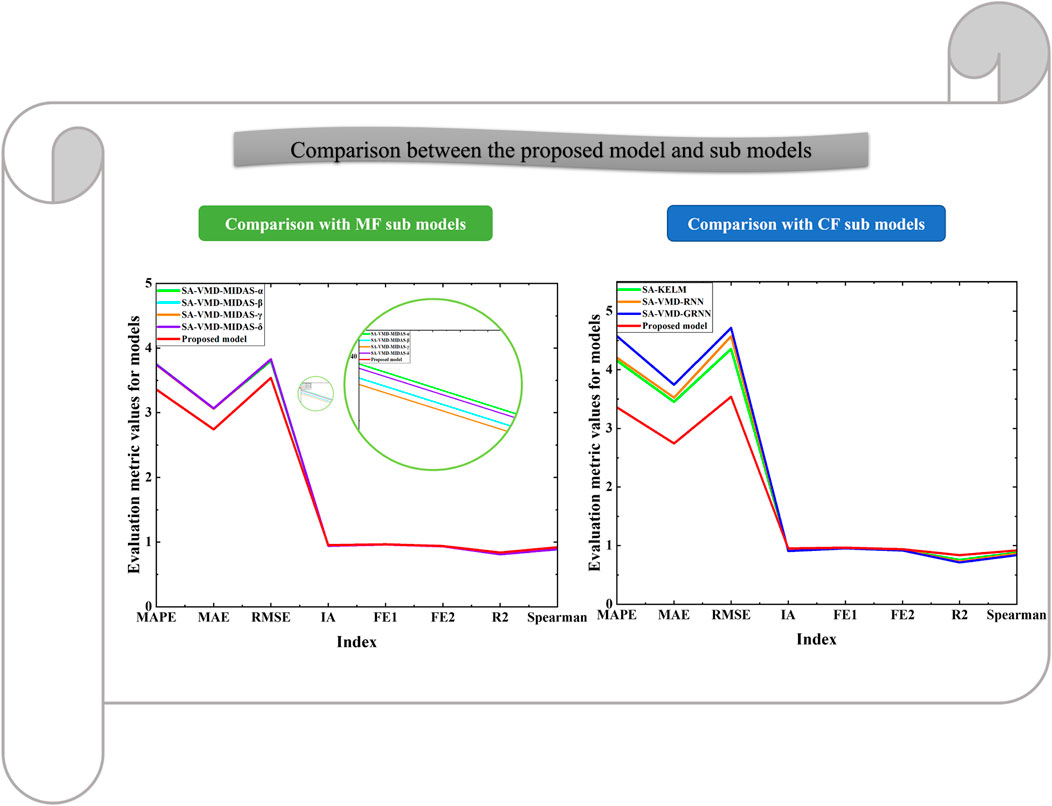
FIGURE 7. Comparison between the proposed model and sub models.

FIGURE 8

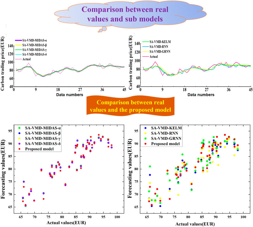
FIGURE 8. Comparison between real values and models.

FIGURE 9

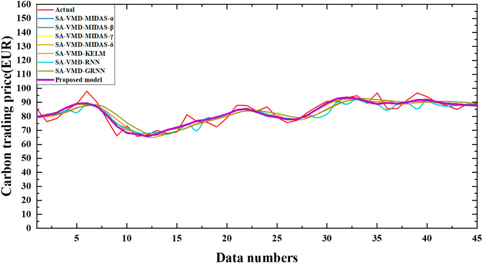
FIGURE 9. Comparison between models.

(1) The first comparison shows that each indicator of the new ensemble strategy model is superior to other ensemble models by comparing the errors of the three ensemble models, which demonstrates the advantages of the new ensemble strategy. For example, the MAPE of MOALO-LSTM is 3.6975, while the MAPE of MOWSO-LSTM is only 3.3596. At the same time, MAE decreased from 3.0096 to 2.7438, and RMSE fell from 3.7234 to 3.5397. MOWSO-LSTM also outperforms other ensemble strategies MOGWO-LSTM in every indicator. The experiment fully proves that the ensemble strategy MOWSO-LSTM is necessary and can enhance the prediction of carbon trading prices.

(2) The second comparison compares the optimal artificial intelligence submodels and MF with the new ensemble model after preprocessing the data. It can be seen that each indicator of MOWSO-LSTM is superior to all the individual sub-models, which once again proves the effectiveness and superiority of the ensemble strategy. For example, the MAPE of the optimal submodel of KELM after data preprocessing is 4.1554, the MAPE of MIDAS-γ after data preprocessing is 3.7397, and the MAPE of MOWSO-LSTM is only 3.3596. The MAPE index of the proposed model improved by 28.3526% compared to machine learning models. The MAE of MOWSO-LSTM is 2.7438, and the IA is 0.9536, both of which are superior to the optimal submodels. The MAE index of the proposed model improved by 30.2597% compared to machine learning models. At the same time, the other indicators of the new ensemble model are also prominent to a single optimal submodel. The experiment once again clearly illustrates the progressiveness of the new ensemble strategy and provides an effective method to improve the price forecasting ability of carbon trading.

Remark: In Experiment 4, by comparing the LSTM model based on the deep learning strategy using different multi-objective optimization algorithms, the proposed model is superior to other multi-objective ensemble models and any optimal sub-model.

5 Conclusion

The current prediction of carbon trading prices faces complexities in terms of temporal distribution characteristics and uncertainties, making it challenging to achieve high accuracy. This study introduces the concept of mixed frequencies into the carbon trading price prediction field to consider the temporal distribution characteristics of carbon trading prices better to overcome these challenges. A novel integrated prediction method is developed to reduce uncertainties and improve prediction results. Specifically, this research includes a data preparation module, a mixed-frequency modeling module based on attention mechanism, and a machine learning module. The mixed-frequency and machine learning module consists of three CF (continuous frequency) models and 4 MF (mixed frequency) models, and the optimal sub-models are determined based on proposed evaluation criteria to consider the temporal distribution characteristics of carbon trading prices sufficiently. Lastly, an ensemble module based on the LSTM model is developed, taking advantage of the strengths of deep learning to reduce parameter uncertainties in carbon trading price prediction. A multi-objective algorithm is used to find the optimal solution for LSTM parameters, resulting in the proposed model. The proposed model outperforms all individual sub-models in various indicators. For example, the MAPE of the best sub-models, SA-VMD RNN and SA-VMD MIDAS2, are 4.2071% and 3.7421%, respectively, while the MAPE of MOWSO-LSTM is only 3.5327%. The FE1 and FE2 of the proposed model are 0.9664 and 0.9392, which are better than each best sub-model.

Some specific innovations and conclusions can be listed as follows:

(a)By successfully incorporating mixed frequencies, the prediction of carbon trading prices is improved, and the predictive performance is enhanced. Experimental results show that adequately utilizing mixed-frequency data helps reduce price prediction errors and provides a more comprehensive consideration of the temporal distribution characteristics than a single machine learning model.

(b)The best sub-models are preprocessed using SA-VMD. The optimal solution for the varying patterns is successfully searched through iterations, and various mode functions and central frequencies are continuously updated to obtain multiple mode functions with specific bandwidths. Comparing the data preprocessing sub-models with their corresponding sub-models demonstrates the necessity of data preprocessing in price prediction, avoiding potential parameter uncertainties in data preprocessing.

(c)New evaluation criteria based on machine learning and mixed-frequency modules are proposed, which can fully utilize various evaluation indicators to obtain the optimal sub-models. These evaluation criteria measure the performance among different models and help select the optimal sub-models, avoiding potential parameter uncertainties during the sub-model prediction process.

(d)Based on the optimal sub-models, a deep learning-based multi-objective optimization ensemble module is proposed to enhance the results of carbon trading price prediction. It is found that MOWSO optimizes three parameters of the LSTM ensemble forecaster, avoiding parameter uncertainties that may occur in ensemble prediction.

In conclusion, the proposed novel ensemble prediction model can be used to investigate better the temporal distribution characteristics and uncertainties of carbon trading prices. It considers and overcomes the issues of data preprocessing decomposition techniques and parameter uncertainties in ensemble models while fully utilizing the temporal distribution characteristics of carbon trading prices at different frequencies. The results also demonstrate that the model has more potential and value compared to existing models, and these methods can also be applied to other prediction problems. However, there are still some limitations and prospects in this study. Specifically, although the static ensemble model performs better than each sub-model, a dynamic ensemble based on Bayesian methods may yield even better results. Furthermore, the current iteration of dynamic ensemble weights is mainly based on single accuracy evaluation indicators. Further research can explore multi-objective optimization methods to update weights, simultaneously considering dynamic ensemble weights’ accuracy and stability. In addition, regarding data preprocessing, this study only considers the closeness in the direction of vector values when determining the number of decomposition modes using the self-attention mechanism of VMD without considering the approximation in magnitude. There is still room for further optimization, and other data preprocessing methods, such as EMD and EWT, may also be applicable depending on the data’s frequency and temporal distribution characteristics. Different data preprocessing methods for data with different frequencies and temporal distribution characteristics may yield better results.

Data availability statement

Publicly available datasets were analyzed in this study. This data can be found here: https://cn.investing.com/.

Author contributions

ZL: Investigation, Writing–original draft, Writing–review and editing. JL: Writing–review and editing. LL: Writing–review and editing.

Funding

The author(s) declare financial support was received for the research, authorship, and/or publication of this article. This work was funded by the Guangxi Science and Technology Project (No. GuikeAD21220082), Guangxi Key Laboratory of Big Data in Finance and Economics (No. FED2202), Guangxi First-class Discipline Statistics Construction Project (Nos. 2022SXYB08, TJYLXKDSJ 2022A02), Guangxi Natural Science Foundation (Nos. 2020GXNSFAA159014, 2021GXNSFAA220114).

Conflict of interest

The authors declare that the research was conducted in the absence of any commercial or financial relationships that could be construed as a potential conflict of interest.

Publisher’s note

All claims expressed in this article are solely those of the authors and do not necessarily represent those of their affiliated organizations, or those of the publisher, the editors and the reviewers. Any product that may be evaluated in this article, or claim that may be made by its manufacturer, is not guaranteed or endorsed by the publisher.

Supplementary material

The Supplementary Material for this article can be found online at: https://www.frontiersin.org/articles/10.3389/fenrg.2023.1341881/full#supplementary-material

References

Akhtar, M. S., and Feng, T. (2022). Detection of malware by deep learning as cnn-lstm machine learning techniques in real time. Symmetry 14, 2308. doi:10.3390/sym14112308

CrossRef Full Text | Google Scholar

Alhakami, H., Kamal, M., Sulaiman, M., Alhakami, W., and Baz, A. (2022). A machine learning strategy for the quantitative analysis of the global warming impact on marine ecosystems. Symmetry 14, 2023. doi:10.3390/sym14102023

CrossRef Full Text | Google Scholar

Alsulami, A. A., Abu Al-Haija, Q., Alqahtani, A., and Alsini, R. (2022). Symmetrical simulation scheme for anomaly detection in autonomous vehicles based on lstm model. Symmetry 14, 1450. doi:10.3390/sym14071450

CrossRef Full Text | Google Scholar

Altan, A., Karasu, S., and Bekiros, S. (2019). Digital currency forecasting with chaotic meta-heuristic bio-inspired signal processing techniques. Chaos, Solit. Fractals 126, 325–336. doi:10.1016/j.chaos.2019.07.011

CrossRef Full Text | Google Scholar

Borup, D., Rapach, D. E., and Schütte, E. C. M. (2023). Mixed-frequency machine learning: nowcasting and backcasting weekly initial claims with daily internet search volume data. Int. J. Forecast. 39, 1122–1144. doi:10.1016/j.ijforecast.2022.05.005

CrossRef Full Text | Google Scholar

Braik, M., Hammouri, A., Atwan, J., Al-Betar, M. A., and Awadallah, M. A. (2022). White shark optimizer: a novel bio-inspired meta-heuristic algorithm for global optimization problems. Knowledge-Based Syst. 243, 108457. doi:10.1016/j.knosys.2022.108457

CrossRef Full Text | Google Scholar

Chai, F., Li, Y., Zhang, X., and Chen, Z. (2023). Daily semiparametric garch model estimation using intraday high-frequency data. Symmetry 15, 908. doi:10.3390/sym15040908

CrossRef Full Text | Google Scholar

Chang, T., Hsu, C.-M., Chen, S.-T., Wang, M.-C., and Wu, C.-F. (2023). Revisiting economic growth and co2 emissions nexus in taiwan using a mixed-frequency var model. Econ. Analysis Policy 79, 319–342. doi:10.1016/j.eap.2023.05.022

CrossRef Full Text | Google Scholar

Chen, Y., Dodwell, T., Chuaqui, T., and Butler, R. (2023). Full-field prediction of stress and fracture patterns in composites using deep learning and self-attention. Eng. Fract. Mech. 286, 109314. doi:10.1016/j.engfracmech.2023.109314

CrossRef Full Text | Google Scholar

Chullamonthon, P., and Tangamchit, P. (2023). Ensemble of supervised and unsupervised deep neural networks for stock price manipulation detection. Expert Syst. Appl. 220, 119698. doi:10.1016/j.eswa.2023.119698

CrossRef Full Text | Google Scholar

Dong, Y., Wang, J., Wang, R., and Jiang, H. (2023). Accurate combination forecasting of wave energy based on multiobjective optimization and fuzzy information granulation. J. Clean. Prod. 386, 135772. doi:10.1016/j.jclepro.2022.135772

CrossRef Full Text | Google Scholar

Dragomiretskiy, K., and Zosso, D. (2013). Variational mode decomposition. IEEE Trans. signal Process. 62, 531–544. doi:10.1109/tsp.2013.2288675

CrossRef Full Text | Google Scholar

Du, L., Gao, R., Suganthan, P. N., and Wang, D. Z. (2022). Bayesian optimization based dynamic ensemble for time series forecasting. Inf. Sci. 591, 155–175. doi:10.1016/j.ins.2022.01.010

CrossRef Full Text | Google Scholar

Emam, W., and Tashkandy, Y. (2023). Modeling the amount of carbon dioxide emissions application: new modified alpha power weibull-x family of distributions. Symmetry 15, 366. doi:10.3390/sym15020366

CrossRef Full Text | Google Scholar

Fallahi, A., Shahidi-Zadeh, B., and Niaki, S. T. A. (2023). Unrelated parallel batch processing machine scheduling for production systems under carbon reduction policies: nsga-ii and mogwo metaheuristics. Soft Comput. 27, 17063–17091. doi:10.1007/s00500-023-08754-0

CrossRef Full Text | Google Scholar

Gallardo-Antolín, A., and Montero, J. M. (2021). An auditory saliency pooling-based lstm model for speech intelligibility classification. Symmetry 13, 1728. doi:10.3390/sym13091728

CrossRef Full Text | Google Scholar

Gao, C., Zhang, N., Li, Y., Lin, Y., and Wan, H. (2023). Adversarial self-attentive time-variant neural networks for multi-step time series forecasting. Expert Syst. Appl. 231, 120722. doi:10.1016/j.eswa.2023.120722

CrossRef Full Text | Google Scholar

Gao, R., Du, L., Duru, O., and Yuen, K. F. (2021). Time series forecasting based on echo state network and empirical wavelet transformation. Appl. Soft Comput. 102, 107111. doi:10.1016/j.asoc.2021.107111

CrossRef Full Text | Google Scholar

Gao, X., Wang, J., and Yang, L. (2022). An explainable machine learning framework for forecasting crude oil price during the covid-19 pandemic. Axioms 11, 374. doi:10.3390/axioms11080374

CrossRef Full Text | Google Scholar

Ghysels, E., and Valkanov, R. (2004). The midas touch: mixed data sampling regression models. Cirano Work. Pap. 5, 512–517.

Google Scholar

Guan, S., and Zhao, A. (2017). A two-factor autoregressive moving average model based on fuzzy fluctuation logical relationships. Symmetry 9, 207. doi:10.3390/sym9100207

CrossRef Full Text | Google Scholar

Guo, Y., Guo, J., Sun, B., Bai, J., and Chen, Y. (2022). A new decomposition ensemble model for stock price forecasting based on system clustering and particle swarm optimization. Appl. Soft Comput. 130, 109726. doi:10.1016/j.asoc.2022.109726

CrossRef Full Text | Google Scholar

Han, M., Ding, L., Zhao, X., and Kang, W. (2019). Forecasting carbon prices in the shenzhen market, China: the role of mixed-frequency factors. Energy 171, 69–76. doi:10.1016/j.energy.2019.01.009

CrossRef Full Text | Google Scholar

Hao, X., Liu, Y., Pei, L., Li, W., and Du, Y. (2022). Atmospheric temperature prediction based on a bilstm-attention model. Symmetry 14, 2470. doi:10.3390/sym14112470

CrossRef Full Text | Google Scholar

Hao, Y., and Tian, C. (2020). A hybrid framework for carbon trading price forecasting: the role of multiple influence factor. J. Clean. Prod. 262, 120378. doi:10.1016/j.jclepro.2020.120378

CrossRef Full Text | Google Scholar

He, W., Xie, Y., Lu, H., Wang, M., and Chen, H. (2020). Predicting coronary atherosclerotic heart disease: an extreme learning machine with improved salp swarm algorithm. Symmetry 12, 1651. doi:10.3390/sym12101651

CrossRef Full Text | Google Scholar

Hochreiter, S., and Schmidhuber, J. (1997). Long short-term memory. Neural Comput. 9, 1735–1780. doi:10.1162/neco.1997.9.8.1735

PubMed Abstract | CrossRef Full Text | Google Scholar

Huang, G.-B., Zhou, H., Ding, X., and Zhang, R. (2011). Extreme learning machine for regression and multiclass classification. IEEE Trans. Syst. Man, Cybern. Part B Cybern. 42, 513–529. doi:10.1109/TSMCB.2011.2168604

PubMed Abstract | CrossRef Full Text | Google Scholar

Huang, G.-B., Zhu, Q.-Y., and Siew, C.-K. (2006). Extreme learning machine: theory and applications. Neurocomputing 70, 489–501. doi:10.1016/j.neucom.2005.12.126

CrossRef Full Text | Google Scholar

Huang, Y., Dai, X., Wang, Q., and Zhou, D. (2021). A hybrid model for carbon price forecasting using garch and long short-term memory network. Appl. Energy 285, 116485. doi:10.1016/j.apenergy.2021.116485

CrossRef Full Text | Google Scholar

James, N., and Menzies, M. (2022). Global and regional changes in carbon dioxide emissions: 1970–2019. Phys. A Stat. Mech. Its Appl. 608, 128302. doi:10.1016/j.physa.2022.128302

CrossRef Full Text | Google Scholar

Jiang, W., and Yu, Q. (2023). Carbon emissions and economic growth in China: based on mixed frequency var analysis. Renew. Sustain. Energy Rev. 183, 113500. doi:10.1016/j.rser.2023.113500

CrossRef Full Text | Google Scholar

Karasu, S., and Altan, A. (2022). Crude oil time series prediction model based on lstm network with chaotic henry gas solubility optimization. Energy 242, 122964. doi:10.1016/j.energy.2021.122964

CrossRef Full Text | Google Scholar

Karasu, S., Altan, A., Bekiros, S., and Ahmad, W. (2020). A new forecasting model with wrapper-based feature selection approach using multi-objective optimization technique for chaotic crude oil time series. Energy 212, 118750. doi:10.1016/j.energy.2020.118750

CrossRef Full Text | Google Scholar

Lahiri, K., and Yang, C. (2022). Boosting tax revenues with mixed-frequency data in the aftermath of covid-19: the case of New York. Int. J. Forecast. 38, 545–566. doi:10.1016/j.ijforecast.2021.10.005

CrossRef Full Text | Google Scholar

Li, X., Zhang, X., and Li, Y. (2022). High-dimensional conditional covariance matrices estimation using a factor-garch model. Symmetry 14, 158. doi:10.3390/sym14010158

CrossRef Full Text | Google Scholar

Lian, J., Liu, Z., Wang, H., and Dong, X. (2018). Adaptive variational mode decomposition method for signal processing based on mode characteristic. Mech. Syst. Signal Process. 107, 53–77. doi:10.1016/j.ymssp.2018.01.019

CrossRef Full Text | Google Scholar

Lin, Y., Liao, Q., Lin, Z., Tan, B., and Yu, Y. (2022). A novel hybrid model integrating modified ensemble empirical mode decomposition and lstm neural network for multi-step precious metal prices prediction. Resour. Policy 78, 102884. doi:10.1016/j.resourpol.2022.102884

CrossRef Full Text | Google Scholar

Medsker, L. R., and Jain, L. (2001). Recurrent neural networks. Des. Appl. 5, 64–67. doi:10.1007/978-1-4842-6513-0_8

CrossRef Full Text | Google Scholar

Niu, X., Wang, J., Wei, D., and Zhang, L. (2022). A combined forecasting framework including point prediction and interval prediction for carbon emission trading prices. Renew. Energy 201, 46–59. doi:10.1016/j.renene.2022.10.027

CrossRef Full Text | Google Scholar

Park, J., Yi, D., and Ji, S. (2020). Analysis of recurrent neural network and predictions. Symmetry 12, 615. doi:10.3390/sym12040615

CrossRef Full Text | Google Scholar

Son, G., Kwon, S., and Park, N. (2019). Gender classification based on the non-lexical cues of emergency calls with recurrent neural networks (rnn). Symmetry 11, 525. doi:10.3390/sym11040525

CrossRef Full Text | Google Scholar

Song, X., Wang, D., Zhang, X., He, Y., and Wang, Y. (2022). A comparison of the operation of China’s carbon trading market and energy market and their spillover effects. Renew. Sustain. Energy Rev. 168, 112864. doi:10.1016/j.rser.2022.112864

CrossRef Full Text | Google Scholar

Specht, D. F. (1991). A general regression neural network. IEEE Trans. neural Netw. 2, 568–576. doi:10.1109/72.97934

PubMed Abstract | CrossRef Full Text | Google Scholar

Sun, W., and Huang, C. (2020). A novel carbon price prediction model combines the secondary decomposition algorithm and the long short-term memory network. Energy 207, 118294. doi:10.1016/j.energy.2020.118294

CrossRef Full Text | Google Scholar

Taborianski, V. M., and Pacca, S. A. (2022). Carbon dioxide emission reduction potential for low income housing units based on photovoltaic systems in distinct climatic regions. Renew. Energy 198, 1440–1447. doi:10.1016/j.renene.2022.08.091

CrossRef Full Text | Google Scholar

Wang, F., Jiang, J., and Shu, J. (2022a). Carbon trading price forecasting: based on improved deep learning method. Procedia Comput. Sci. 214, 845–850. doi:10.1016/j.procs.2022.11.250

CrossRef Full Text | Google Scholar

Wang, H., Shi, W., He, W., Xue, H., and Zeng, W. (2023). Simulation of urban transport carbon dioxide emission reduction environment economic policy in China: an integrated approach using agent-based modelling and system dynamics. J. Clean. Prod. 392, 136221. doi:10.1016/j.jclepro.2023.136221

CrossRef Full Text | Google Scholar

Wang, J., Cui, Q., and He, M. (2022b). Hybrid intelligent framework for carbon price prediction using improved variational mode decomposition and optimal extreme learning machine. Chaos, Solit. Fractals 156, 111783. doi:10.1016/j.chaos.2021.111783

CrossRef Full Text | Google Scholar

Wang, J., Zhang, H., Li, Q., and Ji, A. (2022c). Design and research of hybrid forecasting system for wind speed point forecasting and fuzzy interval forecasting. Expert Syst. Appl. 209, 118384. doi:10.1016/j.eswa.2022.118384

CrossRef Full Text | Google Scholar

Wang, X., Gao, X., Wang, Z., Ma, C., and Song, Z. (2021). A combined model based on eobl-cssa-lssvm for power load forecasting. Symmetry 13, 1579. doi:10.3390/sym13091579

CrossRef Full Text | Google Scholar

Wang, Y., Li, X., and Liu, R. (2022d). The capture and transformation of carbon dioxide in concrete: a review. Symmetry 14, 2615. doi:10.3390/sym14122615

CrossRef Full Text | Google Scholar

Wichitaksorn, N. (2022). Analyzing and forecasting Thai macroeconomic data using mixed-frequency approach. J. Asian Econ. 78, 101421. doi:10.1016/j.asieco.2021.101421

CrossRef Full Text | Google Scholar

Xia, Y., Wang, J., Zhang, Z., Wei, D., and Yin, L. (2023). Short-term pv power forecasting based on time series expansion and high-order fuzzy cognitive maps. Appl. Soft Comput. 135, 110037. doi:10.1016/j.asoc.2023.110037

CrossRef Full Text | Google Scholar

Xing, Q., Wang, J., Jiang, H., and Wang, K. (2023). Research of a novel combined deterministic and probabilistic forecasting system for air pollutant concentration. Expert Syst. Appl. 228, 120117. doi:10.1016/j.eswa.2023.120117

CrossRef Full Text | Google Scholar

Xu, Q., Liu, S., Jiang, C., and Zhuo, X. (2021). Qrnn-midas: a novel quantile regression neural network for mixed sampling frequency data. Neurocomputing 457, 84–105. doi:10.1016/j.neucom.2021.06.006

CrossRef Full Text | Google Scholar

Yang, H., Li, P., and Li, H. (2022a). An oil imports dependence forecasting system based on fuzzy time series and multi-objective optimization algorithm: case for China. Knowledge-Based Syst. 246, 108687. doi:10.1016/j.knosys.2022.108687

CrossRef Full Text | Google Scholar

Yang, R., Liu, H., and Li, Y. (2023). An ensemble self-learning framework combined with dynamic model selection and divide-conquer strategies for carbon emissions trading price forecasting. Chaos, Solit. Fractals 173, 113692. doi:10.1016/j.chaos.2023.113692

CrossRef Full Text | Google Scholar

Yang, W., Tian, Z., and Hao, Y. (2022b). A novel ensemble model based on artificial intelligence and mixed-frequency techniques for wind speed forecasting. Energy Convers. Manag. 252, 115086. doi:10.1016/j.enconman.2021.115086

CrossRef Full Text | Google Scholar

Yuan, E., and Yang, G. (2023). Sa–emd–lstm: a novel hybrid method for long-term prediction of classroom pm2. 5 concentration. Expert Syst. Appl. 230, 120670. doi:10.1016/j.eswa.2023.120670

CrossRef Full Text | Google Scholar

Zhao, J., Kou, L., Jiang, Z., Lu, N., Wang, B., and Li, Q. (2022). A novel evaluation model for carbon dioxide emission in the slurry shield tunnelling. Tunn. Undergr. Space Technol. 130, 104757. doi:10.1016/j.tust.2022.104757

CrossRef Full Text | Google Scholar