Horizontal well placement optimization based on matrix directional continuous element summation algorithm

During the course of actual oilfield development, judicious selection and design of well placement are paramount due to cost constraints and operating conditions. This paper introduces the Matrix Directional Continuous Elements Summation Algorithm (MDCESA), which is utilized to identify that segment with the largest summation for a given length in a 2D or a 3D matrix. An additional function that accounts for the distance between segments was added when searching for multiple segments to avoid intersections or overlaps between segments. The well placement optimization was transformed into a segment summation on a 3D matrix. Our findings reveal significant advancements in well placement optimization. Employing the MDCESA method, six producers were identified and their production performance was compared against two previously selected producers using a reservoir numerical simulator. The results demonstrated that the wells selected through MDCESA exhibited a substantial improvement in production efficiency. Specifically, there was an 11.6% increase in average cumulative oil production over a 15-year period compared to the wells selected by traditional methods. This research not only presents a significant leap in well placement optimization but also sets a foundation for further innovations in reservoir management and development strategies in offshore oilfields.

1 Introduction

Offshore oilfield development plays a vital role in the global energy supply. Estimates from the United States Geological Survey (USGS), approximately 30 percent of the world’s hydrocarbon resources are located in the oceans, with around 60 percent of the oil and 40 percent of the natural gas located in deep and ultra-deep water areas. Recent advancements in deep-water drilling technologies have rendered the exploitation of these resources feasible, positioning deep-water fields as future pivotal contributors to the augmentation of hydrocarbon production (Rogner, 1997; Zou et al., 2015).

However, oilfield development, especially offshore oil and gas development, is a high-risk, high-investment business model that requires huge capital investments to support complex equipment construction, exploration, drilling, production and transportation (Behrenbruch, 1993; Wang et al., 2019). Therefore, compared with the development of onshore oil fields, the strategic development of offshore oil fields (especially deepwater oil fields) typically prioritizes reservoirs with better physical conditions in order to reduce the development cost, which are characterized by low viscosity, high oil abundance, high porosity and high permeability (Gupta and Grossmann, 2016; 2017). In actual oilfield production, the development strategy of “fewer wells, higher production” is mainly adopted, so for reservoir engineers, reasonable well placement selection and well pattern design are of paramount importance.

The well placement optimization problem is considered a challenging task because it involves numerous static and dynamic factors such as reservoir physical properties, heterogeneity, and fluid flow characteristics (Tavallali et al., 2013; Chen et al., 2018). Finding the optimal well placement requires executing a large number of reservoir simulations, which is computationally intensive, so it is crucial to establish a novel efficient well placement optimization method (Islam et al., 2020). In recent years, many researchers have carried out a large number of studies for the well placement optimization problem, which can be mainly divided into three main categories: 1) reservoir numerical simulation method, 2) reservoir potential/quality map method, and 3) surrogate model based intelligent optimization method.

The first mainstream approach to well placement optimization is reservoir numerical simulation. Reservoir numerical simulation is a very important and widely used tool in oilfield development (Coats, 1982, 12290; Peaceman, 2000; Ertekin et al., 2001; Chen, 2007). It utilizes mathematical models and computational techniques to simulate fluid flow and interactions within the reservoir to predict full reservoir and individual well production performance (Kazemi et al., 1976; Matthäi et al., 2007; Dumkwu et al., 2012).

Reservoir engineers often use the predicted development performance to optimize development plans. Wei et al. (2017) utilized a comprehensive dataset, including seismic data, well logs, and production history, to categorize a super-giant carbonate reservoir into three types (good, medium, and poor), established their distribution patterns, and proposed tailored water flooding plans based on fine-scale geological modeling and reservoir numerical simulation, effectively increasing the estimated ultimate recovery (EUR) by more than 20% compared to natural depletion. Li et al. (2016) introduced a systematic technique combining analytical and numerical production analysis, pressure transient analysis, material balance analysis, and geological analysis to effectively evaluate reservoir properties and forecast production performance of fractured vuggy carbonate gas condensate reservoirs with complex characteristics. Agada et al. (2014) utilized a high-resolution three-dimensional outcrop model of a Jurassic carbonate ramp to perform detailed and systematic flow simulations, demonstrating that reservoir performance and oil recovery in carbonate reservoirs are significantly influenced by small- and large-scale geological features, with subseismic faults and oyster bioherms identified as major controls, and showcased how optimizing well placement and injection fluid can mitigate fluid channelling and enhance oil recovery.

Simulation based method also widely used in well placement optimization. Forouzanfar et al. (2010) developed a two-stage well placement optimization method, employing a gradient-based algorithm with the adjoint method and gradient projection for constraints, effectively determining the optimal number, locations, and rates of water injection and producing wells, while mitigating the effects of pre-specifying well rates and operational reservoir life. Taware et al. (2012) utilized a novel method based on streamline simulation and total time of flight calculations to optimize well placements in a mature offshore carbonate field, outperforming traditional well placement techniques and successfully validating the approach with subsequent field infill drilling. Deng et al. (2010) implemented a comprehensive approach integrating proactive well placement technology, thorough rock physics and petrophysics studies, geomechanical analysis, and real-time interpretation and reservoir simulation, successfully enhancing productivity beyond initial predictions for horizontal wells in the complex offshore field of Bohai Bay. Yu et al. (2015) applied numerical reservoir simulation to model CO₂ injection as a huff-n-puff process in Bakken tight oil reservoirs, revealing that CO₂ molecular diffusion significantly enhances oil recovery, especially in formations with lower permeability, longer fracture half-length, and more heterogeneity, providing valuable insights into the effectiveness and key parameters of CO₂ enhanced oil recovery in unconventional tight oil reservoirs. van Vark et al. (2004) conducted a simulation study evaluating various enhanced oil recovery processes in low permeability carbonate reservoirs in Abu Dhabi, concluding that miscible acid gas injection emerges as the preferable recovery method due to its favorable interaction with native oil, efficient asphaltene dissolution, and advantageous mobility ratio. Al-Fadhli et al. (2019) utilized modeling and simulation to implement the downhole water sink technique with an inverted ESP completion in Greater Burgan Field, achieving increased ultimate oil recovery, mitigated rapid water coning conditions in a high permeability water drive reservoir, and established an optimal development strategy, resulting in a 25% increase in oil production and an 18% reduction in water production over 5 years in the study well.

The second commonly used method of well placement optimization is the reservoir production potential map or quality map method. The reservoir production potential map, also known as a quality map, is a visual graphical tool used to characterize the differences in production potential among various regions of a reservoir. It is usually based on the results of reservoir numerical simulation, and integrates some key reservoir parameters and production data to visualize complex data and help reservoir engineers make more rational decisions.

The concept of the reservoir production potential map was first introduced by da Cruz et al. (1999). Da Cruz et al. (2004) introduced the “quality map” a 2D representation aiding in reservoir management by visualizing reservoir responses and uncertainties. The “quality map” is created by running flow simulations with varied well locations and generating multiple stochastic realizations to capture geological uncertainties, with applications demonstrated across 50 realistic reservoir models.

Some researchers have improved the calculation method of production potential map on the basis of previous studies in order to better characterize the production performance and represent the internal differences of reservoirs. Badru (2003) presented basic and modified quality map approaches which provide a straightforward two-dimensional reservoir representation requiring no simulation runs. The approaches enhanced efficiency of well placement optimization by using the quality map as a preliminary screening tool (Badru and Kabir, 2003). De et al. (2005) developed a faster and reliable methodology for generating quality maps, essential tools in defining and optimizing production strategies, by integrating geological and fluid variables to identify areas with varying production potentials. The effectiveness of this approach is demonstrated using three reservoir models. Liu and Jalali (2006) presented a methodology that transforms standard reservoir models into maps of production potential, guiding the strategic placement of wells across various phases of field development. This approach shows a marked improvement in field recovery factor when compared to traditional fixed spacing approaches. Ding et al. (2014) modified the productivity model to account for the negative effects of bottom water and gas cap on field development, thereby providing a more accurate representation of the production potential in various grid blocks of the reservoir.

Some researchers have combined production potential map and stochastic search algorithms to develop some well placement optimization methods. Chen et al. (2017) employed an analytical formula-based objective function and Cat Swarm Optimization (CSO) algorithm to establish a well placement optimization method, solving the problem of low efficiency in traditional well placement optimization processes that rely on numerical simulators, and significantly accelerating the well placement optimization process. Ding et al. (2019) utilized the Direct Mapping of Productivity Potential (DMPP) technique and Threshold Value of Productivity Potential (TVPP) management strategy in conjunction with Particle Swarm Optimization (PSO), to establish a more efficient well placement optimization process, significantly reducing optimization time while maintaining optimization effectiveness in oil field development. Harb et al. (2020) implemented the black hole particle swarm optimization (BHPSO) method, a hybrid evolutionary optimization technique, for simultaneous well placement optimization in terms of well count, location, type, and trajectory, achieving superior performance compared to the standard PSO with reduced computational requirements.

The third method used for well placement optimization is an artificial intelligence approach based on an surrogate model. Some researchers believe that potential maps and stochastic search algorithms are not always effective in solving well placement optimization problems. Therefore, they look for new ways to establish surrogate models as the basis of optimization algorithms, and data-driven artificial intelligence models are one of them (Liu et al., 2021; Peng et al., 2022; Zhang et al., 2022; Zhong et al., 2022).

Salehian et al. (2022) utilized an ensemble learning of surrogate-models-assisted optimization framework, incorporating Convolutional Neural Network (CNN) and Simultaneous Perturbation Stochastic Approximation (SPSA), to provide diverse and near-optimum well placement solutions with reduced computational cost, achieving superior operational flexibility and computational efficiency compared to conventional methods in the Brugge and Egg field case studies. Moolya et al. (2022) employed a hybrid approach combining surrogate modeling and Multiperiod Mixed-Integer Linear Programming (MILP), alongside a novel methodology of Spatial Aggregation and Disaggregation, to efficiently determine optimal producer locations accounting for surface infrastructure constraints, significantly reducing computational expenses while ensuring maximization of the NPV. Foroud et al. (2012) employed various metamodeling techniques, including 18 different metamodels, and integrated the best performing model with a Genetic algorithm for global optimization search, to efficiently determine the optimal location, direction, and length of a new horizontal well in a mature oil reservoir, resulting in a substantial increase in accumulative oil production and a significant reduction in computation time. Arouri et al. (2022) utilized a surrogate-based well-placement optimization approach, incorporating both analytical and physics-based surrogates with manifold mapping, a multi-fidelity technique, in derivative-free, noninvasive corrections to optimize drilling locations within hydrocarbon reservoirs, demonstrating noticeable computational acceleration and effective well placement in hydrocarbon fields under stringent computing resource constraints. Nasir et al. (2020) developed a hybrid optimization framework named E-MADS, integrating the Enhanced Success History-Based Adaptive Differential Evolution (ESHADE) strategy with a Mesh Adaptive Direct Search (MADS) local pattern search method, and employed a gradient boosting machine learning technique to create a surrogate model, achieving superior performance in the joint optimization of well location and time-varying control for oil fields. Redouane et al. (2019) implemented a hybrid intelligent system combining a Genetic Algorithm (GA), a hybrid constraint-handling strategy, Gaussian Process (GP) surrogate modeling, and an adaptive sampling routine, optimizing well placement in fractured reservoirs with arbitrary well trajectories, complex grids, and various constraints, showcasing high accuracy and efficiency in the challenging real well placement project in El Gassi field, Hassi-Massoud, Algeria. Pouladi et al. (2017) introduced a novel proxy using the Fast Marching Method (FMM) for volumetric pressure approximation to optimize production well placement, achieving satisfactory results with significantly reduced computational costs, demonstrated through application to single and multiple production well placements in standard reservoir models, and comparison with conventional simulator-based methods. Miyagi et al. (2018) applied various variants of the Covariance Matrix Adaptation Evolution Strategy (CMA-ES) with mixed integer support to optimize well placement and injection scheduling in a Carbon dioxide Capture and Storage (CCS) project, discovering that the CMA-ES with step-size lower bound outperformed other variants, showcasing robustness and effectiveness in handling mixed integer programming problems in geologic CO₂ storage optimization. Redouane et al. (2018) developed a hybrid intelligent approach, integrating adaptive space-filling surrogate modeling with an evolutionary algorithm, to optimize well placement under field constraints, resulting in a more accurate, reliable, and efficient solution compared to traditional automatic optimization routines, even with a realistic and complex reservoir model. Hamida et al. (2017) utilized a modified Genetic Algorithm (GA) incorporating a novel “Similarity Operator” for optimal well placement in oil fields, enhancing the solution quality by considering interactions with pre-located wells and geological features, demonstrating robust performance on both the PUNQ-S3 and Brugge field datasets.

Based on the previous literature research we found that there are advantages and disadvantages of these three methods as listed in Table 1. Reservoir numerical simulation is currently the most credible tool for optimization, but its high computational complexity and the need to run a large number of cases when faced with a well optimization problem leads to its low computational efficiency. The optimization method that combines the reservoir production potential map and the stochastic search algorithm offers higher computational efficiency, but this method is generally ineffective in the application of large-scale real reservoir model, which is less practical for the actual production of oilfield. Surrogate model based intelligent optimization method also has similar problems, this method is predominantly applied to theoretical model or mechanism model, and less applied in the actual reservoir model. Currently, the surrogate model unable to fully supplant the reservoir simulation model.

TABLE 1

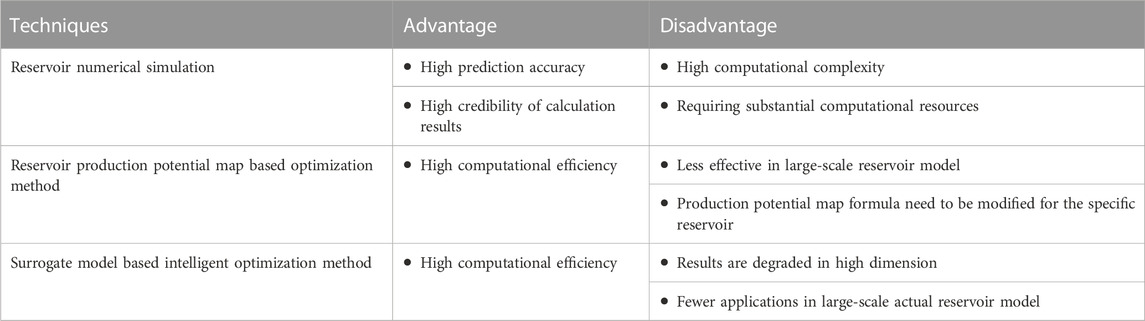
TABLE 1. Comparison of advantages and disadvantages of three main well placement optimization methods.

This paper establishes a fast well placement optimization workflow considering the practical application needs of oilfield production. The basic process involves establishing the Matrix Directional Continuous Elements Summation Algorithm (MDCESA) for 2D planar matrix and 3D spatial matrix, constructing a modified production potential map characterization formula for a specific reservoir, and then using the algorithm to execute a well placement optimization task. This article is divided into the following sections. In Section 2, we introduce the methodology of the Matrix Directional Continuous Elements Summation Algorithm (MDCESA) and reservoir production potential calculation method. Section 3 introduces the application of the proposed method in a actual deep-water reservoir model. The discussion and conclusions are given in Section 4, 5.

2 Methodology

2.1 Matrix directional continuous elements summation algorithm (MDCESA)

The core idea of this method is transforming the horizontal well placement optimization problem into a matrix element summation problem, the reservoir model into a matrix model, and the horizontal section of a horizontal well into a segment of continuous elements of length l.

2.1.1 Calculate max sum of segment

In a two-dimensional planar matrix, this task can be transformed into finding a segment of consecutive points of length l in all possible directions from a given point (m, n), and compute the cumulative value of these sequences to find the sequence with the largest value. This function is defined as “Calculate Max Sum of Segment”.

The principle of “Calculate Max Sum of Segment” is as follows. Assuming that the two-dimensional planar matrix A (Figure 1A) is composed of elements A_mn and dimensions (M × N), where M is the number of rows and N is the number of columns.

FIGURE 1

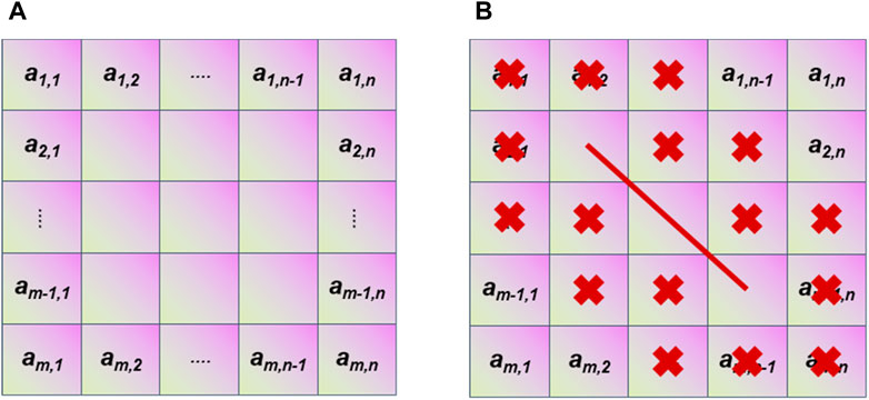
FIGURE 1. Schematic diagram of a two-dimensional planar matrix: (A) a two-dimensional planar matrix; (B) Ignored grid distribution considering the well spacing = 1.

For a given point (m, n) and a direction vector (dx, dy), a segment S is delineated as Eq. 1

$\mathit{S}\left(\mathit{k}\right)={\mathit{A}}_{\mathit{m}+\mathit{k}\cdot \mathit{d}\mathit{x},\mathit{n}+\mathit{k}\cdot \mathit{d}\mathit{y}},\mathit{f}\mathit{o}\mathit{r}\mathbf{0}\le \mathit{k}<\mathit{l}(1)$

where S(k) is the kth element of the segment S, l is the length of the segment.

For a two-dimensional planar matrix, there are eight directions from a given point: [(1, 0), (−1, 0), (0, 1), (0, −1), (1, 1), (1, −1), (−1, 1), (−1, −1)].

The summation for a segment of length l is given by Eq. 2

$\mathit{S}\mathit{u}\mathit{m}\left(\mathit{S}\right)={\displaystyle \sum _{\mathit{k}=\mathbf{0}}^{\mathit{l}-\mathbf{1}}}\mathit{S}\left(\mathit{k}\right)(2)$

The pseudocode for “Calculate Max Sum of Segment” is encapsulated in Algorithm 1. We need to input the matrix and the coordinates of a given point, set the length of the segment, and subsequently computes the sum of the segments in all possible directions and output the value and direction of the max one. The possible cases for each element of the matrix can be calculated through iterative loop traversal.

Algorithm 1.Calculate Max Sum of Segment.

Input: $m,n,l$ (coordinates and length), $matrix$ (MxN matrix)

Output: $\mathit{max}\_sum$ (maximum sum of segment), $\mathit{max}\_dir$ (direction of the segment)

1: function CalculateSegmentSum $\left(m,n,l,matrix\right)$

2:   $lenX\leftarrow \text{number\hspace{0.17em}of\hspace{0.17em}rows\hspace{0.17em}in\hspace{0.17em}matrix}$

3:  $lenY\leftarrow \text{number\hspace{0.17em}of\hspace{0.17em}columns\hspace{0.17em}in\hspace{0.17em}matrix}$

4:  $\mathit{max}\_sum\leftarrow 0$

5:  $\mathit{max}\_dir\leftarrow \text{None}$

6:  $directions\leftarrow \left\{\left(1,0\right),\left(-1,0\right),\left(0,1\right),\left(0,-1\right),\left(1,1\right),\left(1,-1\right),\left(-1,1\right),\left(-1,-1\right)\right\}$

7:  for each $\left(dx,dy\right)$ in $directions$ do

8:   $segment\_sum\leftarrow 0$

9:   for $p\leftarrow 0$ to $l-1$ do

10:    if $0\le m+k\cdot dx<lenX$ and $0\le n+k\cdot dy<lenY$ then

11:      $segment\_sum\leftarrow segment\_sum+matrix\left[m+k\cdot dx\right]\left[n+k\cdot dy\right]$

12:     end if

13:   end for

14:   if $segment\_sum>\mathit{max}\_sum$ then

15:    $\mathit{max}\_sum\leftarrow segment\_sum$

16:    $\mathit{max}\_dir\leftarrow \left(dx,dy\right)$

17:   end if

18:  end for

19:  return $\left(\mathit{max}\_sum,\mathit{max}\_dir\right)$

20: end function

2.1.2 Set horizontal well spacing

Based on the actual situation of oilfield development, well placement optimization needs to consider the distance between wells to preclude the intersection or overlap of wells.

To address this requirement, we introduce a methodology whereby subsequent to the selection of the initial segment, the segment itself along with its adjacent elements are designated as “ignored”. This strategy ensures that the selection of the ensuing segment does not incorporate the constituents of the initial segment. Figure 1 illustrates the basic principle of this approach. The red line represents the horizontal well, and X represents the grid that is ignored when the distance around the horizontal well is 1.

Given a matrix A, a starting point (m, n), a direction vector (dx, dy), the length of segment l, and the well spacing distance, the principle of method is as follows Eq. 3

$\begin{array}{cc}\mathit{A}\mathit{l}\mathit{l}\_\mathit{I}\mathit{g}\mathit{n}\mathit{o}\mathit{r}\mathit{e}\mathit{d}& =\mathit{S}\mathit{e}\mathit{g}\mathit{m}\mathit{e}\mathit{n}\mathit{t}\_\mathit{I}\mathit{g}\mathit{n}\mathit{o}\mathit{r}\mathit{e}\mathit{d}\cup \{\left.\left(\mathit{s}\mathit{x},\mathit{s}\mathit{y}\right)\mid \mathbf{0}\le \mathit{k}<\mathit{l}\right\}\end{array}(3)$

Where, $All\_Ignored$ represents all ignored elements; $Segment\_Ignored$ represents the elements of the previous segment; $\left\{\left(sx,sy\right)\mid 0\le k<l\right\}$ represents the set of elements to be ignored around the previous segment, as shown in Eqs 4, 5

$\mathit{s}\mathit{x}=\mathit{m}+\mathit{k}\cdot \mathit{d}\mathit{x}+\mathit{s}\mathit{u}\mathit{r}\mathit{r}\mathit{o}\mathit{u}\mathit{n}\mathit{d}\_\mathit{d}\mathit{x}(4)$

$\mathit{s}\mathit{y}=\mathit{n}+\mathit{k}\cdot \mathit{d}\mathit{y}+\mathit{s}\mathit{u}\mathit{r}\mathit{r}\mathit{o}\mathit{u}\mathit{n}\mathit{d}\_\mathit{d}\mathit{y}(5)$

Where, $surround\_dx$ and $surround\_dy$ are integers from $-distance$ to $distance$ representing the offsets in the x and y directions when searching around each position $\left(m+k\cdot dx,n+k\cdot dy\right)$.

The pseudocode for Set Horizontal Well Spacing is outlined in Algorithm 2. The “distance” in Algorithm 2 represents the minimum spacing between horizontal wells, by this function we can make sure that horizontal wells will not intersect or overlap with each other. The spacing between them will be greater than value of “distance”.

Algorithm 2.Set Horizontal Well Spacing.

1: Input: $\left(m,n\right)$ - start coordinates of the segment

2:    $l$ - length of the segment

3:    $\left(dx,dy\right)$ - direction vector of the segment

4:    $\text{ignored}$ - current set of ignored points

5:    $\text{distance}$ - surrounding distance to ignore

6: Output: Updated set of ignored points

7: function SetSurroundingToIgnore $\left(m,n,l,dx,dy,\text{ignored},\text{distance}\right)$

8:  $\text{lenX\hspace{0.17em}}\leftarrow \text{number\hspace{0.17em}of\hspace{0.17em}rows\hspace{0.17em}in\hspace{0.17em}matrix}$

9:  $\text{lenY\hspace{0.17em}}\leftarrow \text{number\hspace{0.17em}of\hspace{0.17em}columns\hspace{0.17em}in\hspace{0.17em}matrix}$ ⊳ Iterate over each point in the segment

10: for $k\leftarrow 0$ to $l-1$ do

11:   $\text{currentX\hspace{0.17em}}\leftarrow m+k\cdot dx$

12:   $\text{currentY\hspace{0.17em}}\leftarrow n+k\cdot dy$ ⊳ Iterate over the surrounding area of the current point

13:  for $\text{surround}\_\text{dx\hspace{0.17em}}\leftarrow -\text{\hspace{0.17em}distance\hspace{0.17em}to\hspace{0.17em}distance}$ do

14:   for $\text{surround}\_\text{dy\hspace{0.17em}}\leftarrow -\text{\hspace{0.17em}distance\hspace{0.17em}to\hspace{0.17em}distance}$ do

15:     $\text{surroundX\hspace{0.17em}}\leftarrow \text{currentX}+\text{surround}\_\text{dx}$

16:     $\text{surroundY\hspace{0.17em}}\leftarrow \text{currentY}+\text{surround}\_\text{dy}$ ⊳ Check if the surrounding point is within the matrix boundaries

17:    if $0\le \text{surroundX\hspace{0.17em}}<\text{\hspace{0.17em}lenX}$ and $0\le \text{surroundY\hspace{0.17em}}<\text{\hspace{0.17em}lenY}$ then

18:       $\text{ignored\hspace{0.17em}}\leftarrow \text{ignored}\cup \left\{\left(\text{surroundX},\text{surroundY}\right)\right\}$

19:      end if

20:    end for

21:   end for

22: end for

23: return $\text{ignored}$

24: end function

2.1.3 The framework of the proposed method

The pseudocode delineating the framework of the proposed methodology is encapsulated in Algorithm 3. This framework solves the well placement optimization for a two-dimensional matrix considering horizontal section length and well spacing conditions. Inputting predefined parameters of length of segments (horizontal well length), number of segments (number of horizontal wells), and distance (well spacing), this framework finds the optimal result.

Algorithm 3.Framework of The Proposed Method.

1: Input: matrix, $l$ (length of segments), segments_count (number of segments to find)

2: Output: max_sums (list of maximum sums), max_positions (starting positions of segments), max_directions (directions of segments)

3: function CalculateSegmentSum $\left(m,n,l,\text{matrix}\right)$

4: Compute the sum of segments in all directions from $\left(m,n\right)$ with length $l$

5: return the maximum sum and its direction

6: end function

7: function SetSurroundingToIgnore $\left(m,n,l,dx,dy,\text{ignored},\text{distance}\right)$

8: Mark the surroundings of the segment starting at $\left(m,n\right)$ with direction $\left(dx,dy\right)$ and length $l$ as ignored

9: end function

10: function IsSegmentIgnored $\left(m,n,l,dx,dy,\text{ignored}\right)$

11: Check if the segment starting at $\left(m,n\right)$ with direction $\left(dx,dy\right)$ and length $l$ is in the ignored set

12: return True if ignored, False otherwise

13: end function

14: function FindMaxSegment $\left(\text{matrix},l,m,n,\text{ignored},\text{distance}\right)$

15: Find the segment with the maximum sum in the matrix that is not ignored

16: return the maximum sum, its starting position, and direction

17: end function

18: 

19: procedure Main

20: Load matrix from an Excel file

21: Initialize variables: max_sums, max_positions, max_directions, ignored

22: for segments_count times do

23:   Find the segment with the maximum sum using FindMaxSegment

24:   Add the results to max_sums, max_positions, and max_directions

25:   Update the ignored set using SetSurroundingToIgnore

26: end for

27: Display the results

28: Plot the original matrix and the found segments

29: end procedure

2.1.4 Extending the algorithm to 3D reservoir modeling

The reservoir is a three-dimensional spatial distribution field, and the well placement optimization results based on a two-dimensional planar distribution field are inaccurate. To better simulate the real situation of the reservoir, the application of the proposed framework is extended to a three-dimensional spatial matrix.

The principle of modified Calculate Max Sum of Segment is as follows. Assume that the three-dimensional planar matrix A (Figure 2) has elements A_mnp and dimensions (M × N × P), where M is the number of rows, N is the number of columns, and P is the depth.

FIGURE 2

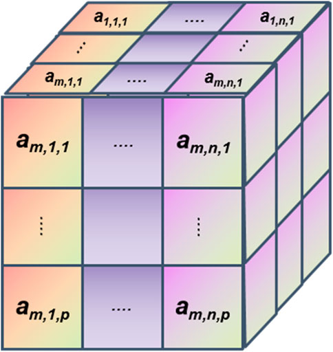
FIGURE 2. Schematic diagram of a three-dimensional matrix.

For a given point (m, n, p) and a direction vector (dx, dy, dz), we can define a segment S as Eq. 6

$\mathit{S}\left(\mathit{r}\right)={\mathit{A}}_{\mathit{m}+\mathit{r}\cdot \mathit{d}\mathit{x},\mathit{n}+\mathit{r}\cdot \mathit{d}\mathit{y},\mathit{p}+\mathit{r}\cdot \mathit{d}\mathit{z}},\mathit{f}\mathit{o}\mathit{r}\mathbf{0}\le \mathit{r}<\mathit{l}(6)$

where S(r) is the rth element of the segment S, l is the length of the segment.

In the 3D matrix, there are 26 possible directions from a given start point, as listed in Table 2.

TABLE 2

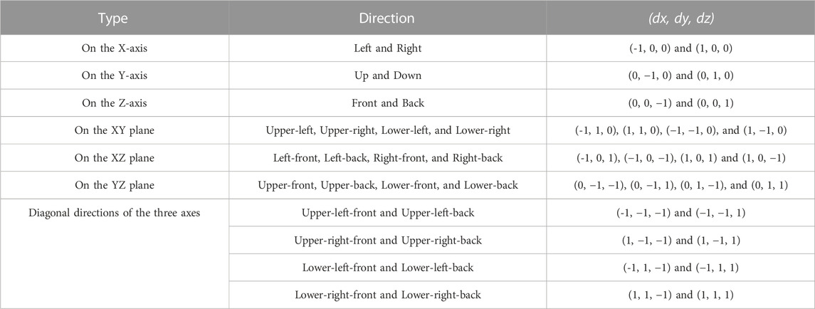
TABLE 2. All possible directions in a 3D matrix starting from a specific point.

The sum of segment of length l as Eq. 7

$\mathit{S}\mathit{u}\mathit{m}\left(\mathit{S}\right)={\displaystyle \sum _{\mathit{r}=\mathbf{0}}^{\mathit{l}-\mathbf{1}}}\mathit{S}\left(\mathit{r}\right)(7)$

The pseudocode for modified Calculate Max Sum of Segment is similar with Algorithm 1. Change the possible directions of the 2D matrix to the possible directions of the 3D matrix (Table 2). In this way, we can find the maximum segment in the 3D matrix for a given length l.

2.2 Application in theoretical models

To validate the proposed method, it is applied to random 2D and 3D matrices. A two-dimensional matrix of dimensions (11 × 11) was synthesized, with each element assigned a random integer ranging from 0 to 100, as illustrated in Figure 3A.

FIGURE 3

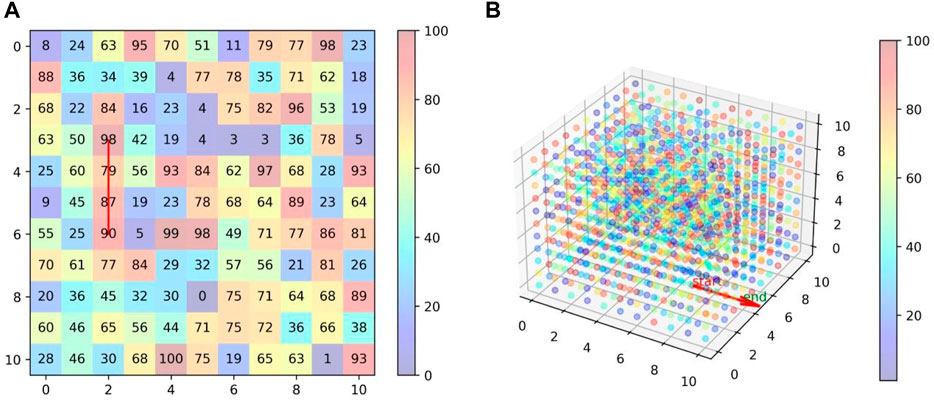
FIGURE 3. Application of MDCESA to random 2D and 3D matrix: (A) Result of 2D matrix; (B) Result of 3D matrix.

The segment length was designated as 4, MDCESA was utilized to systematically assess each element within the matrix. The algorithm computed the sum of the elements spanned by the segment, subsequently identifying the segment’s maximal value, start point, end point, and direction. Similarly, a 3D matrix (11 × 11 × 11) is randomly generated and the same operation is performed using the MDCESA. The visualization results are shown in Figure 3.

In the 2D matrix scenario, value of optimal segment is 354, start position is (3, 2), end position is (6, 2), direction is (1, 0). In the 3D matrix scenario, value of optimal segment is 387, start position is (7, 4, 0), end position is (10, 4, 0), direction is (1, 0, 0).

In order to validate the multi-well optimization considering well spacing, a random two-dimensional matrix with dimensions (20 × 20) was generated for the validation process. Within the MDCESA, the segment length was set at 4, and the well count was set at 4 and 6, respectively. The optimization results are depicted in Figure 4; Table 3. The framework demonstrated robust performance on the random matrix, adeptly identifying optimal segments while ensuring that these segments maintained a separation that met or exceeded a predefined threshold and did not intersect or overlap.

FIGURE 4

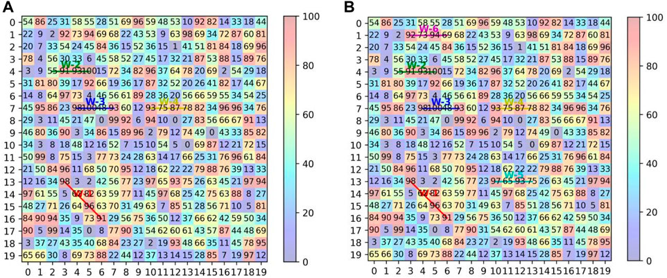
FIGURE 4. Application of MDCESA in random 2D matrix (Considering well spacing): (A) Well count is 4; (B) Well count is 6.

TABLE 3

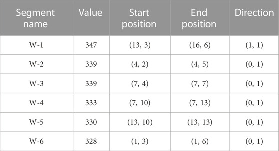
TABLE 3. Results of application of MDCESA in random 2D matrix (Considering well spacing).

2.3 Reservoir production potential

In order to comprehensively consider the influence of reservoir abundance, pore pressure, formation permeability, distance from the boundary and structure position on production capacity, Liu and Jalali (2006) proposed the concept of reservoir production potential based on the study of da Cruz et al. (1999), i.e., the potential oil and gas resource production capacity of the material and energy embedded in the reservoir under the comprehensive consideration of the static and dynamic influencing factors of the reservoir.

The formula for this calculation is outlined as follows:

$\begin{array}{c}{\mathit{J}}_{\mathit{m},\mathit{n},\mathit{p}}\left(\mathit{t}\right)=\left[{\mathit{S}}_{\mathit{o},\mathit{m},\mathit{n},\mathit{p}}\left(\mathit{t}\right)-{\mathit{S}}_{\mathit{o}\mathit{r}}\right]\cdot \left[{\mathit{P}}_{\mathit{o},\mathit{m},\mathit{n},\mathit{p}}\left(\mathit{t}\right)-{\mathit{P}}_{\mathit{min}}\right]\cdot \mathit{ln}{\mathit{K}}_{\mathit{m},\mathit{n},\mathit{p}}\cdot \mathit{ln}{\mathit{r}}_{\mathit{m},\mathit{n},\mathit{p}}\\ \left(\mathit{m}=\mathbf{1,2},\cdots ,{\mathit{n}}_{\mathit{x}};\mathit{n}=\mathbf{1,2},\cdots ,{\mathit{n}}_{\mathit{y}};\mathit{p}=\mathbf{1,2},\cdots ,{\mathit{n}}_{\mathit{z}}\right)\end{array}(8)$

where $J_{m,n,p}\left(t\right)$, $S_{o,m,n,p}\left(t\right)$, and $P_{o,m,n,p}\left(t\right)$ is the production potential, oil saturation, and pressure at the grid (m, n, p) at t time respectively. $S_{or}$ is the residual oil saturation; $P_{\mathit{min}}$ is the minimum well bottom pressure; $K_{m,n,p}$ is the permeability at the grid (m, n, p); $r_{m,n,p}$ is the distance from the grid (m, n, p) to the closest boundary.

In this study, the formula for calculating production potential was tailored to accommodate the specific reservoir type, taking into account the relationships between the target reservoir type, oil-water distribution relationship, structure features, and fluid flow characteristics. This involved an integration of pertinent data, including porosity, permeability, pressure, reservoir thickness, structure elevation, boundary data, and fluid viscosity, to refine the formula, enhancing its specificity and adaptability.

The modified calculation formula is as follows:

$\begin{array}{c}{\mathit{J}}_{\mathit{m},\mathit{n},\mathit{p}}\left(\mathit{t}\right)=\left[{\mathit{S}}_{\mathit{o},\mathit{m},\mathit{n},\mathit{p}}\left(\mathit{t}\right)-{\mathit{S}}_{\mathit{o}\mathit{r}}\right]\cdot \left[{\mathit{P}}_{\mathit{o},\mathit{m},\mathit{n},\mathit{p}}\left(\mathit{t}\right)-{\mathit{P}}_{\mathit{min}}\right]\cdot \mathbf{1}/{\mathit{\mu }}_{\mathit{m},\mathit{n},\mathit{p}}\cdot {\mathit{K}}_{\mathit{m},\mathit{n},\mathit{p}}\cdot {\mathit{\phi }}_{\mathit{m},\mathit{n},\mathit{p}}\cdot \mathit{ln}{\mathit{r}}_{\mathit{m},\mathit{n},\mathit{p}}\cdot \left({\mathit{h}}_{\mathit{m},\mathit{n},\mathit{p}}/\mathit{H}\right)\\ \left(\mathit{m}=\mathbf{1,2},\cdots ,{\mathit{n}}_{\mathit{x}};\mathit{n}=\mathbf{1,2},\cdots ,{\mathit{n}}_{\mathit{y}};\mathit{p}=\mathbf{1,2},\cdots ,{\mathit{n}}_{\mathit{z}}\right)\end{array}(9)$

where ${\mu }_{m,n,p}$ is the viscosity at the grid (m, n, p); ${\phi }_{m,n,p}$ is the porosity at the grid (m, n, p); $h_{m,n,p}$ is the thickness of the formation (the distance from the grid (m, n, p) to the oil-water interface, indicating the effect of the location of the structure on the production potential); $H$ is the distance from the highest point of the reservoir to the oil-water interface.

Moreover, we refrained from applying logarithmic transformation to the permeability values as such a conversion could significantly diminish the influence of permeability on the estimated production potential, a factor particularly critical in low-permeability reservoirs.

The production potential for Reservoir F was estimated utilizing the aforementioned Eqs 8, 9, and the results are visually represented in Figure 5. Figure 5A illustrates the oil saturation distribution of the 3^rd layer of the F reservoir. Figure 5B depicts the computed production potential map, with zones of the model where Net to Gross (NTG) equals zero being purposefully omitted, hence appearing as voids on the map.

FIGURE 5

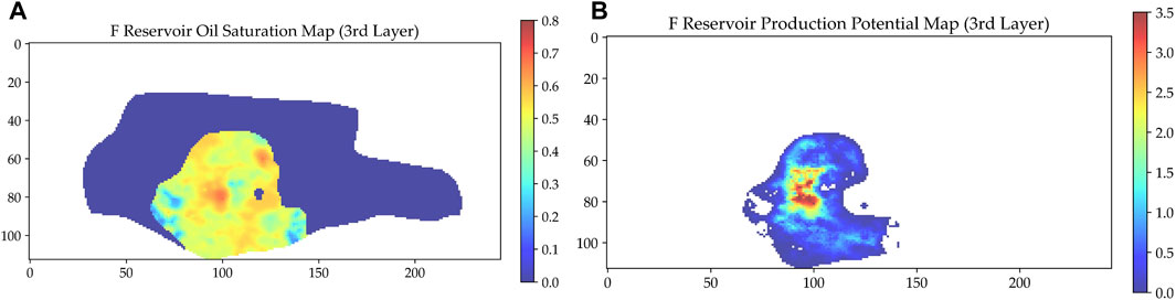
FIGURE 5. Comparison of reservoir oil saturation map and reservoir production potential map: (A) Oil saturation map; (B) Production potential map.

3 Case study

3.1 Workflow

This section aims to apply and validate the proposed MDCESA on the actual offshore reservoir model; the workflow is shown in Figure 6. First, the reservoir model data, formatted in GRDECL, is exported and subjected to data processing. Second, the MDCESA is deployed to optimize well placement based on maps depicting oil saturation and production potential. Finally, the production performance of the optimally positioned wells is corroborated using a reservoir numerical simulator, and the results are benchmarked against those from previously manually chosen wells.

FIGURE 6

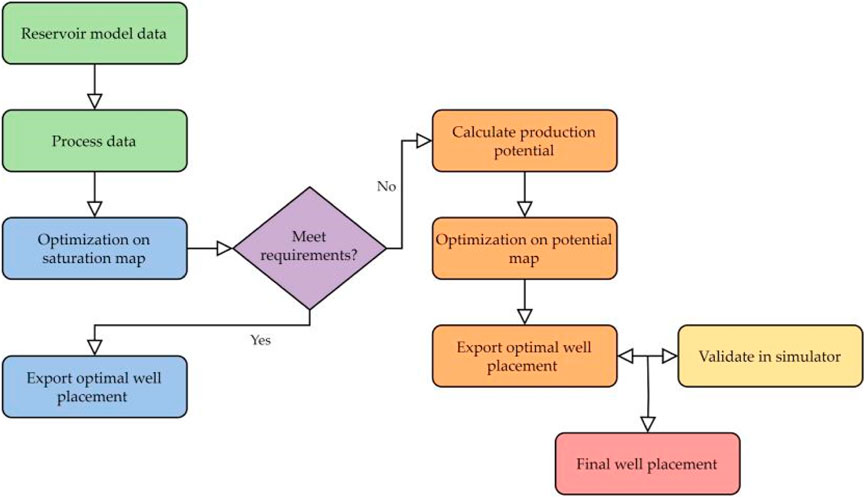
FIGURE 6. Workflow of case study in actual reservoir model.

3.2 Reservoir background

The F reservoir, a deepwater reservoir, is located in the eastern part of the South China Sea, in the northern part of a sag in the Zhujiangkou Basin, where the water depth is about 286 m. The reservoir is a point-reef reservoir developed on the coastal deposit. The sedimentary phases can be categorized as littoral, carbonate plateau, bio-banking, and bio-reef phases in the following order from bottom to top. The depth of the reservoir is from −1802.0 to −1862.5 m, and the reservoir type is low-permeability reef limestone reservoir, with strong non-homogeneity, average porosity of 17.9%–22.3%, average permeability of 5.5–50.1 mD, which belongs to medium-porosity, low-permeability reservoir, and the development of high-angle tectonic fissures.

The fluid of F reservoir is light oil, the viscosity of formation crude oil is 5.5–5.6 mPa∙s, and the fluidity is poor. Considering the lack of natural energy in the limestone reservoir, the reservoir is developed by combining natural energy and artificial water flooding. A total of 10 producers and 3 water injectors are designed, of which most of the producers are long horizontal wells and maximum reservoir contact (MRC) wells in order to maximize the use of reserves and enhance oil recovery. The F reservoir was put into production in September 2022, and a total of 11 wells have been put into production so far.

3.3 Optimization on saturation map

Oil saturation is an important parameter in reservoir development; therefore, the oil saturation map is commonly used to guide well placement optimization. We used MDCESA to optimize on the oil saturation map by setting the number of horizontal wells = 5, horizontal section length = 15 grids (750 m), and minimum well spacing = 4 grids (200 m). Oil saturation map in the 3^rd layer of F reservoir is shown in Figure 7A. From the well placement optimization result (Figure 7B), it can be seen that the ideally sited wells predominantly occupy zones with high oil saturation, congruent with established petrophysical principles.

FIGURE 7

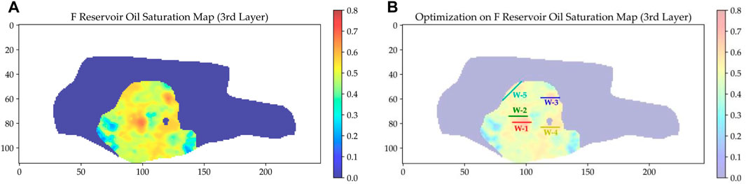
FIGURE 7. Oil saturation map and well placement optimization results: (A) Oil saturation map in the 3^rd layer of F reservoir; (B) Well placement optimization result of F reservoir based on the oil saturation map.

Nevertheless, the optimization derived solely from the oil saturation map overlooked critical factors such as fluid flow capacity, reservoir permeability, reservoir energy, structural complexities, and boundary constraints, all of which significantly impact a well’s production performance. This oversight resulted in the suboptimal placement of well W-5, positioned perilously close to a water body, thereby exposing it to the imminent threat of water breakthrough despite its location in an area of locally high oil saturation.

The reliance on an oil saturation map for well placement is thus deemed inadequate; a more comprehensive approach necessitates the use of a production potential map. This realization underpins the rationale for revising the production potential calculation formula, aiming to integrate all aforementioned factors for a more cogent optimization strategy.

3.4 Optimization on potential map

Facing the challenges of optimization based on oil saturation map, we calculated the production potential map of F reservoir, in which the 3^rd layer is shown in Figure 8A. We set the same parameters for the optimization algorithm: the number of horizontal wells = 5, horizontal section length = 15 grids (750 m), and minimum well spacing = 4 grids (200 m). From the well placement optimization result (Figure 8B), it can be seen that the optimization results are more reasonable compared to the optimization result based on the oil saturation map.

FIGURE 8

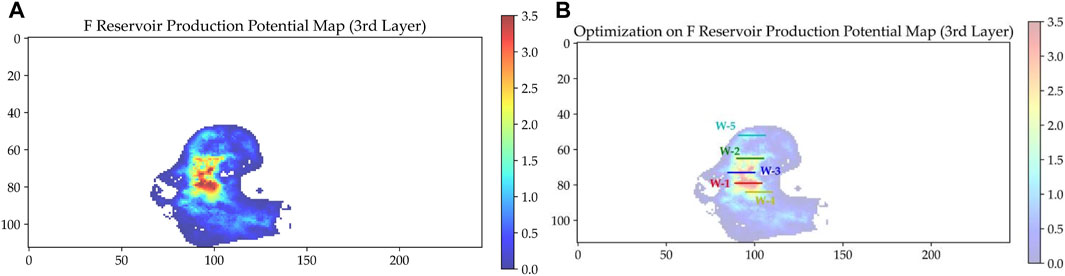
FIGURE 8. Production potential map and well placement optimization results: (A) Production potential map in the 3^rd layer of F reservoir; (B) Well placement optimization result of F reservoir based on the production potential map.

Similarly, we apply MDCESA to the reservoir-wide production potential model for well optimization, setting the number of horizontal wells = 5, horizontal section length = 15 grids (750 m), and minimum well spacing = 4 grids (200 m). The results including the well name, production potential value, start and end positions and direction of each well are shown in Table 4.

TABLE 4

TABLE 4. Results of optimization based on F reservoir production potential model.

3.5 Optimization results evaluation

In order to validate the production performance of the selected horizontal producers, we imported the six producers (W-1, W-2, W-3, W-4, W-5, and W-6) into the reservoir numerical simulator and compared the production of these wells with the previous manually selected wells (A5H and A9H).

Oil production rate and cumulative oil production for these 8 wells are summarized in Figure 9. The performance of the six wells (W-1 through W-6) shows a decreasing sequence that is consistent with their production potential values. The two previously manually planned producers (A5H and A9H) performed worse than the wells selected based on the MDCESA in terms of the length of the plateau, the rate of decline, and the cumulative oil production. Comparing the 15-year cumulative oil production of these wells, the newly selected wells showed an 11.6% increase in average cumulative oil production over the previously selected wells.

FIGURE 9

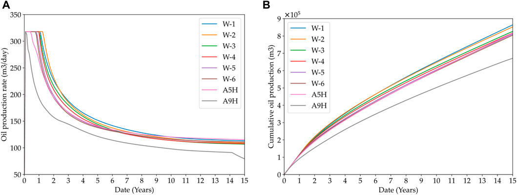
FIGURE 9. Simulated well performance of the selected six producers and the previous manually selected two producers: (A) Oil production rate; (B) Cumulative oil production.

Plotting A5H and A9H on the production potential map (Figures 10B, 11B) shows that both wells are located away from the core area of the production potential map. This locational disadvantage is the primary cause for their diminished production.

FIGURE 10

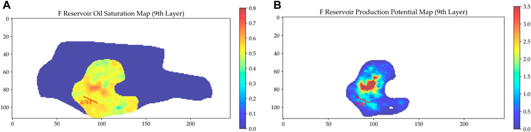
FIGURE 10. Location of the previous manually selected well A5H: (A) Oil saturation map; (B) Production potential map.

FIGURE 11

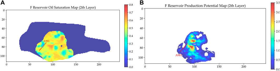
FIGURE 11. Location of the previous manually selected well A9H: (A) Oil saturation map; (B) Production potential map.

The MDCESA method offers superior benefits in terms of precision and efficiency in optimization. Traditional well placement optimization, which rely on geological modeling and iterative reservoir simulation workflows, typically incur substantial time investments—ranging from several days to weeks. In contrast, the MDCESA approach completes the process in a mere fraction of that time, often within minutes to hours.

4 Discussion

The purpose of this research is to develop a novel methodology for quickly obtaining optimal horizontal well placement during the reservoir development. Currently, the traditional workflow of geologic modeling and reservoir numerical simulation consumes a lot of time and computational costs. The application of artificial intelligence techniques that utilize surrogate models and algorithms optimizing multiple parameters has not been extensively realized in practical reservoir scenarios. The utilization of a reservoir production potential map emerges as an effective instrument for guiding the well design and selection process.

The main advantage of the proposed method in this study is that it can quickly identity reasonable well placements, computational efficiency is substantially improved over conventional methods, and the production performance of screened wells is improved, and this method can serve as an important component in the early-stage or mid-stage of the traditional workflow of modeling and simulation to assist in the planning and selection of well placements.

The development of the MDCESA represents a significant step forward in the field of well placement optimization, particularly in the context of offshore oilfield development. The primary objective of this work was to introduce a method that can efficiently identify the most productive segments for well placement in both 2D and 3D matrices. MDCESA stands out in its ability to consider the distance between multiple segments, thus avoiding intersections or overlaps. This approach redefines well placement optimization, transitioning from heuristic and manual selection processes to a more systematic, algorithm-driven method.

While the results obtained using the MDCESA are promising, it is important to acknowledge certain limitations of this method. Firstly, the algorithm’s current form assumes a certain level of uniformity in reservoir characteristics, which may not always be the case in more heterogeneous formations. This could affect the algorithm’s applicability in reservoirs with highly variable geological features. Secondly, the MDCESA, in its current iteration, does not explicitly account for operational constraints such as drilling difficulties or economic factors that could influence well placement decisions. Future versions of the algorithm could be enhanced to include these aspects for a more holistic approach to well placement.

In light of these limitations, future research should focus on enhancing the MDCESA to incorporate a broader range of geological and operational variables. Efforts could also be directed towards testing the algorithm’s effectiveness in different types of reservoirs and under varying operational conditions.

5 Conclusion

In this study, the Matrix Directional Continuous Elements Summation Algorithm (MDCESA) was developed to determine the segment with the maximum value in the 2D and 3D matrices considering the distance between multiple segments. Subsequently, the reservoir production potential calculation formula was modified, which takes into full consideration the static geological characteristics and the dynamic performance of the reservoir. Finally, we transformed the well placement optimization into segment summation on a 3D matrix, and successfully applied MDCESA to actual offshore reservoir development. Our key findings demonstrate that MDCESA significantly enhances well placement decisions, as evidenced by an 11.6% increase in average cumulative oil production over a 15-year period compared to traditional selection methods. In conclusion, the MDCESA offers a novel and effective solution to well placement challenges in offshore oilfields, with promising implications for the future of oil and gas extraction and reservoir management. The specific conclusions are as follows.

1. The establishment of the Matrix Directional Continuous Elements Summation Algorithm (MDCESA) is designed to identify the segment with the highest summation value for a specified length within 2D or 3D matrices. Furthermore, the algorithm has been enhanced by incorporating a feature that accounts for the distance between multiple segments, effectively preventing any intersection or overlap among them.

2. Modified reservoir production potential calculation formula was developed in this study. Compared to the oil saturation map, the production potential map comprehensively characterizes the potential resource production capacity of the material and energy contained in the reservoir, while considering the effects of static and dynamic parameters of the reservoir. The updated formula, which now includes considerations for fluid viscosity, structural elevation, and oil formation thickness, offers a more pragmatic and comprehensive tool for reservoir evaluation.

3. The process of well placement optimization was redefined as a problem of segment summation within a 3D matrix, and the MDCESA was adeptly employed to locate optimal well positions in an actual offshore reservoir based on the production potential map. Six producers were selected using the MDCESA approach and the production performance of each of these six wells and two previously manually selected producers was calculated by using the reservoir numerical simulator. Comparing the 15-year cumulative oil production of these wells, the newly selected wells demonstrated an 11.6% increase in average cumulative oil production over the previously selected wells.

Data availability statement

The original contributions presented in the study are included in the article/supplementary material, further inquiries can be directed to the corresponding author.

Author contributions

RH: Conceptualization, Investigation, Methodology, Validation, Writing–original draft. KW: Conceptualization, Supervision, Writing–review and editing. LL: Supervision, Writing–review and editing. MX: Supervision, Writing–review and editing. JD: Supervision, Writing–review and editing. SF: Supervision, Writing–review and editing. SL: Visualization, Writing–review and editing.

Funding

The author(s) declare financial support was received for the research, authorship, and/or publication of this article. This research was funded by China National Offshore Oil Corporation (CNOOC) Major Science and Technology Project in the 14th Five-Year Plan (Grant No: CNOOC-KJGG2022-0701), and CNOOC (China) Limited Comprehensive Research Project “Key Technology Research for Production Increase of 20 Million Tons in Eastern South China Sea Oilfields” (Grant No: CNOOC-KJ135 ZDXM37SZ03SZ).

Acknowledgments

The authors gratefully acknowledge the support of Nanhai East Petroleum Research Institute. The authors also thank the reviewers for their valuable comments.

Conflict of interest

Authors RH, KW, LL, MX, JD, SF, and SL were employed by Shenzhen Branch of CNOOC Limited.

The authors declare that this study received funding from Shenzhen Branch of CNOOC Limited. The funder was not involved in the study design, collection, analysis, interpretation of data, the writing of this article, or the decision to submit it for publication.

Publisher’s note

All claims expressed in this article are solely those of the authors and do not necessarily represent those of their affiliated organizations, or those of the publisher, the editors and the reviewers. Any product that may be evaluated in this article, or claim that may be made by its manufacturer, is not guaranteed or endorsed by the publisher.

References

Agada, S., Chen, F., Geiger, S., Toigulova, G., Agar, S., Shekhar, R., et al. (2014). Numerical simulation of fluid-flow processes in a 3D high-resolution carbonate reservoir analogue. Pet. Geosci. 20, 125–142. doi:10.1144/petgeo2012-096

CrossRef Full Text | Google Scholar

Al-Fadhli, W., Kurma, R., Kovyazin, D., and Muhammad, Y. (2019). “Modeling and simulation to produce thin layers of remaining oil using downhole water sink technique for improved oil recovery. A case study in greater burgan field,” in Paper presented at the SPE Middle East Oil and Gas Show and Conference, Manama, Bahrain, March, 2019. doi:10.2118/194839-MS

CrossRef Full Text | Google Scholar

Arouri, Y., Echeverría Ciaurri, D., and Sayyafzadeh, M. (2022). A study of simulation-based surrogates in well-placement optimization for hydrocarbon production. J. Petroleum Sci. Eng. 216, 110639. doi:10.1016/j.petrol.2022.110639

CrossRef Full Text | Google Scholar

Badru, O. (2003). Well-placement optimization using the quality map approach. Available at: http://pangaea.stanford.edu/ERE/pdf/pereports/MS/Badru03.pdf (Accessed October 27, 2023).

Google Scholar

Badru, O., and Kabir, C. S. (2003). “Well placement optimization in field development,” in Paper presented at the SPE Annual Technical Conference and Exhibition, Denver, Colorado, October, 2003. doi:10.2118/84191-MS

CrossRef Full Text | Google Scholar

Behrenbruch, P. (1993). Offshore oilfield development planning. J. Petroleum Technol. 45, 735–743. doi:10.2118/22957-PA

CrossRef Full Text | Google Scholar

Chen, H., Feng, Q., Zhang, X., Wang, S., Zhou, W., and Geng, Y. (2017). Well placement optimization using an analytical formula-based objective function and cat swarm optimization algorithm. J. Petroleum Sci. Eng. 157, 1067–1083. doi:10.1016/j.petrol.2017.08.024

CrossRef Full Text | Google Scholar

Chen, H., Feng, Q., Zhang, X., Wang, S., Zhou, W., and Liu, C. (2018). Well placement optimization for offshore oilfield based on Theil index and differential evolution algorithm. J. Petrol Explor Prod. Technol. 8, 1225–1233. doi:10.1007/s13202-017-0403-6

CrossRef Full Text | Google Scholar

Chen, Z. (2007). Reservoir simulation: mathematical techniques in oil recovery. Philadelphia, PA, USA: SIAM/Society for Industrial and Applied Mathematics.

Google Scholar

Coats, K. (1982). Reservoir simulation: state of the art (includes associated papers 11927 and 12290). J. Petroleum Technol. 34, 1633–1642. doi:10.2118/10020-PA

CrossRef Full Text | Google Scholar

da Cruz, P. S., Horne, R. N., and Deutsch, C. V. (1999). “The quality map: a tool for reservoir uncertainty quantification and decision making,” in Paper presented at the SPE Annual Technical Conference and Exhibition, Manama, Bahrain, October, 1999. doi:10.2118/56578-MS

CrossRef Full Text | Google Scholar

Da Cruz, P. S., Horne, R. N., and Deutsch, C. V. (2004). The quality map: a tool for reservoir uncertainty quantification and decision making. SPE Reserv. Eval. Eng. 7, 6–14. doi:10.2118/87642-PA

CrossRef Full Text | Google Scholar

De, A., and Cavalcante Filho, J. S. (2005). “Methodology for quality map generation to assist with the selection and refinement of production strategies,” in Paper presented at the SPE Annual Technical Conference and Exhibition, Dallas, Texas, USA, October, 2005. doi:10.2118/101940-STU

CrossRef Full Text | Google Scholar

Deng, J. M., Liu, P., Zhao, Y. S., Tan, L., Li, G., Yang, B., et al. (2010). “Proactive well placement integrated into a systematical approach enhances productivity in a complex offshore field, Bohai bay,” in Paper presented at the International Oil and Gas Conference and Exhibition in China, Beijing, China, June, 2010. doi:10.2118/131133-MS

CrossRef Full Text | Google Scholar

Ding, S., Jiang, H., Li, J., and Tang, G. (2014). Optimization of well placement by combination of a modified particle swarm optimization algorithm and quality map method. Comput. Geosci. 18, 747–762. doi:10.1007/s10596-014-9422-2

CrossRef Full Text | Google Scholar

Ding, S., Lu, R., Xi, Y., Wang, S., and Wu, Y. (2019). Well placement optimization using direct mapping of productivity potential and threshold value of productivity potential management strategy. Comput. Chem. Eng. 121, 327–337. doi:10.1016/j.compchemeng.2018.11.013

CrossRef Full Text | Google Scholar

Dumkwu, F. A., Islam, A. W., and Carlson, E. S. (2012). Review of well models and assessment of their impacts on numerical reservoir simulation performance. J. Petroleum Sci. Eng. 82 (83), 174–186. doi:10.1016/j.petrol.2011.12.005

CrossRef Full Text | Google Scholar

Ertekin, T., Abou-Kassem, J. H., and King, G. R. (2001). Basic applied reservoir simulation. Richardson, TX, USA: Society of Petroleum Engineers.

Google Scholar

Foroud, T., Seifi, A., and Hassani, H. (2012). Surrogate-based optimization of horizontal well placement in a mature oil reservoir. Petroleum Sci. Technol. 30, 1091–1101. doi:10.1080/10916466.2010.519751

CrossRef Full Text | Google Scholar

Forouzanfar, F., Li, G., and Reynolds, A. C. (2010). “A two-stage well placement optimization method based on adjoint gradient,” in SPE Annual Technical, Florence, Italy, September, 2010. doi:10.2118/135304-MS

CrossRef Full Text | Google Scholar

Gupta, V., and Grossmann, I. E. (2016). “Development planning of offshore oilfield infrastructure,” in Alternative energy sources and technologies: process design and operation. Editor M. Martín (Cham, Germany: Springer International Publishing), 33–87. doi:10.1007/978-3-319-28752-2_3

CrossRef Full Text | Google Scholar

Gupta, V., and Grossmann, I. E. (2017). Offshore oilfield development planning under uncertainty and fiscal considerations. Optim. Eng. 18, 3–33. doi:10.1007/s11081-016-9331-4

CrossRef Full Text | Google Scholar

Hamida, Z., Azizi, F., and Saad, G. (2017). An efficient geometry-based optimization approach for well placement in oil fields. J. Petroleum Sci. Eng. 149, 383–392. doi:10.1016/j.petrol.2016.10.055

CrossRef Full Text | Google Scholar

Harb, A., Kassem, H., and Ghorayeb, K. (2020). Black hole particle swarm optimization for well placement optimization. Comput. Geosci. 24, 1979–2000. doi:10.1007/s10596-019-09887-8

CrossRef Full Text | Google Scholar

Islam, J., Vasant, P. M., Negash, B. M., Laruccia, M. B., Myint, M., and Watada, J. (2020). A holistic review on artificial intelligence techniques for well placement optimization problem. Adv. Eng. Softw. 141, 102767. doi:10.1016/j.advengsoft.2019.102767

CrossRef Full Text | Google Scholar

Kazemi, H., Merrill, L. S., Porterfield, K. L., and Zeman, P. R. (1976). Numerical simulation of water-oil flow in naturally fractured reservoirs. Soc. Petroleum Eng. J. 16, 317–326. doi:10.2118/5719-PA

CrossRef Full Text | Google Scholar

Li, Y., Zhang, J., Liu, Z., Li, B., and Deng, X. (2016). “A systematic technique of production forecast for fractured vuggy carbonate gas condensate reservoirs,” in Paper presented at the SPE Kingdom of Saudi Arabia Annual Technical Symposium and Exhibition, Dammam, Saudi Arabia, April, 2016. doi:10.2118/182776-MS

CrossRef Full Text | Google Scholar

Liu, N., and Jalali, Y. (2006). “Closing the loop between reservoir modeling and well placement and positioning,” in Paper presented at the Intelligent Energy Conference and Exhibition, Amsterdam, The Netherlands, April, 2006. doi:10.2118/98198-MS

CrossRef Full Text | Google Scholar

Liu, W., Zhao, H., Sheng, G., Andy Li, H., Xu, L., and Zhou, Y. (2021). A rapid waterflooding optimization method based on INSIM-FPT data-driven model and its application to three-dimensional reservoirs. Fuel 292, 120219. doi:10.1016/j.fuel.2021.120219

CrossRef Full Text | Google Scholar

Matthäi, S. K., Geiger, S., Roberts, S. G., Paluszny, A., Belayneh, M., Burri, A., et al. (2007). Numerical simulation of multi-phase fluid flow in structurally complex reservoirs. SP 292, 405–429. doi:10.1144/SP292.22

CrossRef Full Text | Google Scholar

Miyagi, A., akimoto, Y., and Yamamoto, H. (2018). “Well placement optimization for carbon dioxide capture and storage via CMA-ES with mixed integer support,” in Proceedings of the Genetic and Evolutionary Computation Conference Companion GECCO ’18, New York, NY, USA, July, 2018, 1696–1703. doi:10.1145/3205651.3205706

CrossRef Full Text | Google Scholar

Moolya, A., Rodríguez-Martínez, A., and Grossmann, I. E. (2022). Optimal producer well placement and multiperiod production scheduling using surrogate modeling. Comput. Chem. Eng. 165, 107941. doi:10.1016/j.compchemeng.2022.107941

CrossRef Full Text | Google Scholar

Nasir, Y., Yu, W., and Sepehrnoori, K. (2020). Hybrid derivative-free technique and effective machine learning surrogate for nonlinear constrained well placement and production optimization. J. Petroleum Sci. Eng. 186, 106726. doi:10.1016/j.petrol.2019.106726

CrossRef Full Text | Google Scholar

Peaceman, D. W. (2000). Fundamentals of numerical reservoir simulation. Amsterdam, Netherlands: Elsevier.

Google Scholar

Peng, X., Rao, X., Zhao, H., Xu, Y., Zhong, X., Zhan, W., et al. (2022). A proxy model to predict reservoir dynamic pressure profile of fracture network based on deep convolutional generative adversarial networks (DCGAN). J. Petroleum Sci. Eng. 208, 109577. doi:10.1016/j.petrol.2021.109577

CrossRef Full Text | Google Scholar

Pouladi, B., Keshavarz, S., Sharifi, M., and Ahmadi, M. A. (2017). A robust proxy for production well placement optimization problems. Fuel 206, 467–481. doi:10.1016/j.fuel.2017.06.030

CrossRef Full Text | Google Scholar

Redouane, K., Zeraibi, N., and Nait Amar, M. (2018). “Automated optimization of well placement via adaptive space-filling surrogate modelling and evolutionary algorithm,” in Paper presented at the Abu Dhabi International Petroleum Exhibition and Conference, Abu Dhabi, UAE, November, 2018. doi:10.2118/193040-MS

CrossRef Full Text | Google Scholar

Redouane, K., Zeraibi, N., and Nait Amar, M. (2019). Adaptive surrogate modeling with evolutionary algorithm for well placement optimization in fractured reservoirs. Appl. Soft Comput. 80, 177–191. doi:10.1016/j.asoc.2019.03.022

CrossRef Full Text | Google Scholar

Rogner, H.-H. (1997). An assessment of world hydrocarbon resources. Annu. Rev. Energy Environ. 22, 217–262. doi:10.1146/annurev.energy.22.1.217

CrossRef Full Text | Google Scholar

Salehian, M., Haghighat Sefat, M., and Muradov, K. (2022). Multi-solution well placement optimization using ensemble learning of surrogate models. J. Petroleum Sci. Eng. 210, 110076. doi:10.1016/j.petrol.2021.110076

CrossRef Full Text | Google Scholar

Tavallali, M. S., Karimi, I. A., Teo, K. M., Baxendale, D., and Ayatollahi, Sh. (2013). Optimal producer well placement and production planning in an oil reservoir. Comput. Chem. Eng. 55, 109–125. doi:10.1016/j.compchemeng.2013.04.002

CrossRef Full Text | Google Scholar

Taware, S., Park, H.-Y., Datta-Gupta, A., Bhattacharya, S., Tomar, A. K., Kumar, M., et al. (2012). “Well placement optimization in a mature carbonate waterflood using streamline-based quality maps,” in Paper presented at the SPE Oil and Gas India Conference and Exhibition, Mumbai, India, March, 2012. doi:10.2118/155055-MS

CrossRef Full Text | Google Scholar

van Vark, W., Masalmeh, S. K., van Dorp, J., Al Nasr, M. A., and Al-Khanbashi, S. (2004). “Simulation study of miscible gas injection for enhanced oil recovery in low permeable carbonate reservoirs in abu dhabi,” in Paper presented at the Abu Dhabi International Conference and Exhibition, Abu Dhabi, United Arab Emirates, October, 2004. doi:10.2118/88717-MS

CrossRef Full Text | Google Scholar

Wang, Y., Estefen, S. F., Lourenço, M. I., and Hong, C. (2019). Optimal design and scheduling for offshore oil-field development. Comput. Chem. Eng. 123, 300–316. doi:10.1016/j.compchemeng.2019.01.005

CrossRef Full Text | Google Scholar

Wei, C., Xiong, L., Zheng, J., and Li, B. (2017). “A comprehensive reservoir characterization and water flooding optimization for different types of reservoir – case study of a giant carbonate reservoir in the Middle East,” in Paper presented at the SPE Symposium: Production Enhancement and Cost Optimisation, Kuala Lumpur, Malaysia, November, 2017. doi:10.2118/189236-MS

CrossRef Full Text | Google Scholar

Yu, W., Lashgari, H. R., Wu, K., and Sepehrnoori, K. (2015). CO2 injection for enhanced oil recovery in Bakken tight oil reservoirs. Fuel 159, 354–363. doi:10.1016/j.fuel.2015.06.092

CrossRef Full Text | Google Scholar

Zhang, K., Wang, X., Ma, X., Wang, J., Yang, Y., Zhang, L., et al. (2022). The prediction of reservoir production based proxy model considering spatial data and vector data. J. Petroleum Sci. Eng. 208, 109694. doi:10.1016/j.petrol.2021.109694

CrossRef Full Text | Google Scholar

Zhong, C., Zhang, K., Xue, X., Qi, J., Zhang, L., Yao, C., et al. (2022). Surrogate-reformulation-assisted multitasking knowledge transfer for production optimization. J. Petroleum Sci. Eng. 208, 109486. doi:10.1016/j.petrol.2021.109486

CrossRef Full Text | Google Scholar

Zou, C., Zhai, G., Zhang, G., Wang, H., Zhang, G., Li, J., et al. (2015). Formation, distribution, potential and prediction of global conventional and unconventional hydrocarbon resources. Petroleum Explor. Dev. 42, 14–28. doi:10.1016/S1876-3804(15)60002-7

CrossRef Full Text | Google Scholar