Research on dynamic robust planning method for active distribution network considering correlation

The universality of load subjects in distribution network brings challenges to the reliability of distribution network planning results. In this paper, a two-stage dynamic robust distribution network planning method considering correlation is proposed. The method evaluates the correlation between random variables using the Spearman rank correlation coefficient, and converts the correlated random variables into mutually independent random variables by Cholesky decomposition and independent transformation; expresses the source-load uncertainty by a bounded interval without distribution, and describes the active distribution network planning as a dynamic zero-sum game problem by combining with the two-phase dynamic robust planning; use the Benders decomposition approach to tackle the issue; mathematical simulation is used to confirm the accuracy and efficacy of the method. The results show that the dynamic robustness planning method of active distribution network taking into account the correlation can accurately simulate the operation of active distribution network with uncertain boundaries, which enhances the reliability and economy of the active distribution network planning results.

1 Introduction

As new energy technology advances, distributed energy has increasingly become a significant component of the energy system (Liu et al., 2016; Xiao et al., 2021). Securing the dependability and safety of distribution network planning and construction is pivotal for the effective rollout of distributed energy accessibility and utilization (Li et al., 2021a; Yang et al., 2022a; Zhang et al., 2022).

In order to plan and coordinate the optimal operation of Distributed Generation (DG) more reasonably, distribution network planning is gradually evolving from the traditional passive mode to the active mode (Chen et al., 2021; Li et al., 2023a). That is to say, the traditional idea of planning passively adapting to the actual operation should be abandoned, and the active decision-making idea of taking operation optimization into consideration and fully tapping the optimization potential in the operation process should be changed (Yang et al., 2018; Li et al., 2020a; Shen et al., 2021).

Research on active distribution network planning addresses uncertainties, such as distributed generation output, as crucial elements (Fang et al., 2022; Xu et al., 2023). The objective is to enhance the resilience, cost-effectiveness, and flexibility of the network while facilitating the widespread integration of renewable energy sources and advancing intelligent power grid development (Yu et al., 2023). Analyzing uncertainties in active distribution network planning is a crucial focus for the future of power grid planning and operation (Yang et al., 2022b; Yu et al., 2022). At present, there are four main methods to study uncertainty: probabilistic programming, Monte Carlo simulation, chance-constrained and robust optimization (Gao et al., 2021; Wang et al., 2021; Li et al., 2023b). Probabilistic planning takes uncertain factors as random variables, and through probabilistic modeling and simulation, the operation results of power grid under different possible scenarios can be obtained, so as to formulate a more robust planning scheme (Tao et al., 2017; Tan et al., 2019; Tan et al., 2020). However, probabilistic planning requires a large amount of data to support, and involves the modeling and calculation of multiple probability distributions, resulting in high computational complexity (Zhou and Zhao, 2013; Zheng et al., 2018). Monte Carlo simulation obtains the operation results of power grid under different scenarios through multiple random sampling calculations, and makes a more comprehensive assessment of power grid planning and decision-making (Peng et al., 2015; Zeng et al., 2015; Chen et al., 2018). However, it is highly dependent on the accuracy of the distribution network uncertainty model and system data, and the data quality directly affects the credibility of the simulation results (Wang et al., 2023; Zhang et al., 2023). Chance constraints regard the possible changes of uncertain factors as “opportunities,” and set corresponding constraints to limit the risk or uncertainty of the planning scheme, to ensure the planning scheme’s robust performance in diverse uncertain conditions (Wang et al., 2019; Su et al., 2021; Zhou et al., 2023). However, as the structure of distribution network becomes more and more complex, the introduction of chance constraints may increase the computational complexity of the optimization problem, which requires more computing resources and time (Liao et al., 2018). Robust optimization, as an optimization method to find the solution with the best stability in the case of considering uncertainty, does not need to know the exact probability distribution, and only needs to use the uncertainty set to describe the uncertainty range of distributed generation output, which is more in line with the practical application requirements (Luo et al., 2018; Li et al., 2020b). Zhang et al. (2019) describes the uncertainty of distributed generation in the form of uncertainty set, and solves the distribution network model through Benders algorithm. Sui et al. (2020) puts forward the idea of discrete uncertain set modeling to obtain more accurate extreme distributed power fluctuation scenarios. Xiao et al. (2022) extends the robust optimization method of distribution network to the new urban distribution network with integrated charging and storage stations and hot spot cogeneration units. As an uncertainty modeling method based on the worst case, robust optimization can effectively guarantee the robustness of the system in the uncertain environment (Fu et al., 2023; Zhu et al., 2023). However, as mentioned above, the existing planning methods based on robust optimization do not consider the correlation between multiple uncertain factors, but treat these uncertain factors as independent events, and then obtain the overall worst scenario by simply adding the worst scenarios of all uncertain factors. However, in the actual operation of active distribution network, some uncertainties are not independent events, but have a certain probability correlation (Li et al., 2021b). In this case, the worst scenario of multiple uncertainties often does not occur at the same time. If this probability correlation is ignored in the process of robust optimization, it will inevitably lead to too conservative planning results. Thereby reducing the effectiveness and economy of the planning decision scheme.

In summary, this paper proposes a two-stage dynamic robust planning method for active distribution networks that considers correlations. Initially, the Spearman rank correlation coefficient is employed to assess the correlation among random variables, and the correlated random variables are transformed into independent random variables by Cholesky decomposition and independent transformation. The polyhedron uncertainty set method is employed to represent source load uncertainty using a distribution-free bounded interval. Combined with the two-stage dynamic robustness programming, the active distribution network planning is described as a dynamic zero-sum game problem between the uncertainty decisions controlled by nature and the human decisions controlled by investors. Finally, the Benders decomposition method is used to solve the problem and the optimal distribution network planning scheme is obtained. The simulation results based on a standard example show that the suggested approach can enhance the reliability and cost-effectiveness of the dynamic distribution system.

This paper makes the following key contributions:

(1) The method for dynamic robust optimization of second order considering correlation is adopted to transform the active distribution network planning problem into a dynamic zero-sum game problem between nature and investors. The planning is designed and corrected by two-stage active decision, and the reliability of the planning results is improved.

(2) The uncertainty of DG and load are represented by undistributed bounded intervals by using polyhedral uncertainty set representation method. By integrating the specifics of the distribution network planning project, we conduct precise simulations of the active distribution network system’s operation under uncertain conditions. This contributes to enhanced reliability and cost-effectiveness in the results of active distribution network planning.

2 Treatment of correlation of random variables and description of its uncertainty

2.1 Treatment of correlation of random variable

There is usually a certain correlation among wind energy, solar power and load in distribution network, and the reliability and economy of distribution network planning scheme will be directly affected by the direct use of historical load data with correlation in distribution network power flow calculation. In view of this, in this study, the Spearman rank correlation coefficient is applied to depict the correlation among random variables. This is complemented by an examination of the traits within the rank correlation matrix, uses Cholesky decomposition and correlation independence transformation method to transform the random variables with correlation into independent random variables, and transforms the historical data with correlation into independent sample combinations.

On this basis, the method of non-parametric kernel density estimation is employed to model the probability density for both photovoltaic output and load. This process determines the marginal probability distribution model through the following specific steps:

1) Correlation processing of original samples of random variables

Historical sample data of random variable PV output and load can be expressed as $\mathbf{H}={\left[h_1,h_2,\cdots ,h_l\right]}^{\mathrm{T}}$, and its correlation coefficient matrix can be expressed as:

${\mathbf{C}}_{\mathrm{H}}=\left[\begin{array}{cccc}1& {\rho }_{h_1{h}_2}& \cdots & {\rho }_{h_1{h}_l}\\ {\rho }_{h_2{h}_1}& 1& \cdots & {\rho }_{h_2{h}_l}\\ ⋮& ⋮& \ddots & \\ {\rho }_{h_l{h}_1}& {\rho }_{h_l{h}_2}& \cdots & 1\end{array}\right](1)$

The correlation coefficient is computed using the following formula:

${\rho }_{h_i{h}_j}=\frac{Cov\left(h_i,h_j\right)}{{\sigma }_{h_i}{\sigma }_{h_j}}=\frac{Cov\left(h_j,h_i\right)}{{\sigma }_{h_i}{\sigma }_{h_j}}={\rho }_{h_j{h}_i}(2)$

In Eq. 2: ${\rho }_{h_i{h}_j}$ and $Cov\left(h_i,h_j\right)$ represent the correlation coefficient and covariance of the random variables $h_i$ and $h_j$. ${\sigma }_{h_i}$ and ${\sigma }_{h_j}$ represent the standard deviations of the random variables $h_i$ and $h_j$, respectively.

The correlation coefficient matrix ${\mathbf{C}}_{\mathrm{H}}$ is a positive definite matrix, which is decomposed by Cholesky to obtain:

${\mathbf{C}}_{\mathrm{H}}=\mathbf{G}{\mathbf{G}}^{\mathrm{T}}(3)$

In Eq. 3: G is the lower triangular matrix, and each element can be solved by the following formula:

$\left\{\begin{array}{ll}{g}_{kk}={\left({\rho }_{h_k{h}_k}-{\displaystyle \sum _{m=1}^{k-1}}{g}_{km}^2\right)}^{1/2},& k=\mathrm{1,2},\cdots ,l\\ g_{ik}=\frac{{\rho }_{h_i{h}_k}-{\displaystyle \sum _{m=1}^{k-1}}{g}_{im}{g}_{km}}{g_{kk}},& i=k+1,\cdots ,l\end{array}\right.(4)$

Formula 2 shows that the correlation coefficient matrix ${\mathbf{C}}_{\mathrm{H}}$ of random variables is a symmetric matrix. Then there is an orthogonal matrix D that can convert the historical sample matrix H with correlation into an uncorrelated sample matrix Q:

$\mathbf{Q}=\mathbf{\text{DH}}(5)$

Considering that the correlation coefficient matrix of the matrix Q is an identity matrix:

$\begin{array}{l}{\mathbf{C}}_Q=\rho \left(\mathbf{Q},{\mathbf{Q}}^{\mathrm{T}}\right)=\rho \left(\mathbf{\text{DH}},{\mathbf{D}}^{\mathrm{T}}{\mathbf{H}}^{\mathrm{T}}\right)\\ =\mathbf{D}\rho \left(\mathbf{H},{\mathbf{H}}^{\mathrm{T}}\right){\mathbf{D}}^{\mathrm{T}}=\mathbf{D}{\mathbf{C}}_{\mathrm{H}}{\mathbf{D}}^{\mathrm{T}}\\ =\mathbf{\text{DG}}{\mathbf{G}}^{\mathrm{T}}{\mathbf{D}}^{\mathrm{T}}=\left(\mathbf{\text{DG}}\right){\left(\mathbf{\text{DG}}\right)}^{\mathrm{T}}=\mathbf{I}\end{array}(6)$

It can be deduced from the above formula, and can be obtained by substituting Formula 5:

$\mathbf{Q}={\mathbf{G}}^{-1}\mathbf{H}(7)$

To sum up, the original sampling data matrix H of random variables with correlation can be represented as the sampling data matrix $\mathbf{Q}={\left[q_1,q_2,\cdots ,q_l\right]}^{\mathrm{T}}$ of random variables with mutual independence.

2) Modeling of PV output and load fluctuation probability density

Using independent PV output and load sample data, this paper employs the non-parametric kernel density estimation method introduced in Xiao et al. (2022) to build the probability density model for PV output and load fluctuation. The process is outlined as follows:

The output of a single photovoltaic unit or the load fluctuation of a single station area were sampled after correlation processing and n samples were obtained. Carry out correlation processing on that original data of the output of a single photovoltaic unit or the load fluctuation of a single substation area and then sample to obtain n samples, that is ${\widehat{q}}_m=\left[{\widehat{q}}_1^m,{\widehat{q}}_2^m,\cdots ,{\widehat{q}}_n^m\right]$, $m\in \left[1,l\right]$. At this time, the probability density function of PV unit output or load fluctuation of single substation area at point $x$ is, and then its nonparametric kernel density estimate is:

$\widehat{f}\left(x\right)=\frac{1}{nh}{\displaystyle \sum _{i=1}^n}K\left(\frac{x-x_i}{h}\right)(8)$

In Eq. 8: $x_i$ is the ith sample data of PV output or load. h is the bandwidth, also known as the smoothing coefficient, which can be obtained according to the empirical formula in Sui et al. (2020). $K\left(\cdot \right)$ is the kernel function.

The selection of kernel functions is diverse, but Sui et al. (2020) points out that different kernel functions have little effect on the accuracy of nonparametric estimation. Therefore, The Gaussian function is commonly utilized as the kernel for estimating the probability density of fluctuations in PV output or load. It can be seen from Formula 8 that the non-parametric kernel density estimation of the probability density model of the output of a single photovoltaic unit or the load fluctuation of a single substation area can be rewritten as:

$\widehat{f}\left(x\right)=\frac{1}{\sqrt{2\pi }nh}{\displaystyle \sum _{i=1}^n}\exp \left[-\frac{1}{2}{\left(\frac{x-x_i}{h}\right)}^2\right](9)$

According to the Formula 9, the probability density function of photovoltaic output $f\left(P_{\text{PVG}}\right)$ and the probability density function of load fluctuation $f\left(P_{\mathrm{L}}\right)$ can be obtained according to the historical photovoltaic output data and load data of the region.

2.2 Determination of uncertain parameter set

The central concept of robust planning is to model the system’s operation under uncertain conditions, based on which the planning and decision-making scheme for the integration of adverse scenarios is formulated, and the key is to construct the uncertain parameter set.

Aiming at the prediction uncertainty of wind power output, photovoltaic power output and load fluctuation in distribution network planning, this paper takes the historical data of wind power output, photovoltaic power output and load as the data base, assumes that all wind turbines, photovoltaic units and loads in the distribution network have the same timing characteristics, incorporates the polyhedron uncertainty set characterization method introduced in Xiao et al. (2022). Wind power output, photovoltaic output, and load uncertainties are individually represented by an undistributed bounded interval denoted as $\mathrm{\Omega }$ .

$\left\{\begin{array}{l}{P}_{p,t,h}^{\mathrm{W}}=S_p^{\mathrm{W}}{\lambda }_h^{\mathrm{W}},P_{p,t,h}^{\mathrm{W},\text{PRE}}=S_p^{\mathrm{W}}{\overline{\lambda }}_h^{\mathrm{W}},\\ {\stackrel{\sim }{P}}_{p,t,h}^{\mathrm{W}}=S_p^{\mathrm{W}}{\stackrel{\sim }{\lambda }}_h^{\mathrm{W}}{P}_{p,t,h}^{\mathrm{P}}=S_p^{\mathrm{P}}{\lambda }_h^{\mathrm{P}},\\ P_{p,t,h}^{\mathrm{P},\text{PRE}}=S_p^{\mathrm{P}}{\overline{\lambda }}_h^{\mathrm{P}},{\stackrel{\sim }{P}}_{p,t,h}^{\mathrm{P}}=S_p^{\mathrm{P}}{\stackrel{\sim }{\lambda }}_h^{\mathrm{P}}\\ P_{p,t,h}^{\mathrm{L}}={\beta }_p{P}_{base}^{\mathrm{L}}{\left(1+\delta \right)}^{t-1}{\lambda }_h^{\mathrm{L}}\\ P_{p,t,h}^{\mathrm{L},\text{PRE}}={\beta }_p{P}_{base}^{\mathrm{L}}{\left(1+\delta \right)}^{t-1}{\overline{\lambda }}_h^{\mathrm{L}}\\ {\stackrel{\sim }{P}}_{p,t,h}^{\mathrm{L}}={\beta }_p{P}_{base}^{\mathrm{L}}{\left(1+\delta \right)}^{t-1}{\stackrel{\sim }{\lambda }}_h^{\mathrm{L}}\end{array}\right.(10)$

In Eq. 10: $S_p^{\mathrm{W}}$ and $S_p^{\mathrm{P}}$ indicate the installed capacity of wind power and photovoltaic units respectively; ${\lambda }_h^{\mathrm{W}}$ and ${\lambda }_h^{\mathrm{P}}$ respectively represent the output of wind power and photovoltaic power of the system at time h (per unit value); ${\overline{\lambda }}_h^{\mathrm{W}}$、 ${\stackrel{\sim }{\lambda }}_h^{\mathrm{W}}$ and ${\overline{\lambda }}_h^{\mathrm{P}}$、 ${\stackrel{\sim }{\lambda }}_h^{\mathrm{P}}$ are the mean value and fluctuation value of wind power and photovoltaic output, respectively (per unit value). $P_{p,t,h}^{\mathrm{W}}$、 $P_{p,t,h}^{\mathrm{W},\text{PRE}}$ and ${\stackrel{\sim }{P}}_{p,t,h}^{\mathrm{W}}$ respectively represent the actual value, predicted value and fluctuation range of wind power output at node p at time h of typical day in year t. $P_{p,t,h}^{\mathrm{P}}$、 $P_{p,t,h}^{\mathrm{P},\text{PRE}}$ and ${\stackrel{\sim }{P}}_{p,t,h}^{\mathrm{P}}$ respectively represent the actual value, predicted value and fluctuation range of wind power output at node p at time h of typical day in year t. ${\lambda }_h^{\mathrm{L}}$ represents the system load (nominal value) at time h, and ${\overline{\lambda }}_h^{\mathrm{L}}$ and ${\stackrel{\sim }{\lambda }}_h^{\mathrm{L}}$ are its average value and fluctuation range respectively; $\delta$ denotes the average annual load growth rate of the system; ${\beta }_p$ is the load rate of system node p; $P_{base}^{\mathrm{L}}$ represents the total system load in the base year; $P_{p,t,h}^{\mathrm{L}}$、 $P_{p,t,h}^{\mathrm{L},\text{PRE}}$ and ${\stackrel{\sim }{P}}_{p,t,h}^{\mathrm{L}}$ represent the actual load value, predicted load value and fluctuation range of node p at time h in year t (the above fluctuation range can be set by planners, and the predicted output value of distributed generation can be equivalent to the average output value of previous years).

$\mathrm{\Omega }=\left\{\begin{array}{l}{\lambda }_h^{\mathrm{W}}\in \left[{\overline{\lambda }}_h^{\mathrm{W}}-{\stackrel{\sim }{\lambda }}_h^{\mathrm{W}},{\overline{\lambda }}_h^{\mathrm{W}}+{\stackrel{\sim }{\lambda }}_h^{\mathrm{W}}\right]\\ {\lambda }_h^{\mathrm{P}}\in \left[{\overline{\lambda }}_h^{\mathrm{P}}-{\stackrel{\sim }{\lambda }}_h^{\mathrm{P}},{\overline{\lambda }}_h^{\mathrm{P}}+{\stackrel{\sim }{\lambda }}_h^{\mathrm{P}}\right]\\ {\lambda }_h^{\mathrm{L}}\in \left[{\overline{\lambda }}_h^{\mathrm{L}}-{\stackrel{\sim }{\lambda }}_h^{\mathrm{L}},{\overline{\lambda }}_h^{\mathrm{L}}+{\stackrel{\sim }{\lambda }}_h^{\mathrm{L}}\right]\\ \frac{{\displaystyle \sum _t^{\mathrm{T}}}{\displaystyle \sum _h^{\mathrm{H}}}{\displaystyle \sum _{p\in {\psi }_{wind}}}\left|\frac{P_{p,t,h}^{\mathrm{W}}-P_{p,t,h}^{\mathrm{W},\text{PRE}}}{{\stackrel{\sim }{P}}_{p,t,h}^{\mathrm{W}}}\right|}{s_{wind}*\mathrm{H}*\mathrm{T}}\\ +\frac{{\displaystyle \sum _t^{\mathrm{T}}}{\displaystyle \sum _h^{\mathrm{H}}}{\displaystyle \sum _{p\in {\psi }_{pvg}}}\left|\frac{P_{p,t,h}^{\mathrm{P}}-P_{p,t,h}^{\mathrm{P},\text{PRE}}}{{\stackrel{\sim }{P}}_{b,t,h}^{\mathrm{P}}}\right|}{s_{pvg}*\mathrm{H}*\mathrm{T}}\\ +\frac{{\displaystyle \sum _t^{\mathrm{T}}}{\displaystyle \sum _h^{\mathrm{H}}}{\displaystyle \sum _{p\in {\psi }_{load}}}\left|\frac{P_{p,t,h}^{\mathrm{W}}-P_{p,t,h}^{\mathrm{W},\text{PRE}}}{{\stackrel{\sim }{P}}_{p,t,h}^{\mathrm{W}}}\right|}{s_{load}*\mathrm{H}*\mathrm{T}}\le \mathrm{\Gamma }\end{array}\right\}(11)$

In Eq. 11: ${\psi }_{wind}$、 ${\psi }_{pvg}$ and ${\psi }_{load}$ represent wind power, photovoltaic and load node sets respectively. $s_{wind}$、 $s_{pvg}$ and $s_{load}$ denote the number of wind power, photovoltaic and load nodes respectively; $\mathrm{H}=24$, representing the number of times of day; t is the planning period; $\mathrm{\Gamma }$ is the conservative index of uncertain set. The larger the value, the larger the fluctuation range, the more uncertainties it contains, and the more conservative the set. At the same time, it also reflects the risk preference of planning decision makers. The larger the value, the more cautious the planners are about the changing range of uncertainties.

3 Second-order cone dynamic robust programming model for distribution network considering demand-side response

3.1 A distribution network planning model incorporating demand-side response

The planning contents include line expansion, location and capacity determination of DG and location and optimal control strategy of DR. Distribution network planning mainly involves equipment investment cost and operation cost. Investment cost is mainly affected by investment decision variables such as equipment model, capacity, quantity and installation selection, while operation cost is not only affected by the above factors, but also dominated by simulation operation variables such as active management process of distribution network. In view of this, the paper explores the influence of user participation in demand-side response on distribution network planning. It establishes a model for active distribution network planning that takes demand-side response into account.

3.1.1 The objective function

In this paper, the demand response of users is considered in distribution network planning, and it is considered that users will adjust their power consumption mode according to their own interests. Usually, the demand side response of users can be achieved in the following two ways: 1) Users reduce load during high-price periods and increase load during low-price periods in the indirect control mode based on time-of-use pricing. This approach aims to achieve peak clipping and valley filling effects; 2) Active load adjustment, the user interrupts the load in the corresponding time period according to the signed contract. In this paper, the second method is adopted, and combined with the distribution network planning method proposed in Zhang et al. (2019), established is an active distribution network planning model that seeks to minimize the combined investment and operational costs:

$\left\{\begin{array}{l}\underset{x^{\text{inv}}{x}^{\text{ope}}}{\min }F\left(x^{\text{inv}},x^{\text{ope}}\right)=C^{\text{inv}}+C^{\text{ope}}\\ \mathrm{s}.\mathrm{t}g\left(x^{\text{inv}}\right)\le 0\\ h\left(x^{\text{inv}},x^{\text{ope}}\right)\le 0\end{array}\right.(12)$

In Eq. 12: $F\left(\cdot \right)$ denotes the objective function; $x^{\text{inv}}$ denotes the investment decision variables of distribution network, including line extension decision, DG location decision and DG capacity decision; $x^{\text{ope}}$ denotes the simulation operation variables of distribution network, which mainly includes natural decision variable $x^{\mathrm{N}}$ and demand side response active management decision variable $x^{\text{inv}}$, including DR location and response electricity quantity; $g\left(\cdot \right)$ denotes investment constraints, usually including equipment investment installation model, quantity, capacity, etc. $h\left(\cdot \right)$ denotes analog operation constraints, including power balance constraints, voltage and current constraints, etc.

3.1.1.1 Investment cost

In this paper, the equipment investment cost $C^{\text{inv}}$ in distribution network planning primarily comprises line expansion and DG investment costs.

1) Line expansion cost $C_{\text{LI}}^{\text{Line}}$ in investment year

$C_{\text{LI}}^{\text{Line}}={\displaystyle \sum _{pq\in {\psi }_{line}}}{e}_{pq}^{\mathrm{L}}{c}_{pq}{l}_{pq}p,q\in {\psi }_{load}(13)$

In Eq. 13: ${\psi }_{line}$ represent a candidate set of lines to be expand; p and q represent load nodes, and $e_{pq}^{\mathrm{L}}$ is a 0–1 variable, indicating whether to build a new line p-q; $c_{pq}$ is the unit investment cost of line p-q; $l_{pq}$ represents the length of the line $p-q$.

2) DG investment cost $C_{\text{LI}}^{\text{DG}}$ in investment year

$C_{\text{LI}}^{\text{DG}}={\displaystyle \sum _{k\in {\psi }_{\text{DG}}}}{\displaystyle \sum _{p\in {\psi }_k}}{e}_p^k{c}^k{S}_p^k(14)$

In Eq. 14: ${\psi }_{\text{DG}}$ represents the collection of distributed generation types to be selected, this paper incorporates both wind power and photovoltaic power generation; ${\psi }_k$ is the set of class k distributed generation installation nodes to be selected; $e_p^k$ is a variable of 0–1, which indicates whether node p is equipped with class k distributed generation; $c^k$ represents the unit capacity investment cost for k-type distributed generation; $S_p^k$ is the installed capacity of class k distributed generation at node p.

Due to the different life cycle of each investment equipment, it is necessary to transfer it to the same planning cycle for investment evaluation. For this reason, the paper transforms the equipment investment cost in the present year into the equivalent annual value for subsequent years. Then the total cost of equipment investment in the same planning period is obtained by converting the equivalent annual value of the cost of equipment investment into the present value and accumulating it.

$\left\{\begin{array}{l}{C}^{\text{inv}}={\displaystyle \sum _{a\in \mathrm{A}}}{\displaystyle \sum _{t=1}^{\mathrm{T}}}{u}_t\lambda C_{\text{LI}}^a\\ u_t=\frac{1}{{\left(1+r\right)}^t}\\ \lambda =\frac{r{\left(1+r\right)}^{\text{EL}}}{{\left(1+r\right)}^{\text{EL}}-1}\end{array}\right.(15)$

In Eq. 15: A represents the set of investment equipment, in this paper $\mathrm{A}=\left\{\text{Line},\text{DG}\right\}$; $C_{\text{LI}}^a$ represents the investment cost of equipment a invested in year LI; $u_t$ is the present value transformation factor; $\lambda$ is the conversion coefficient of equal annual value; EL is the life of equipment; T is the planning period, $\text{LI}\le \mathrm{T}\le \text{LI}+\text{EL}$; r is the social discount rate.

3.1.1.2 Operating cost

The operating cost $C^{\text{ope}}$ primarily encompasses power purchase, power abandonment, network loss, and demand response power costs within the main network.

1) Power purchase cost $C_t^{trans}$ of main grid

$\left\{\begin{array}{l}{C}_t^{trans}={\displaystyle \sum _{h=1}^{\mathrm{H}*365}}{c}^{trans}{P}_{t,h}^{trans}\\ P_{t,h}^{trans}={\displaystyle \sum _{p\in {\psi }_{rest}}}\left(P_{p,t,h}^{trans}-P_{p,t,h}^{\text{DR}}\right)\\ P_{p,t,h}^{trans}=P_{p,t,h}^{\mathrm{L}}-{\displaystyle \sum _{k\in {\psi }_{\text{DG}}}}{P}_{p,t,h}^k\end{array}\right.(16)$

In Eq. 16: $c^{trans}$ indicates the power purchase price of the unit main network; $P_{t,h}^{trans}$ represents the main network purchased electric quantity of the system at time h in the t year; $P_{p,t,h}^{trans}$ represents the main network purchased electric quantity of the node p at time h in the t-th year; $P_{p,t,h}^{\text{DR}}$ denotes the response electric quantity of node p at time h in the t-th year; $P_{p,t,h}^k$ represents the output of k-type distributed generation at node p at time h in year t; ${\psi }_{rest}$ is the node set where there is no power abandonment in the system; $\mathrm{H}=24$, representing the number of hours in a day.

2) Network loss cost $C_t^{loss}$

$\left\{\begin{array}{l}{C}_t^{loss}={\displaystyle \sum _{h=1}^{\mathrm{H}\ast 365}}{\displaystyle \sum _{pq\in {\varphi }_{line}}}{c}^{loss}{P}_{pq,t,h}^{loss}\\ P_{pq,t,h}^{loss}={\left(I_{pq,t,h}\right)}^2{e}_{pq}^{\mathrm{L}}{r}_{pq}\end{array}\right.(17)$

In Eq. 17: $c^{loss}$ represents the average network loss price; ${\varphi }_{line}$ is the system line set; $P_{pq,t,h}^{loss}$ denotes the loss of line $pq$ at t year h time; $r_{pq}$ represents the resistance of line $pq$; $I_{pq,t,h}$ denotes the current of branch $pq$ at time h in year t, which can be obtained by calculating the power flow of distribution network.

3) Power curtailment cost $C_t^{\text{DG}.abandon}$ of distributed generation

$\left\{\begin{array}{l}{C}_t^{\text{DG}.abandon}=C_t^{\mathrm{W}.abandon}+C_t^{\mathrm{P}.abandon}\\ C_t^{\mathrm{W}.abandon}={\displaystyle \sum _{h=1}^{\mathrm{H}\ast 365}}{c}^{\mathrm{W}.abandon}\left(P_{p,t,h}^{\mathrm{W},\text{PRE}}-P_{p,t,h}^{\mathrm{W}}\right)\\ C_t^{\mathrm{P}.abandon}={\displaystyle \sum _{h=1}^{\mathrm{H}\ast 365}}{c}^{\mathrm{P}.abandon}+\left(P_{p,t,h}^{\mathrm{P},\text{PRE}}-P_{p,t,h}^{\mathrm{P}}\right)\end{array}\right.(18)$

In Eq. 18: $c^{abandon}$ represents the unit power abandonment price; $P_{t,h}^{\text{DG}.abandon}$ represents the abandoned electric quantity of the system at the time h in the year t; $P_{p,t,h}^{\text{DG}.abandon}$ indicates the abandoned electric quantity of the distributed power supply at the node p at the time h in the year t.

4) DR electricity cost $C_t^{\text{DR}}$

Where: $C_t^{\text{DR}}$ indicates the DR response price.

The operating costs of the system in each year in the planning cycle are converted into present value costs and accumulated to obtain the total operating costs $C^{\text{ope}}$.

$C^{ope}={\displaystyle \sum _{t=1}^{\mathrm{T}}}{u}_t\left(C_t^{trans}+C_t^{loss}+C_t^{\text{DR}}\right)(19)$

3.1.2 Constraints

3.1.2.1 Equipment investment constraints

1) DG installation capacity constraints

$0\le S_p^k\le S_p^{k.\max }(20)$

In Eq. 20: $S_p^{k.\max }$ represents the upper limit of the installed capacity of the k-type distributed power supply at the node p.

2) DR capacity constraint

$0\le S_p^{\text{DR}}\le P_p^{\mathrm{L}.\max }(21)$

In Eq. 21: $S_p^{\text{DR}}$ refers to the DR capacity signed by the power grid company and the user. $P_p^{\mathrm{L}.\max }$ represents the maximum value of node p load.

3.1.2.2 Security constraints of network operation

1) Network power balance constraints

$\left\{\begin{array}{l}{P}_{p,t,h}=V_{p,t,h}{\displaystyle \sum _{q=1}^{N_{bus}}}{V}_{q,t,h}\left(G_{pq}\cos {\delta }_{pq}+B_{pq}\sin {\delta }_{pq}\right)\\ Q_{p,t,h}=V_{p,t,h}{\displaystyle \sum _{q=1}^{N_{bus}}}{V}_{q,t,h}\left(G_{pq}\sin {\delta }_{pq}-B_{pq}\cos {\delta }_{pq}\right)\\ P_{p,t,h}=P_{p,t,h}^{\mathrm{L}}-{\displaystyle \sum _{k\in {\psi }_{\text{DG}}}}{P}_{p,t,h}^k-P_{p,t,h}^{\text{DR}}\\ Q_{p,t,h}=Q_{p,t,h}^{\mathrm{L}}-{\displaystyle \sum _{k\in {\psi }_{\text{DG}}}}{Q}_{p,t,h}^k-Q_{p,t,h}^{\text{DR}}\\ G_{pq}=\frac{e_{pq}^{\mathrm{L}}{r}_{pq}}{{\left(e_{pq}^{\mathrm{L}}{r}_{pq}\right)}^2+{\left(e_{pq}^{\mathrm{L}}{x}_{pq}\right)}^2}\\ B_{pq}=-\frac{e_{pq}^{\mathrm{L}}{x}_{pq}}{{\left(e_{pq}^{\mathrm{L}}{r}_{pq}\right)}^2+{\left(e_{pq}^{\mathrm{L}}{x}_{pq}\right)}^2}\end{array}\right.(22)$

In Eq. 22: $P_{p,t,h}$ and $Q_{p,t,h}$ respectively represent the injection amount of the active power and the reactive power of the node p at time h in the t-th year; $V_{p,t,h}$ and $V_{q,t,h}$ denote the voltage amplitudes of node p and node q at time h in the t-th year; $x_{pq}$ represents the reactance of the line p-q; $G_{pq}$ and $B_{pq}$ represent the real part and the imaginary part of the nodal admittance matrix, respectively; ${\delta }_{pq}$ represents the phase angle difference of node p and node q.

2) Node voltage and branch current constraints

$\left\{\begin{array}{l}{V}_{p,t,h}^{\min }\le V_{p,t,h}\le V_{p,t,h}^{\max }\\ \left|I_{pq,t,h}\right|\le I_{pq}^{\max }\end{array}\right.(23)$

In Eq. 23: $V_{p,t,h}^{\min }$ and $V_{p,t,h}^{\max }$ respectively the minimum value and the maximum value of the voltage amplitude of the node p at the time h in the year t; $I_{pq}^{\min }$ is the critical overload current of branch $pq$.

3) DR electric quantity constraint

$0\le P_{p,t,h}^{\text{DR}}\le \min \left(S_p^{\text{DR}},P_{p,t,h}^{\mathrm{L}}\right)(24)$

3.2 A two-stage dynamic robust programming model

3.2.1 Second order cone transformation

Active distribution network planning involves a mixed-integer nonlinear programming problem, with the nonlinear terms in the model adding complexity to the solution. When the active management measures such as uncertain factors and demand side response are taken into account, the solution of the model will be more difficult. Although it can be solved by a similar heuristic algorithm, its solution efficiency is very low. Therefore, in order to solve the model conveniently, this paper initially incorporates second-order cone programming (SOCP) theory to convert the aforementioned model into a more linear second-order cone programming model. The process is outlined as follows:

To introduce a variable: $X_{p,t,h}={\left(V_{p,t,h}\right)}^2/\sqrt{2}$, $X_{q,t,h}={\left(V_{q,t,h}\right)}^2/\sqrt{2}$, $M_{pq,t,h}=V_{p,t,h}{V}_{q,t,h}\cos {\delta }_{pq}$, $N_{pq,t,h}=V_{p,t,h}{V}_{q,t,h}\sin {\delta }_{pq}$, and then the network loss term (18) in the objective function and the constraints (22), (23) in the constraint conditions can be transformed into the functions represented by second-order cones as shown in Eqs 25–27, respectively:

$\begin{array}{l}{P}_{pq,t,h}^{loss}=\left(G_{pq}^2+B_{pq}^2\right)\\ \left(\sqrt{2}{X}_{p,t,h}+\sqrt{2}{X}_{q,t,h}-2M_{pq,t,h}\right)r_{pq}\end{array}(25)$

$\left\{\begin{array}{l}{P}_{p,t,h}={\displaystyle \sum _{q=1}^{N_{bus}}}\left(M_{pq,t,h}{G}_{pq}+N_{pq,t,h}{B}_{pq}\right)\\ Q_{p,t,h}={\displaystyle \sum _{q=1}^{N_{bus}}}\left(M_{pq,t,h}{G}_{pq}-N_{pq,t,h}{B}_{pq}\right)\\ P_{p,t,h}=P_{p,t,h}^{\mathrm{L}}-{\displaystyle \sum _{k\in {\psi }_{\text{DG}}}}{P}_{p,t,h}^k-P_{p,t,h}^{\text{DR}}\\ Q_{p,t,h}=Q_{p,t,h}^{\mathrm{L}}-{\displaystyle \sum _{k\in {\psi }_{\text{DG}}}}{Q}_{p,t,h}^k-Q_{p,t,h}^{\text{DR}}\\ G_{pq}=\frac{e_{pq}^{\mathrm{L}}{r}_{pq}}{{\left(e_{pq}^{\mathrm{L}}{r}_{pq}\right)}^2+{\left(e_{pq}^{\mathrm{L}}{x}_{pq}\right)}^2}\\ B_{pq}=-\frac{e_{pq}^{\mathrm{L}}{x}_{pq}}{{\left(e_{pq}^{\mathrm{L}}{r}_{pq}\right)}^2+{\left(e_{pq}^{\mathrm{L}}{x}_{pq}\right)}^2}\end{array}\right.(26)$

$\left\{\begin{array}{l}{\left(V_{p,t,h}^{\min }\right)}^2/\sqrt{2}\le X_{p,t,h}\le {\left(V_{p,t,h}^{\max }\right)}^2/\sqrt{2}\\ \left(G_{pq}^2+B_{pq}^2\right)\left(\sqrt{2}{X}_{p,t,h}+\sqrt{2}{X}_{q,t,h}-2M_{pq,t,h}\right)\le {\left(I_{pq}^{\max }\right)}^2\end{array}\right.(27)$

At the same time, the equality constraint is added:

${\left(M_{pq,t,h}\right)}^2+{\left(N_{pq,t,h}\right)}^2=2X_{p,t,h}{X}_{q,t,h}(28)$

The above equation can also be transformed into the following second-order cone form by relaxation transformation:

${‖\begin{array}{l}\sqrt{2}{M}_{pq,t,h}\hfill \\ \sqrt{2}{N}_{pq,t,h}\hfill \\ X_{p,t,h}-X_{q,t,h}\end{array}‖}_2\le X_{p,t,h}+X_{q,t,h}(29)$

In Eq. 29: ${‖·‖}_2$ is Euclidean norm. It is proved that the above relaxation transformation does not affect the planning result, and its optimal solution must fall on the boundary of the Formula 29.

To sum up, it can be seen that after the second-order cone transformation, the non-linear term (Eq. 17) of the objective function in the above model is converted into a linear term, the node voltage and current constraints remain linear after the conversion, and the network power balance constraints (Eq. 22) in the constraints are converted into the form of SOC, while the equality constraints (Eq. 29) in the form of SOC are added. The model in this paper can be further written as a second-order cone programming model:

$\left\{\begin{array}{l}\underset{{\mathbf{x}}^{\text{inv}}{\mathbf{x}}^{\text{ope}}}{\min }F\left({\mathbf{x}}^{\text{inv}},{\mathbf{x}}^{\text{ope}}\right)={\mathbf{c}}^{\mathbf{T}}{\mathbf{x}}^{\text{inv}}+{\mathbf{d}}^{\mathrm{T}}{\mathbf{x}}^{\text{ope}}\\ \mathrm{s}.\mathrm{t}\left(20\right),\left(27\right)-\left(29\right)\end{array}\right.(30)$

In Eq. 30: ${\mathbf{X}}^{\text{inv}}$ represents the investment decision matrix; ${\mathbf{c}}^{\mathrm{T}}$ represents the coefficient matrix of investment decision variables; ${\mathbf{x}}^{\text{ope}}$ represents the decision matrix of simulation operation; ${\mathbf{d}}^{\mathrm{T}}$ represents the coefficient matrix of simulation running variables.

3.2.2 Two stage dynamic robust programming model

Incorporating the concept of two-stage dynamic robustness, the active distribution network planning problem in this paper can be described as a game between the uncertainty decisions controlled by nature and the human decisions controlled by investors: the uncertainty of nature tries to deteriorate the operation index of the active distribution network system, while the human decisions try to resolve the harm caused by the uncertainty of nature in two stages. The first stage is the manual decision-making mode (including line expansion and DG location and capacity determination in this paper). This stage is a pre-decision-making process, which needs to make decisions before the uncertainty of nature (including uncertain variables wind power output, photovoltaic output and load in this paper) is known. The second stage is active control decision-making (this paper mainly considers the control mode of demand side response), which is a re-decision-making process and a correction decision made after observing uncertainty. To sum up, the active distribution network planning model, incorporating demand-side response in this paper, can be succinctly described as a second-order cone dynamic robust optimization problem with a two-stage decision process:

$\left\{\begin{array}{l}\underset{{\mathbf{x}}^{\text{inv}}}{\mathit{Min}}\underset{{\mathbf{x}}^{\mathrm{N}}}{\mathit{Max}}\underset{{\mathbf{x}}^{\text{DR}}}{\mathit{Min}}\left({\mathbf{c}}^{\mathbf{T}}{\mathbf{x}}^{\text{inv}}+{\mathbf{d}}^{\mathrm{T}}{\mathbf{x}}^{\text{ope}}\right)\\ \mathrm{s}.\mathrm{t}\left(21\right),\left(22\right),\left(27\right)-\left(30\right)\end{array}\right.(31)$

In this paper, the uncertainty of nature is expressed by the undistributed bounded interval $\mathrm{\Omega }$. At the same time, considering that the investment cost in the model is not directly affected by the natural decision and the demand-side response control decision, the Formula 9 can be further refined as:

$\left\{\begin{array}{l}\underset{\forall x^{\text{inv}}}{\mathit{Min}}\left\{{\mathbf{c}}^{\mathrm{T}}{\mathbf{x}}^{\text{inv}}+\underset{\forall P_{p,t,h}^{\mathrm{W}},\forall P_{p,t,h}^{\text{PVG}},\forall P_{p,t,h}^{\mathrm{L}}\in \mathrm{\Omega }}{\mathit{Max}}\underset{\forall P_{p,t,h}^{\text{DR}}}{\mathit{Min}}{\mathbf{d}}^{\mathrm{T}}{\mathbf{x}}^{\text{ope}}\right\}\\ \mathrm{s}.\mathrm{t}\left(21\right),\left(22\right),\left(27\right)-\left(30\right)\end{array}\right.(32)$

4 Model solving

The second-order cone dynamic robust programming model for active distribution networks, considering demand-side response, is solved using the Benders decomposition method.

In the above dynamic robust programming problem, since investment decision ${\mathbf{x}}^{\text{inv}}$ is given when nature decision variables $P_{p,t,h}^{\mathrm{W}}$, $P_{p,t,h}^{\text{PVG}}$, $P_{p,t,h}^{\mathrm{L}}$ and demand-side response decision variable $P_{p,t,h}^{\text{DR}}$ make decisions, the behavior between nature decision and demand-side response decision can be described as the following zero-sum game problem with investment decision ${\mathbf{x}}^{\text{inv}}$ as the parameter:

$\left\{\begin{array}{l}R\left({\mathbf{x}}^{\text{inv}}\right)=\underset{{\mathbf{x}}^{\mathrm{N}}\in \mathrm{\Omega }}{\mathit{Max}}\underset{{\mathbf{x}}^{\text{DR}}\in y\left({\mathbf{x}}^{\text{inv}},{\mathbf{x}}^{\mathrm{N}}\right)}{\mathit{Min}}{\mathbf{d}}^{\mathrm{T}}{\mathbf{x}}^{\text{ope}}\\ \mathrm{s}.\mathrm{t}\left(21\right),\left(22\right),\left(27\right)-\left(30\right)\end{array}\right.(33)$

In Eq. 33: $R\left(·\right)$ represents the zero-sum game function between nature and demand-side response; $y\left(·\right)$ represents the comprehensive functional relationship among demand-side response decision, nature decision and investment decision. Thus, the Formula 32 can be converted into the following form:

$\left\{\begin{array}{l}\underset{\forall {\mathbf{x}}^{\text{inv}}}{\mathit{Min}}\left({\mathbf{c}}^{\mathrm{T}}{\mathbf{x}}^{\text{inv}}+\delta \right)\\ \mathrm{s}.\mathrm{t}\left(21\right),\left(22\right),\delta \ge R\left({\mathbf{x}}^{\text{inv}}\right)\end{array}\right.(34)$

In this paper, the optimal investment decision in the worst case obtained from the original problem is regarded as the main Benders decomposition problem, that is, the Formula 34. This problem is a mixed-integer linear programming problem, directly solvable using software packages like CPLEX. At the same time, the problem of obtaining the optimal operation decision in the worst case is taken as a Benders decomposition sub-problem, that is, the Formula 33. This problem is a mixed integer second-order cone static robust problem, which can be solved by YALMIP modeling toolkit and CPLEX solving toolkit.

To sum up, the Benders decomposition algorithm for the active distribution network second-order cone dynamic robust programming problem in this paper can be summarized into the following specific steps:

(1) Initialization

Taking the initial value of investment decision ${\mathbf{x}}^{\text{inv}}$ as ${\mathbf{x}}_1^{\text{inv}}$, the mixed integer second-order cone static robust problem is solved, and its optimal initial operation solution ${\mathbf{x}}_1^{\text{ope}}$ is obtained. At the same time, let the iteration number k = 1, the lower bound of convergence LB = 0, the upper bound of convergence UB = 1, and the convergence error $\epsilon >0$.

(2) Determine the lower bound

Solve the following Benders decomposition master problem:

$\left\{\begin{array}{l}\underset{\forall {\mathbf{x}}^{\text{inv}}}{\mathit{Min}}\left({\mathbf{c}}^{\mathrm{T}}{\mathbf{x}}^{\text{inv}}+\delta \right)\\ \mathrm{s}.\mathrm{t}\left(17\right),\delta \ge R\left({\mathbf{x}}_h^{\text{inv}}\right)h\le k\end{array}\right.(35)$

The optimal solution $\left({\mathbf{x}}_k^{\text{inv}},{\delta }_k\right)$ is obtained, and assume:

$\text{LB}={\mathbf{c}}^{\mathrm{T}}{\mathbf{x}}_k^{\text{inv}}+{\delta }_k(36)$

(3) Define the upper bound

Solve the Benders decomposition subproblem as shown in Equation (3.1). The optimal solution ${\mathbf{x}}_k^{\text{ope}}$ and the optimal value $R\left({\mathbf{x}}_k^{\text{inv}}\right)$ are obtained, and assume:

$\text{UB}={\mathbf{c}}^{\mathrm{T}}{\mathbf{x}}_k^{\text{inv}}+R\left({\mathbf{x}}_k^{\text{inv}}\right)(37)$

(4) Convergence judgment

If $\text{UB}-\text{LB}\le \epsilon$, the algorithm ends and returns to ${\mathbf{x}}_k^{\text{inv}}$ and ${\mathbf{x}}_k^{\text{ope}}$ ; Otherwise $k=k+1$, return to step 2.

5 Case analysis

5.1 Design of the example

The plan involves constructing and connecting a pair of wind farms and two solar power stations within a single distribution system. The total installed capacity of distributed generation is planned to be no less than 2 MW. At the same time, the line for new load access is determined, and a set of load active regulation strategy is formulated to further improve the economy of system planning and operation on the basis of ensuring the stable and dependable system operation in the next 5 years. This study uses the modified IEEE 33-bus system to confirm the effectiveness of the proposed approach, conducting simulation tests programmed in the MATLAB environment. Figure 1 displays the adjusted IEEE 33-node system.

FIGURE 1

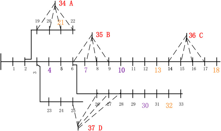
FIGURE 1. Modified IEEE33 node power distribution system.

The newly added power supply substations A, B, C and D respectively correspond to nodes 34, 35, 36 and 37 in the above figure, and the load reference values of the substations are 50, 90, 120, and 200 kVA respectively. The solid line in the figure represents the existing line, and the dotted line represents the line corridor to be built in each new station area; Nodes 4, 7, 10 and 30 are the nodes to be selected for wind turbine access; Nodes 13, 18, 21 and 32 are the nodes to be selected for the access of the photovoltaic unit; Nodes 4, 8, 24, and 32 are demand-side response control nodes; The voltage class of the system is 12.66 kV, the reference power is 100 MV A, the annual average growth rate of the system load is 10%, and all interconnection switches are turned off. The relevant reference prices involved are shown in Table 1 and Table 2.

TABLE 1

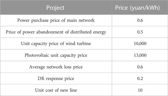
TABLE 1. Relevant reference prices.

TABLE 2

TABLE 2. Length of lines to be built.

5.2 Simulation results and analysis of an example

5.2.1 Correlation processing and uncertainty analysis of random variables

The actual data of a region is taken as the historical data of photovoltaic, wind power and load of the system, and the rank correlation coefficient matrix representing the relationship among the wind speed, light intensity and load of the region is obtained by the above method as follows:

${\mathbf{C}}_W=\left[\begin{array}{ccc}1& -0.1261& -0.0548\\ -0.1261& 1& 0.1730\\ -0.0548& 0.1730& 1\end{array}\right](38)$

At the same time, through independent transformation of the original data, the correlation among the random variables of load, wind power and photovoltaic power generation is eliminated to form mutually independent input random variables, and the per-unit value change curves of the average time sequence output of wind power, average time sequence output of photovoltaic power and load time sequence of the system are obtained by statistics, as shown in Figures 2–4.

FIGURE 2

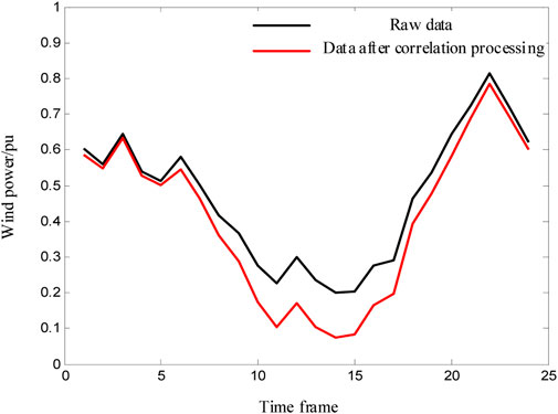
FIGURE 2. Wind power sequence output model.

FIGURE 3

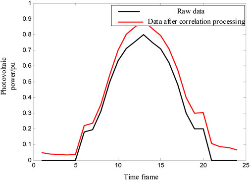
FIGURE 3. Photovoltaic time sequence output model.

FIGURE 4

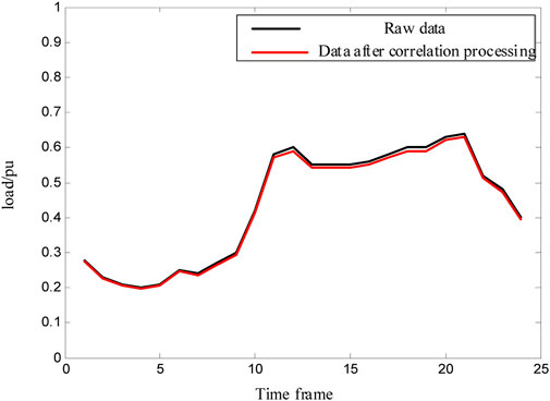
FIGURE 4. Load timing model.

From Figures 2–4, it can be found that after the independent transformation of random variables, the average output percentage of wind power time series decreases significantly on the whole, the photovoltaic power increases significantly on the whole, and the load decreases slightly, while the time series change trend of each random variable remains unchanged on the whole. The main reason for this phenomenon is that there is a certain negative correlation between wind power and PV, wind power and load, and a certain positive correlation between PV and load. In the example of this paper, the wind power output is affected by the superposition and weakening of the negative correlation of PV and load at the same time, and the influence of the positive correlation of load on the output of PV units is more obvious than that of the negative correlation of wind power, while the influence of the positive correlation of PV on the load is relatively smaller than that of the negative correlations of wind power. The average time-sequence output percentage of wind power decreases as a whole, the overall photovoltaic power increases significantly, and the load decreases slightly.

Assume that the annual average load growth rate of the system is $\delta =0.1$, and the time series fluctuation ranges of photovoltaic output, wind power output and load are ${\stackrel{\sim }{\lambda }}_h^{\mathrm{P}}=0.04,\hspace{1em}{\stackrel{\sim }{\lambda }}_h^{\mathrm{P}}=0.02,\hspace{1em}{\stackrel{\sim }{\lambda }}_h^{\mathrm{L}}=0.03$. At the same time, let the conservative index of the uncertainty set is $\mathrm{\Gamma }=2$. Taking the data of load, wind power and photovoltaic power as samples, the uncertainties in the time series variations of wind power, photovoltaic power, and load, post-correlation processing, are depicted as undistributed bounded intervals in Table 3.

TABLE 3

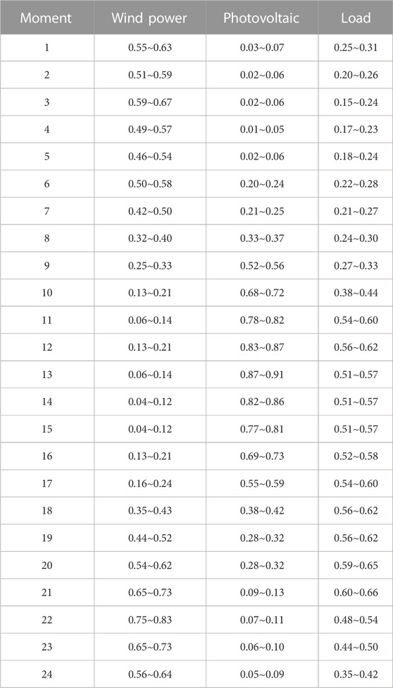
TABLE 3. Time series of random variables without distribution and bounded interval.

5.2.2 Comparison and examination of planning outcomes across various scenarios

In order to verify the effectiveness of this study, for the example in this paper, planning decisions are made in three scenarios:

Scenario 1: a two-stage robust programming model with demand-side response is established and solved considering the correlation among wind energy, solar power and load.

Scenario 2: a two-stage robust programming model with demand-side response is established and solved without considering the correlation among wind energy, solar power and load.

Scenario 3: Considering the influence of correlation in wind energy, photovoltaic power and load, the traditional robust programming model considering demand side response is established and solved.

In the Matlab environment, The Benders method is applied to solve the planning model under various scenarios, and the resulting planning scheme outcomes are presented in Table 4.

TABLE 4

TABLE 4. Planning results under scenario 1.

5.3 Scenario 1 simulation results and analysis

Table 4 displays the best planning strategy for scenario 1.

The costs for the best planning strategy in Scenario 1 are displayed in Table 5.

TABLE 5

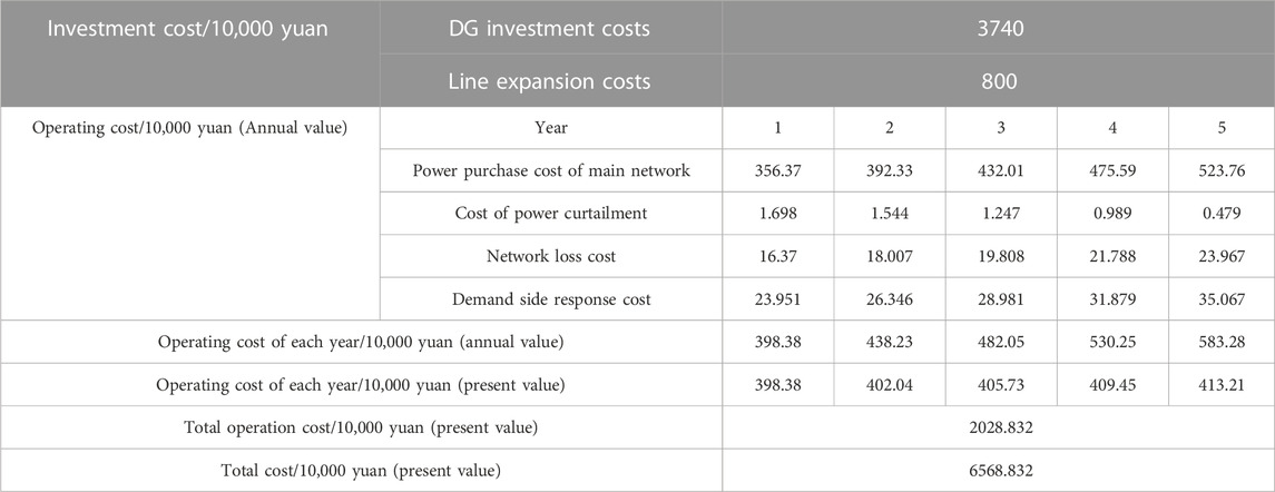
TABLE 5. The cost of the optimal planning scheme in scenario 1.

The table above illustrates that the installed capacity of PV units surpasses that of wind turbines. This is attributed to the inherent anti-peak regulation characteristics of wind power. Overinvesting in wind power can lead to significant curtailment of wind energy during nighttime when demand is low. In contrast, PV output is primarily concentrated during the daytime, which aligns well with higher load demands, allowing for efficient absorption. At the same time, it can be found that the power purchase cost (annual value) of the main grid of the system increases with the increase of load, while the cost of power curtailment decreases with the increase of load. This is because the increased load of the system is borne by two parts: one part is borne by distributed generation, and the increased load at night absorbs part of the curtailment, resulting in the reduction of the cost of power curtailment; The remaining part is borne by the main network, and the increase of electricity purchased by the main network leads to the increase of its cost.

The timing uncertainty interval values for the system random variables in Scenario 1 are presented in Table 6.

TABLE 6

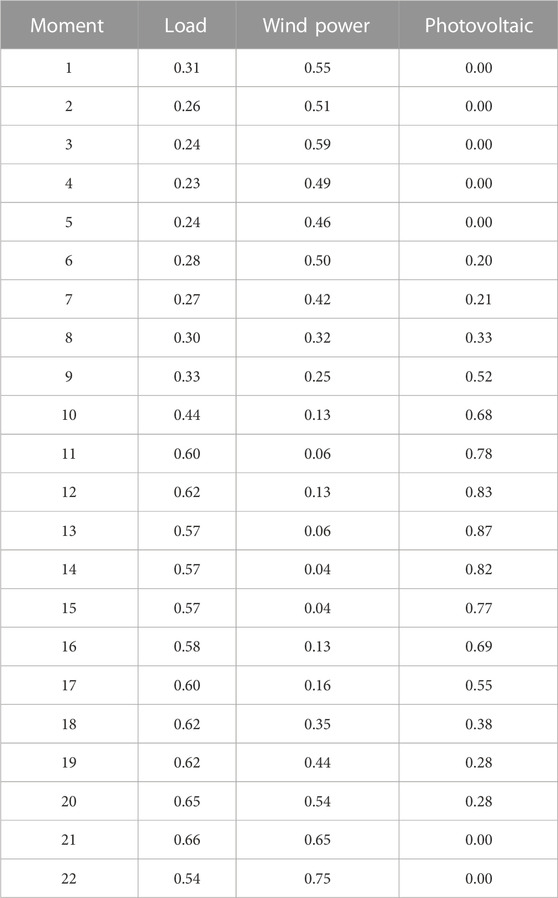
TABLE 6. Values of uncertainty interval of random variables in scenario 1.

From the above table, it can be found that the worst case of the system corresponding to each moment is that the load is taken to the upper bound of the uncertainty interval, the wind and solar energy output are set to the lower bound of the uncertainty interval. Therefore, it can be found that the best planning strategy of the system is formulated under the scenario that the system load reaches the maximum and the wind energy and solar power output reaches the minimum. This is mainly because after the second-order cone transformation, the nonlinear terms of the objective function in this planning model are transformed into the form of second-order cone. According to the fundamental concept of second-order cone optimization, the optimal solution of natural decision-making must be located on the boundary.

The optimal demand-side response strategy in the first year under the optimal planning scheme in Scenario 1 [see Supplementary Material (Appendix) for the remaining four years].

From Table 7, it can be seen that in the example of this paper, the response electric quantity of the demand side of the system is 0 at time 1, 3, 6 and 7, and the response electric quantity of the demand side is very small at time 2, 4, 5, 8 and 9, while obvious load shedding occurs at time 10 to time 24. This is because the wind and solar power generation at a specific time 1, 3, 6 and 7 can fully meet the load demand of the system, and the cost of power curtailment is generated, so there is no need to adjust the demand side response. Although the wind power and PV output of systems 2, 4, 5, 8 and 9 can meet most of the load demand of the system, a portion of the load still needs to be acquired from the higher-tier power grid, and the amount of electricity that can be regulated by demand-side response is very small, so the amount of load shedding is almost negligible. However, from time 10 to time 24, the load of the system greatly exceeds the output of the distributed generation, and there is a large load space for demand-side response regulation, resulting in large load shedding during demand-side response regulation.

TABLE 7

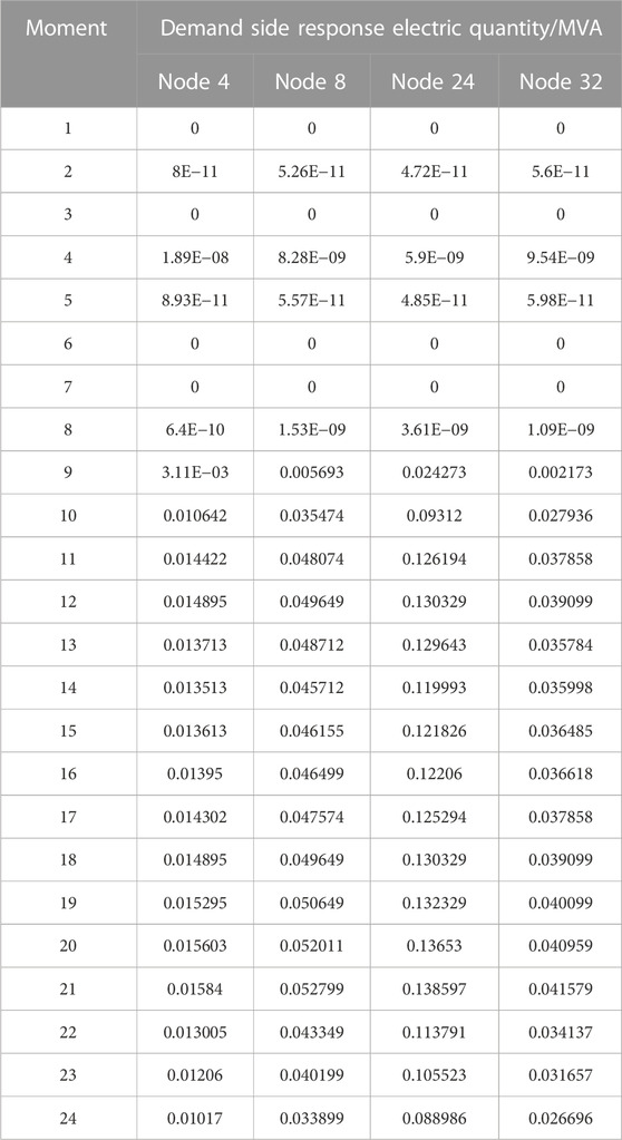
TABLE 7. Optimal demand-side response control strategy in the first year of scenario 1.

At the same time, it can be found from the above table that the general strategy of demand-side response regulation at time 12, 13, 14 and 15 is similar, and time 11 is similar to time 17 and time 18. This is because the load change between time 12 and time 18 is very small, but the decrease (increase) of wind power output is just offset by the increase (decrease) of PV power output between times with similar regulation strategies, which leads to similar demand-side response strategies at different times.

5.4 Scenario 2 simulation results and analysis

To better analyze the correlation’s impact on the simulation planning results in this paper’s example, the optimal planning scheme from scenario 1 is applied to simulate the operations in scenario 2. The resulting system operation costs for the five-year planning period are detailed in Table 8.

TABLE 8

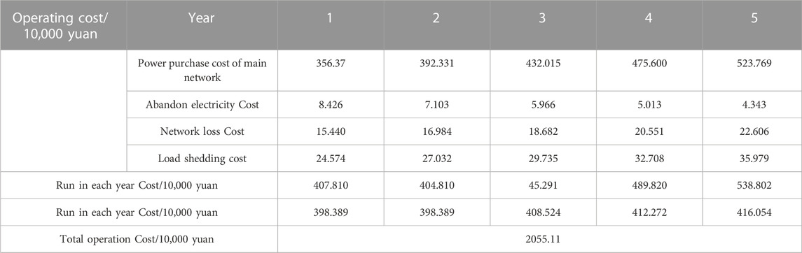
TABLE 8. The operational expenditure for the optimal planning strategy in Scenario 1 under Scenario 2.

It can be seen from the above table that, compared with the operation cost of the optimal planning scheme under scenario 1, in scenario 2, under the same investment conditions, the yearly costs for power procurement, network losses, and load shedding of the main grid have little change, while the power curtailment cost has been significantly increased, and the total cost has also been significantly increased. The reason is that in the example of this paper, the uncertainty interval characterization in scenario 1 is based on the data after correlation processing, while the uncertainty interval characterization in scenario 2 is based on the original data (see Table 5 for details). Compared with scenario 1, the lower boundary of the uncertainty range for wind power is enhanced, whereas for photovoltaic power, it is diminished. The maximum threshold of the uncertainty interval of the load has been slightly raised. Therefore, in the daytime, the reduction of the photovoltaic system’s output unit suppresses the increment of the output of the wind turbine unit, so the slightly increased system load leads to a slight increase in the cost of purchasing electricity, network loss and load shedding in the main network of the system, while the slightly increased system load at night is not enough to absorb the significant increase in the output of wind turbine unit, resulting in a significant increase in system power curtailment cost. To sum up, in the example of this paper, the uncertainty boundary depicted in scenario 2 is worse than that in scenario 1, so the planning strategy obtained by the same planning method in scenario 2 should be more conservative than that in scenario 1. The best planning strategy in Scenario 2 verifies the above conclusion.

The best planning strategy in Scenario 2 is presented in Table 9.

TABLE 9

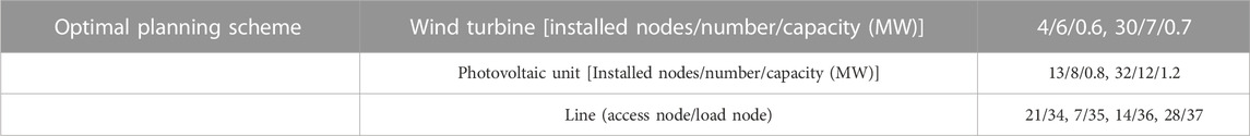
TABLE 9. Planning results under scenario 2.

The expenses associated with the optimal planning strategy in Scenario 2 are displayed in Table 10.

TABLE 10

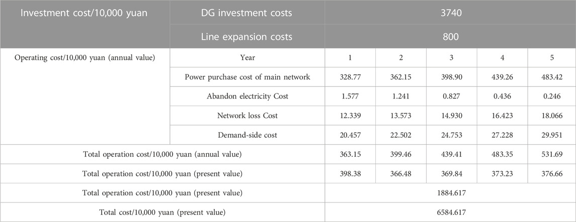
TABLE 10. Cost of optimal planning scheme in scenario 2.

From the table above, it is evident that the capacity is approaching the uncertain boundary of unfavorable natural decision variables compared to scenario 1, and the artificial decision is to deal with the more adverse impact of the system by increasing investment and construction (reducing wind power installed capacity and increasing photovoltaic installed capacity). By comparing with the simulation results under scenario 1, it is found that the total investment cost of the planning scheme without considering correlation is larger than that of the planning scheme with considering correlation, and the investment planning and construction are more conservative.

5.5 Simulation results and analysis of scenario 3

The most effective planning strategy in Scenario 3 is shown in Table 11.

TABLE 11

TABLE 11. Planning results under scenario 3.

The costs in Scenario 2 under the optimal planning scheme are presented in Table 12.

TABLE 12

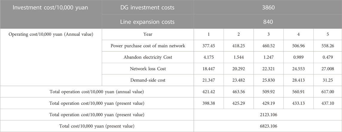
TABLE 12. Cost of optimal planning scheme under scenario 3.

From the above table, it can be seen that compared with scenario 1, the planning results under scenario 3 have increased significantly in terms of both investment cost and operation cost. The main reason for this phenomenon is that the traditional robust optimization model requires all variables to make decisions after the uncertainty is known, allowing nature (uncertain decision variables) to make decisions first, and the artificial system observes the strategies of nature and takes corresponding measures to suppress their adverse effects on the system, so the artificial decision-making is too general. As a result, the planning results are often too conservative.

To sum up, the proposed two-phase robust programming framework, accounting for correlation, considers the impact of random variable correlation on planning outcomes. At the same time, the artificial decision-making is further refined, and it is divided into two stages to resolve the harm brought by the uncertainty of nature. Compared with the traditional robust planning model without considering the influence of correlation, its planning method is finer and the planning result is more economical.

6 Conclusion

In this chapter, the paper introduces a dynamic robust planning method for smart grid systems that considers correlation. Firstly, the Spearman rank correlation coefficient measures the association between different variables. This, combined with the rank correlation matrix characteristics, is utilized in the analysis. Cholesky decomposition and independent transformation are employed to convert correlated random variables into independent ones, and subsequently, the polyhedral uncertainty set is employed to represent the uncertainty. The uncertainties of wind power, PV power and load are represented by bounded intervals without distribution respectively. Finally, combined with the idea of two-stage dynamic robustness, the active distribution network planning problem is described as a game relationship between uncertain decisions controlled by nature and artificial decisions controlled by investors, and a two-stage robust planning model is developed for a dynamic distribution system, taking into account correlation. The results based on standard examples demonstrate the following key findings:

(1) This paper utilizes the Spearman rank correlation coefficient to assess the correlation between wind power, photovoltaic power, and load. It combines this with the properties of the rank correlation matrix, employing methods such as Cholesky decomposition and related independent transformation techniques. These steps effectively convert correlated random variables into independent ones, thereby providing robust data support for distribution network planning. Consequently, this leads to a significant enhancement in the reliability of the distribution network planning results.

(2) The paper adopts the approach of representing uncertainties in wind power, photovoltaic power, and load using the polyhedron uncertainty set representation method. This method employs undistributed bounded intervals to encapsulate the range of potential uncertainties. Additionally, the paper employs the concept of two-stage robust programming to thoroughly integrate the specific circumstances of distribution network planning projects. This enables an accurate simulation of the active distribution network system’s operation, especially at uncertain boundaries. As a result, the reliability and economic efficiency of the active distribution network planning results experience a notable improvement.

Data availability statement

The original contributions presented in the study are included in the article/Supplementary Material, further inquiries can be directed to the corresponding author.

Author contributions

JL: Writing–original draft, Writing–review and editing. BZ: Writing–review and editing. WY: Writing–review and editing. WZ: Writing–review and editing. RC: Writing–original draft. MO: Writing–original draft. TW: Writing–review and editing. TM: Writing–review and editing.

Funding

The author(s) declare financial support was received for the research, authorship, and/or publication of this article. This paper was supported by the Science and Technology Project of Shenzhen Power Supply Corporation, grant number SZKJXM20220036/09000020220301030901283.

Conflict of interest

Authors JL, RC, and MO were employed by Shenzhen Power Supply Company, China Southern Power Grid. Authors BZ, WY, WZ, TW, and TM were employed by China Southern Power Grid.

Publisher’s note

All claims expressed in this article are solely those of the authors and do not necessarily represent those of their affiliated organizations, or those of the publisher, the editors and the reviewers. Any product that may be evaluated in this article, or claim that may be made by its manufacturer, is not guaranteed or endorsed by the publisher.

Supplementary material

The Supplementary Material for this article can be found online at: https://www.frontiersin.org/articles/10.3389/fenrg.2023.1338136/full#supplementary-material

References

Chen, J., Qi, B., Rong, Z., Peng, K., Zhao, Y., and Zhang, X. (2021). Multi-energy coordinated microgrid scheduling with integrated demand response for flexibility improvement. Energy 217, 119387. doi:10.1016/j.energy.2020.119387

CrossRef Full Text | Google Scholar

Chen, R., He, Y., and Chen, F. (2018). Long-term daily load forecasting of electric vehicles based on system dynamics and Monte Carlo simulation. Electr. Power. doi:10.11930/j.issn.1004-9649.201711126

CrossRef Full Text | Google Scholar

Fang, P., Fu, W., Wang, K., Xiong, D., and Zhang, K. (2022). A compositive architecture coupling outlier correction, EWT, nonlinear Volterra multi-model fusion with multi-objective optimization for short-term wind speed forecasting. Appl. Energy 307, 118191. doi:10.1016/J.APENERGY.2021.118191

CrossRef Full Text | Google Scholar

Fu, W., Jiang, X., Li, B., Tan, C., Chen, B., and Chen, X. (2023). Rolling bearing fault diagnosis based on 2D time-frequency images and data augmentation technique. Meas. Sci. Technol. 34, 045005. doi:10.1088/1361-6501/ACABDB

CrossRef Full Text | Google Scholar

Gao, Q., Liu, C., and Jin, D. (2021). Optimizing the configuration of comprehensive energy systems in parks considering comprehensive demand response. High. Volt. Appar. doi:10.13296/j.1001-1609.hva.2021.08.022

CrossRef Full Text | Google Scholar

Li, Q., Wang, L., and Zhang, Y. (2020a). Review of coupling models and dynamic optimization methods for multi energy flow in energy internet. Power Syst. Prot. Control. doi:10.19783/j.cnki.pspc.191309

CrossRef Full Text | Google Scholar

Li, Z., Wan, J., Wang, P., Weng, H., and Li, Z. (2021a). A novel fault section locating method based on distance matching degree in distribution network. Prot. Control Mod. Power Syst. 6, 20. doi:10.1186/S41601-021-00194-Y

CrossRef Full Text | Google Scholar

Li, Z., Wu, L., Xu, Y., Wang, L., and Yang, N. (2023a). Distributed tri-layer risk-averse stochastic game approach for energy trading among multi-energy microgrids. Appl. Energy 331, 120282. doi:10.1016/J.APENERGY.2022.120282

CrossRef Full Text | Google Scholar

Li, Z., Xu, Y., Fang, S., Zheng, X., and Feng, X. (2020b). Robust coordination of a hybrid AC/DC multi-energy ship microgrid with flexible voyage and thermal loads. IEEE Trans. Smart Grid 11, 2782–2793. doi:10.1109/TSG.2020.2964831

CrossRef Full Text | Google Scholar

Li, Z., Xu, Y., Wang, P., and Xiao, G. (2023b). Restoration of multi energy distribution systems with joint district network recon figuration by a distributed stochastic programming approach. IEEE Trans. Smart Grid, 1. doi:10.1109/TSG.2023.3317780

CrossRef Full Text | Google Scholar

Li, Z., Yu, C., Abu-Siada, A., Li, H., Li, Z., Zhang, T., et al. (2021b). An online correction system for electronic voltage transformers. Int. J. Electr. Power Energy Syst. 126, 106611. doi:10.1016/j.ijepes.2020.106611

CrossRef Full Text | Google Scholar

Liao, S., Xu, J., Sun, Y., Bao, Y., and Tang, B. (2018). Control of energy-intensive load for power smoothing in wind power plants. IEEE Trans. Power Syst. 33, 6142–6154. doi:10.1109/tpwrs.2018.2834940

CrossRef Full Text | Google Scholar

Liu, B., Qiu, X., and Han, X. (2016). Research on hierarchical distribution control mode switching of active distribution network. High. Volt. Electr. Appar. doi:10.13296/j.1001-1609.hva.2016.07.01

CrossRef Full Text | Google Scholar

Luo, Y., Shao, Z., and Zhang, L. (2018). Robust economic dispatch and reserve configuration considering wind power uncertainty and gas network operation constraints. J. Electr. Technol. doi:10.19595/j.cnki.1000-6753.tces.170523

CrossRef Full Text | Google Scholar

Peng, X., Lin, L., and Liu, Y. (2015). Optimal configuration of distributed generation based on crisscross-Latin hypercube sampling Monte Carlo simulation metho. Chin. J. Electr. Eng. doi:10.13334/j.0258-8013.pcsee.2015.16.010

CrossRef Full Text | Google Scholar

Shen, X., Ouyang, T., Yang, N., and Zhuang, J. (2021). Sample-based neural approximation approach for probabilistic constrained programs. IEEE Trans. neural Netw. Learn. Syst. 34, 1058–1065. doi:10.1109/TNNLS.2021.3102323

CrossRef Full Text | Google Scholar

Su, L., Li, Z., and Zhang, Z. (2021). Research on coordinated operation strategy of integrated energy microgrid cluster based on chance constrained programming. Power Syst. Prot. Control. doi:10.19783/j.cnki.pspc.200789

CrossRef Full Text | Google Scholar

Sui, Q., Lin, X., and Tong, N. (2020). Economic dispatch of active distribution network based on improved two-stage robust optimization. Chin. J. Electr. Eng. CNKI: SUN: ZGDC.0.2020-07-013. doi:10.13334/j.0258-8013.pcsee.182259

CrossRef Full Text | Google Scholar

Tan, X., Wang, Z., and Li, Q. (2019). Substation capacity and DG confidence capacity probability planning. Power Syst. Technol. doi:10.13335/j.1000-3673.pst.2018.2776

CrossRef Full Text | Google Scholar

Tan, X., Wang, Z., and Shu, D. (2020). Probabilistic planning of the number of substations and feeder lines considering distributed generation. Power Syst. Autom. doi:10.7500/AEPS20200218004

CrossRef Full Text | Google Scholar

Tao, Q., Li, C., and Mu, Y. (2017). Probabilistic capacity planning method for battery energy storage system in isolated microgrid considering demand-side response capability. Proc. CSU-EPSA. doi:10.3969/j.issn.1003-8930.2017.01.007

CrossRef Full Text | Google Scholar

Wang, C., Chu, S., Ying, Y., Wang, A., Chen, R., Xu, H., et al. (2023). Underfrequency load shedding scheme for islanded microgrids considering objective and subjective weight of loads. IEEE Trans. Smart Grid 14, 899–913. doi:10.1109/TSG.2022.3203172

CrossRef Full Text | Google Scholar

Wang, Z., Lou, S., and Fan, Z. (2019). Congestion scheduling optimization for power systems with large-scale wind power based on chance constrained programming. Power Syst. Autom. doi:10.7500/AEPS20181219003

CrossRef Full Text | Google Scholar

Wang, Z., Zhang, Z., Li, Y., Wang, T., and Liao, X. (2021). Coordinated scheduling method of integrated energy supply side under multi-energy complementary environment. Energy Environ. Prot. doi:10.19389/j.cnki.1003-0506.2021.12.030

CrossRef Full Text | Google Scholar

Xiao, K., Qiu, W., and Tao, Y. (2021). Fuzzy chance constraint method for optimal scheduling of energy storage emergency vehicles. High. Volt. Electr. Appliances. doi:10.13296/j.1001-1609.hva.2021.02.017

CrossRef Full Text | Google Scholar

Xiao, L., Xie, Y., and Hu, H. (2022). Bi-level optimal scheduling strategy for charging and discharging of electric vehicles based on V2G. High-Voltage Electr. Appliances. doi:10.13296/j.1001-1609.hva.2022.05.022

CrossRef Full Text | Google Scholar

Xu, P., Fu, W., Lu, Q., Zhang, S., Wang, R., and Meng, J. (2023). Stability analysis of hydro-turbine governing system with sloping ceiling tailrace tunnel and upstream surge tank considering nonlinear hydro-turbine characteristics. Renew. Energy 210, 556–574. doi:10.1016/J.RENENE.2023.04.028

CrossRef Full Text | Google Scholar

Yang, N., Dong, Z., Wu, L., Zhang, L., Shen, X., Chen, D., et al. (2022b). A comprehensive review of security-constrained unit commitment. J. Mod. Power Syst. Clean Energy 10, 562–576. doi:10.35833/MPCE.2021.000255

CrossRef Full Text | Google Scholar

Yang, N., Qin, T., Wu, L., Huang, Y., Huang, Y., Xing, C., et al. (2022a). A multi-agent game based joint planning approach for electricity-gas integrated energy systems considering wind power uncertainty. Electr. Power Syst. Res. Mar 204, 107673. doi:10.1016/j.epsr.2021.107673

CrossRef Full Text | Google Scholar

Yang, N., Ye, D., Zhou, Z., Jiazhan, C., Daojun, C., and Xiaoming, W. (2018). Research on modelling and solution of stochastic SCUC under AC power flow constraints. IET Generation, Transm. Distribution 12 (15), 3618–3625. doi:10.1049/iet-gtd.2017.1845

CrossRef Full Text | Google Scholar

Yu, G., Liu, C., Tang, B., Chen, R., Lu, L., Cui, C., et al. (2022). Short term wind power prediction for regional wind farms based on spatial-temporal characteristic distribution. Renew. Energy 199, 599–612. doi:10.1016/J.RENENE.2022.08.142

CrossRef Full Text | Google Scholar

Yu, Z., Qiao, Z., and Lei, W. (2023). Optimal operation of regional microgrids with renewable and energy storage: solution robustness and nonanticipativity against uncertainties. IEEE Trans. Smart Grid. doi:10.1109/TSG.2022.3185231

CrossRef Full Text | Google Scholar

Zeng, M., Zhang, P., and Wang, L. (2015). Power generation investment evaluation model based on Monte Carlo simulation under uncertain conditions. Power Syst. Autom. doi:10.7500/AEPS20140625014

CrossRef Full Text | Google Scholar

Zhang, Y., Ai, X., Fang, J., and He, H. (2019). Data-adaptive robust optimization method for the economic dispatch of active distribution networks. IEEE Trans. Smart Grid 10, 3791–3800. doi:10.1109/TSG.2018.2834952

CrossRef Full Text | Google Scholar

Zhang, Y., Wei, L., Fu, W., Chen, X., and Hu, S. (2023). Secondary frequency control strategy considering DoS attacks for MTDC system. Electr. Power Syst. Res. 214, 108888. doi:10.1016/J.EPSR.2022.108888

CrossRef Full Text | Google Scholar

Zhang, Y., Xie, X., Fu, W., Chen, X., Hu, S., Zhang, L., et al. (2022). An optimal combining attack strategy against economic dispatch of integrated energy system. IEEE Trans. Circuits Syst. II Express Briefs 70, 246–250. doi:10.1109/tcsii.2022.3196931

CrossRef Full Text | Google Scholar

Zheng, G., Li, H., Zhao, B., Wu, B., and Tang, W. (2018). Comprehensive optimization of electrical/thermal energy storage equipments for integrated energy system near user side based on energy supply and demand balance. Dianli Xit. Baohu yu Kongzhi/Power Syst. Prot. Control 170. doi:10.7667/PSPC171221

CrossRef Full Text | Google Scholar

Zhou, C., Jia, H., and Jin, X. (2023). Coordinated optimization of intelligent building and community integrated energy system based on chance constrained programming. Power Syst. Autom. doi:10.7500/AEPS20220507007

CrossRef Full Text | Google Scholar

Zhou, W., and Zhao, S. (2013). Quantitative analysis of traveler route choice behavior based on Mixed Logit model. J. Jilin Univ. Technol. Ed. 43. doi:10.13229/j.cnki.jdxbgxb2013.02.040

CrossRef Full Text | Google Scholar

Zhu, B., Liu, Y., Zhi, S., Wang, K., and Liu, J. (2023). A family of bipolar high step-up zeta–buck–boost converter based on “coat circuit”. IEEE Trans. Power Electron. 38, 3328–3339. doi:10.1109/TPEL.2022.3221781

CrossRef Full Text | Google Scholar