 Jiawen Li
 Minghao Liu2*
- 1Hangzhou Digital Energy and Low Carbon Technology Co., Ltd., Hangzhou, China
- 2Department of Mathematics and Physics, North China Electric Power University, Baoding, China
- 3Department of Economics and Management, North China Electric Power University, Baoding, China
Wind power generation has aroused widespread concern worldwide. Accurate prediction of wind speed is very important for the safe and economic operation of the power grid. This paper presents a short-term wind speed prediction model which includes data decomposition, deep learning, intelligent algorithm optimization, and error correction modules. First, the robust local mean decomposition (RLMD) is applied to the original wind speed data to reduce the non-stationarity of the data. Then, the salp swarm algorithm (SSA) is used to determine the optimal parameter combination of the bidirectional gated recurrent unit (BiGRU) to ensure prediction quality. In order to eliminate the predictable components of the error further, a correction module based on the improved salp swarm algorithm (ISSA) and deep extreme learning machine (DELM) is constructed. The exploration and exploitation capability of the original SSA is enhanced by introducing a crazy operator and dynamic learning strategy, and the input weights and thresholds in the DELM are optimized by the ISSA to improve the generalization ability of the model. The actual data of wind farms are used to verify the advancement of the proposed model. Compared with other models, the results show that the proposed model has the best prediction performance. As a powerful tool, the developed forecasting system is expected to be further used in the energy system.
1 Introduction
Efficient use of energy promotes rapid development of society and economy. In recent years, the human society’s demand for energy has been increasing, and the excessive consumption of fossil fuels will not only cause serious environmental pollution but also lead to the energy crisis. In order to alleviate the contradiction between energy supply and demand, wind energy, as a renewable energy with abundant resources and low cost, has been widely concerned by scientists all over the world (Liu et al., 2023). The inherent intermittency and volatility of wind power can have a negative impact on power dispatching and power quality. Wind speed is a key factor affecting wind power output. Improving wind speed prediction accuracy is an effective way to improve the operation economy of the power grid and ensure the safe and stable operation of the power grid (Ying et al., 2023).
According to the existing forecasting technology, wind speed forecasting methods can be divided into physical models, statistical models, and artificial intelligence models. The physical model generally uses various meteorological parameters to predict wind speed on the basis of a large number of calculations. In the calculation process, a large number of terrain conditions are mixed, and the physical boundary conditions around the wind turbine need to be considered. The equation-solving process is time-consuming, and the meteorological data are difficult to obtain. Numerical weather prediction (NWP) is a typical physical model (Hoolohan et al., 2018; Ahmadpour and Farkoush, 2020). Statistical models are based on historical data, and Karaku et al. (2017) used the autoregressive (AR) model to verify the short-term prediction effect. In addition, autoregressive moving average (ARMA) (Erdem and Shi, 2011), autoregressive integrated moving average (ARIMA) (Yunus et al., 2016; Sabat et al., 2023), autoregressive fractionally integrated moving average (ARFIMA) (Yuan et al., 2017), and other models have been developed to extract the implied information in historical wind speed series, and the results show that the statistical model has a good analytical performance in analyzing linear relationships. However, it is difficult to deal with the nonlinear relationship between the data.
To further explain the nonlinear relationship between the data, the researchers proposed a series of artificial intelligence models, such as the artificial neural network (Ates, 2023) and the least square support vector machine (LSSVM) (Zhao et al., 2022). They have been developed rapidly because of their good adaptability to various non-stationary data. Wang C. H. et al. (2023a) used the backpropagation (BP) neural network to predict wind power, and the experimental results confirmed the outstanding advantages of complex neurons in adaptive ability and nonlinear expression. Liu et al. (2020) used a support vector machine (SVM) to predict wind speed data, and the experimental results verified the feasibility of the SVM for regression prediction. Tian et al. (2021) used the echo state network (ESN) to reflect the changing law of wind speed correctly. Shang et al. (2022) built the ELMAN model and obtained better prediction results. At the same time, the extreme learning machine (ELM) has the characteristics of few parameters, fast learning speed, and strong generalization ability and has been applied in the field of prediction (Adnan et al., 2021; Syama et al., 2023). With the development of computer hardware, many deep learning networks have been developed for wind speed prediction. López and Arboleya, (2022) used the long short-term memory (LSTM) model to improve short-term wind speed prediction performance. Tian and Chen, (2021b) proposed a reinforced LSTM model, and the result showed the effectiveness of the improved model structure. Han et al. (2023) introduced the convolutional neural network (CNN) to extract potential wind speed information and adopted LSTM as the prediction network, and the results verified that the proposed model has reliable prediction performance. Niu et al. (2020) embedded the attention mechanism into the gated recurrent unit (GRU) model to improve the model’s peak prediction ability. Liang et al. (2023) proposed a deep space–time residual network (DST-ResNet) for wind speed prediction. Lin et al. (2023) used the shifted window stationary attention (SWSA) transformer to fully extract complex wind speed characteristics, and the results showed the reliability of the prediction model. Bommidi et al. (2023) used the attentional temporal convolutional network (ATCN) based on the attention mechanism to extract important features of wind speed, and Bi-LSTM was used to output prediction results.
The original wind speed data usually have strong non-stationarity, and the nonlinear characteristics of the data can be reduced by using signal decomposition technology to improve the prediction accuracy of the model. So far, various methods including empirical wavelet transform (EWT) (Gao et al., 2021), complete set empirical mode decomposition with adaptive noise (CEEMDAN) (Gao et al., 2020), empirical mode decomposition (EMD) (Jiang et al., 2021), wavelet transform (WT) (Chi and Yang, 2023), ensemble empirical mode decomposition (EEMD) (Tian et al., 2020), and singular spectrum analysis (SSA) (Yan et al., 2020) have been used for wind speed decomposition. Lv et al. (2022) used the variational mode decomposition (VMD) method to decompose historical wind speed data and express the information characteristics of the original signal on different scales. Tian (2021) used adaptive variational mode decomposition to process the data and obtained a reasonable number of decomposition modes. Wang J. Z. et al. (2023b) used ICEEMDAN data denoising technology to build a wind quantile prediction component. Local mean decomposition (LMD) is highly adaptable and provides a good solution for decomposing signal features (Tian, 2020b; Peng et al., 2021). Wang et al. (2022) used robust local mean decomposition (RLMD) as a signal processing tool, and the data simulation confirmed the decomposition ability of RLMD. In addition to the above data preprocessing methods based on time–frequency signal decomposition, many intelligent algorithms are used to optimize the parameters of the prediction model to improve the prediction accuracy. In particular, the prediction effect of deep neural networks will be significantly affected by the inherent structure and parameters (Li et al., 2022). Common optimization algorithms in the field of wind speed prediction include gray wolf optimization (GWO) (Hu et al., 2022), particle swarm optimization (PSO) (Tian and Chen, 2021a; Zhang and Wang, 2022), atom search optimization (ASO) (Fu et al., 2021), and whale optimization algorithm (WOA) (Alhussan et al., 2023). Xiang et al. (2020) used the chicken flock optimization algorithm to jointly optimize the PSR-GRU model and obtained the best prediction network structure. Tuerxun et al. (2022) adopted the improved CONDOR optimization algorithm to optimize the hyperparameters in LSTM, and the experiment achieved satisfactory prediction results. Zhang et al. (2022b) improved the sine–cosine algorithm by adding a uniform initialization and nonlinear strategy to optimize the parameters of the BiLSTM model. Tian (2020a) used the backtracking search algorithm to optimize the LSSVM, which enhanced the prediction effect. An et al. (2022) adopted the improved slime mold algorithm (ISMA) to optimize the weights and thresholds of the deep extreme learning machine (DELM), which improved the prediction accuracy of short-term wind power.
To further improve the forecasting effect, error correction is often used in wind speed forecasting systems. Zhang et al. (2021) used the Markov chain model to process the error sequence and further extract the available information in the sequence. Ding et al. (2022) proposed an error segmentation processing method, and each error was processed by the ARIMA model, which improved the prediction accuracy. Zhang Y G et al. (2022) proposed a decomposition piecewise error correction (DSEC) technique, and experiments verified the effectiveness of the proposed framework. Tang et al. (2021) established an error correction model based on the LSSVM to correct the initial prediction results. Jiao et al. (2023) proposed an error correction technique based on the ELM to reduce the deviation between the predicted wind speed and the actual value. Liu and Chen, (2019) used the outlier robust extreme learning machine (ORELM) to capture the predictable components of the error sequence, and the results show that the model has more robust adaptability. The unextracted rule information in the initial prediction can be mined by error correction to enhance the prediction ability of the model.
Based on the above analysis, this paper proposes a novel hybrid multi-step prediction model, namely, RLMD-O-BiGRU-ISSA-DELM, which consists of four parts: data decomposition, bidirectional deep learning, intelligent algorithm optimization, and error correction. First, the model decomposes the initial wind speed sequence using RLMD to obtain a series of characteristic components. Each component is then trained and predicted by the bidirectional gated recurrent unit (BiGRU) network, and in order to improve the prediction accuracy, the salp swarm algorithm (SSA) is used to optimize BiGRU hyperparameters. On the basis of error analysis, the DELM model is established, and the weights and thresholds of the DELM model are optimized by using the improved SSA, and then the initial prediction results are modified. The effectiveness and superiority of the proposed model are verified through comparative analysis of cases. The main contributions of this paper are as follows:
(1) RLMD technology can solve the end effects and mode mixing problems generated in the decomposition process, effectively explain the volatility and trend of wind speed series, and improve the robustness performance. At the same time, RLMD optimizes the envelope estimation and stopping criteria of the LMD to reduce the non-stationarity and non-linearity of the initial sequence.
(2) Aiming at the low optimization accuracy of the basic SSA in the face of high dimensions, an improved salp swarm algorithm (ISSA) is proposed. The ISSA adopts piecewise mapping to improve the initial individual diversity. We introduce a crazy operator and dynamic learning strategy to increase the population diversity and enhance the exploitation and exploration capability of the algorithm.
(3) Combining the SSA with the deep learning network makes use of algorithm characteristics of few parameters and fast solution. The SSA is used to optimize the number of neurons, learning rate, and batch size in deep neural networks, and the best combination of hyperparameters is found to enhance the quality of prediction.
(4) The DELM model is constructed by generating the error sequence through prelim-nary prediction, and the predictable components in the error sequence are mined. The ISSA is introduced into the optimization process of DELM parameters. The optimal weights and thresholds are found in the global scope, effectively improving the prediction accuracy.
2 Materials and methods
This section introduces the basic methods for the four parts of the proposed model, i.e., RLMD for data decomposition, BiGRU and DELM for prediction, and improvement and application of intelligent algorithms. At the same time, a complete prediction framework is proposed.
2.1 Robust local mean decomposition
The LMD method is an adaptive analysis method for non-stationary signals, which can adaptively decompose the frequency modulation and amplitude modulation signals into a set of product functions, and each product function is the product of the instantaneous envelope signal and the pure frequency modulation signal. For a given signal x(t), the LMD decomposition steps are as follows (Smith, 2005):
(1) According to all local extreme points ni, the mean value mi of all local extreme values and the envelope estimate ai are obtained: the local mean function m11(t) and the envelope function a11(t) are obtained after processing by using the moving average method.
(2) Function h11(t) uses the local mean function to separate the original signal x(t) and demodulate it to function s11(t): repeat the above steps to obtain s12(t) as the s11(t) new function until s1n(t) is a pure frequency modulation function.
(3) Obtain the envelope signal:
(4) Obtain the first PF component:
(5) After separating PF1(t) from x(t) and obtaining u1(t), the above calculation process is repeated with u1(t) as a new original signal. Stop the calculation when uq(t) is obtained as a monotonic function.
(6) The original signal is decomposed into
The LMD method may have the limitations of end effect and mode mixing. In order to alleviate the interference of these two limitations, Liu et al. (2017) proposed RLMD. Signal decomposition using RLMD can better obtain useful modal components that reflect the essential characteristics of signals. The specific improvement process is as follows:
(1) Boundary conditions: The symmetric points at the left and right ends of the signal are determined using the image extension algorithm.
(2) Envelope estimation: According to the statistical theory, an optimal subset size λ∗ is obtained.
where s(k) is the step size between local average signals or local amplitude signals. μs and δs are the mean and standard deviation corresponding to the step s(k) between the smooth local mean mk and the smooth local amplitude ak, respectively. odd(.) is an operation that returns the nearest odd integer greater than or equal to the input. μs and δs can be expressed as follows:
where f(k) represents the probability of each box number obtained by counting the step length set using the histogram box number; Nb represents the number of boxes.
(3) Filter stop criteria: Minimize the following function f(x):
where RMS [z(t)] and EK [z(t)] can be expressed as follows:
where z(t) is zero-base line envelope signal;
2.2 Bidirectional gated recurrent unit
In order to solve the problem of long short-term memory loss in recurrent neural networks, the long short-term memory network (LSTM) and GRU are proposed successively. The GRU simplifies the gating unit in the LSTM logical unit, requires less memory consumption, and can effectively solve the problem of gradient disappearance in the training process of traditional recurrent neural networks. The GRU calculation process for the input is as follows (Cho et al., 2014):
where σ(∙) and tanh (∙) are activation functions; x(t) is the input at time t; ht-1 is the hidden state at time t-1; and the hidden state at the initial time is 0. zt, rt, and nt are the update gate, the reset gate, and the calculated candidate hidden layer, respectively. Wiz, Wir, and Win are the corresponding weight matrices.
The BiGRU network (Li et al., 2022) is composed of two GRU networks in opposite directions. Figure 1 shows the BiGRU network structure composed of GRUs. S0 and S1 represent the initial positions of the two propagation directions, respectively, where Xt-1, Xt, and Xt+1 represent the input that changes over time, and ht-1, ht, and ht+1 represent the hidden state that changes over time. Compared with the GRU network, the nodes of the BiGRU network at every moment contain the information of the entire input sequence, which can better feature the expression of the entire input sequence.
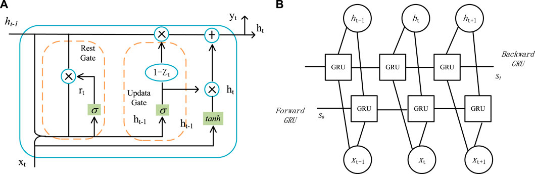
FIGURE 1. Structure of the GRU and BiGRU networks. (A) Structure of the GRU. (B) Structure of the BiGRU network.
2.3 Deep extreme learning machine
The ELM is a single hidden layer feedforward neural network (Huang et al., 2004). In the training process, the input weights and thresholds of the hidden layer are randomly generated, and only the generalized inverse matrix theory can be used to calculate the weights to complete the learning. Therefore, the ELM network has the advantages of fast learning speed and strong generalization ability.
The DELM uses the combination of the extreme learning machine and automatic encoder to form the ELM-AE structure, which is used as the basic unit of unsupervised learning to train and learn input data. It saves the output weight matrix obtained using the least-square method for the stack multi-layer extreme learning machine (ML-ELM). Compared with other neural networks, DELMs can capture the mapping relationship between data more comprehensively and effectively improve the ability to deal with high-dimensional and non-linear data.
Assuming that the DELM has R group training data {(xi,yi)|i = 1,2,⋯,R} and M hidden layers, the first weight matrix β1 of the training data is obtained according to the autoencoder extreme learning machine theory, and then the eigenvector H1 of the hidden layer is obtained. Furthermore, the input layer weight matrix and the hidden layer feature vector of layer M can be obtained. The expression of the DELM mathematical model is as follows (Ding et al., 2015):
where L is the number of hidden layer neurons; Z is the number of derived neurons corresponding to the hidden layer neurons; β is the weight vector between the Kth derived neuron corresponding to the Jth hidden layer neuron and the output layer; g is the K derivative of the neuron activation function of the Jth hidden layer. N is the number of neurons in the input layer; W is the weight vector between the input layer and the Jth hidden layer neurons. b is the bias of the Jth hidden layer node.
2.4 Improved salp swarm algorithm
2.4.1 Salp swarm algorithm
In order to achieve rapid coordinated movement, marine salps usually gather together to form moving salp chains, and a mathematical model is constructed according to the actual movement law of the chain (Mirjalili et al., 2017). The salp population forming the chain is divided into two groups: leaders and followers. The leader is at the front end of the chain, leading the entire population to approach the food source, and the rest of the individuals are followers, guided by the leader to move. Similar to other intelligent algorithms, the location of salps is defined in a J-dimensional search space, assuming that there is a food source defined as F in the search space, which is the moving target of the salp swarm.
In the algorithm iteration process, the food source represents the position of the individual with the best fitness in each generation, and the leader in the population gradually approaches the food source and moves around it. During the movement, the leader’s update position is described as follows:
where xj represents the position of the leader in the jth space, Fj represents the location of the food source in the jth space, and ub and lb represent the upper and lower boundaries of the jth space, respectively. c2 and c3 represent random numbers in the interval [0,1, respectively].
c1 balances the two processes of exploration and exploitation, which is described as follows:
where t represents the current iteration, and max represents the maximum iteration.
In the salp chain structure, each follower moves based on the position of the previous individual, and the update formula of the follower is as follows:
where
By means of the location updating strategy and adjustment of control factor c1, the SSA can gradually find the optimal solution in the search space.
2.4.2 Chaos initialization
The SSA is the same as many swarm intelligence algorithms, which randomly generates the initial position. It is easy to cause the uneven position distribution of salps, resulting in poor diversity. Chaotic mapping has good ergodicity and non-repeatability, so it can be used to replace random population initialization. Piecewise mapping (Zhang et al., 2022a) is a typical representative of chaotic mapping. By initializing the location of the salp population through piecewise mapping, the population can be more evenly distributed in the search space. Its mathematical formula is as follows:
The range of P and x in the piecewise expression is [0,1], and k is the sequence number of the chaos variable.
2.4.3 Crazy operator
The location of the food source represents the optimal direction of population search in the SSA. If the location of the food source appears near the local optimal, the search process of the population is likely to stop, resulting in the decline of intra-group diversity. In the process of the algorithm iteration, the food source constantly changes its location to enhance the diversity of the population. The crazy operator (Wang et al., 2013; Zhang et al., 2020) is introduced into the leader position update formula to generate a certain disturbance to the food source position so as to avoid the algorithm falling into local optimal and enhance the global optimal searchability. The update leader formula is as follows:
where c4 is a random number with uniform distribution in the interval [0,1] and xcraziness is usually a smaller constant, which is set to 0.001 in this paper. P (c4) and sign (c4) are defined as follows:
where Pcr is the crazy operator probability, and the probability of the food source moving during the movement of salps is small in practice. If the crazy operator probability is set to 0.3, the random number c4 will have a high probability, greater than Pcr, and the P(c4) will also be 0.
2.4.4 Dynamic learning strategy
The follower’s position updating process is not affected by any parameters in the process of algorithm iteration, and its moving position is determined by the individual’s own position and the position of the previous individual, which may lead to the phenomenon of salps population blindly following. Weight factors are added to the positions of individuals with inferior fitness to reduce the influence of individuals with poorer positions by introducing a dynamic learning strategy (Jia et al., 2023), and then the weight of individuals with better fitness is increased, enhancing the influence weight of elite individuals. In the process of convergence, elite individuals can better play an assisting role and strengthen the local exploration ability of the algorithm.
where
2.4.5 Implementation flow of the ISSA
In this paper, an improved SSA is obtained by adding chaotic mapping in the initialization stage, perturbating the food source through crazy operators, and introducing the dynamic learning strategy into the position update process of the follower. The improvement measures enhance the diversity of the population, effectively balance the exploration and exploitation ability of the algorithm, and reduce the blindness of followers, so the ISSA has a strong optimization ability. The implementation process of the improved algorithm is defined as follows:
Step 1: Setting algorithm parameters, including the maximum number of iterations, population size, and upper and lower limits of parameters.
Step 2: Initializing the population. The chaotic sequence is generated by piecewise mapping, and then the chaotic sequence is inversely mapped into a search matrix according to the upper and lower boundaries of the search space.
Step 3: The initial fitness value is calculated, and the optimal individual is selected as the food location.
Step 4: Location update. The leader uses the formula disturbed by the crazy algorithm to update the position, and the follower updates the position through the formula adjusted by the dynamic learning strategy.
Step 5: The fitness value of the updated population is calculated, and the food source location is updated.
Step 6: Determining the end condition. When the specified maximum number of iterations is reached, the algorithm terminates and a global optimal solution is obtained. Otherwise, perform steps 4–6.
2.4.6 Assessment for the ISSA
To demonstrate the superiority of the ISSA, it is compared with several common algorithms, such as DE, DA, PFA, ASO, PSO, and SSA. The parameter values of each algorithm are shown in Table 1. For fair evaluation, the search agent and the maximum number of iterations of the algorithms are 30 and 500, respectively, and each algorithm runs independently 30 times on average. A total of 13 test functions (Yao et al., 1999) are used to test the algorithm in 50 dimensions, among which F1–F7 is the unimodal function and F8–F13 is the multi-modal function. A detailed description of the benchmark function is provided in Mirjalili and Applications (2016).
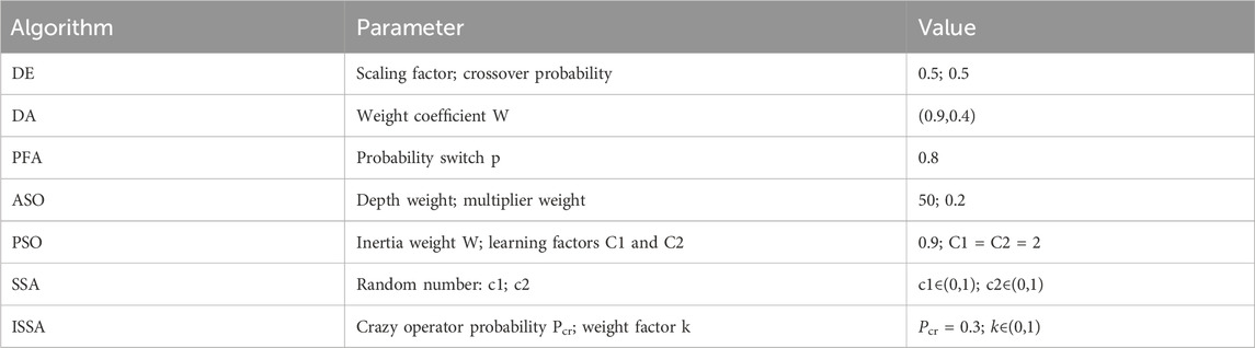
TABLE 1. Basic parameters of the relevant algorithm.
The specific experimental results are summarized in Table 2, where the best experimental results are given in bold. It can be clearly seen from Table 2 that the ISSA shows excellent convergence accuracy and stability in unimodal and multi-modal functions on the whole, which proves that it has good global exploitation and local exploration capabilities. The convergence curves of each algorithm on some of the test functions are shown in Figure 2. It can be seen from the image that the ISSA has the fastest convergence speed and can quickly approximate the global optimal solution. Chaotic mapping makes the population distribution more uniform. Introducing crazy operators and the dynamic learning strategy solves the problem of premature convergence and local optimal of other algorithms, thus improving the convergence speed.
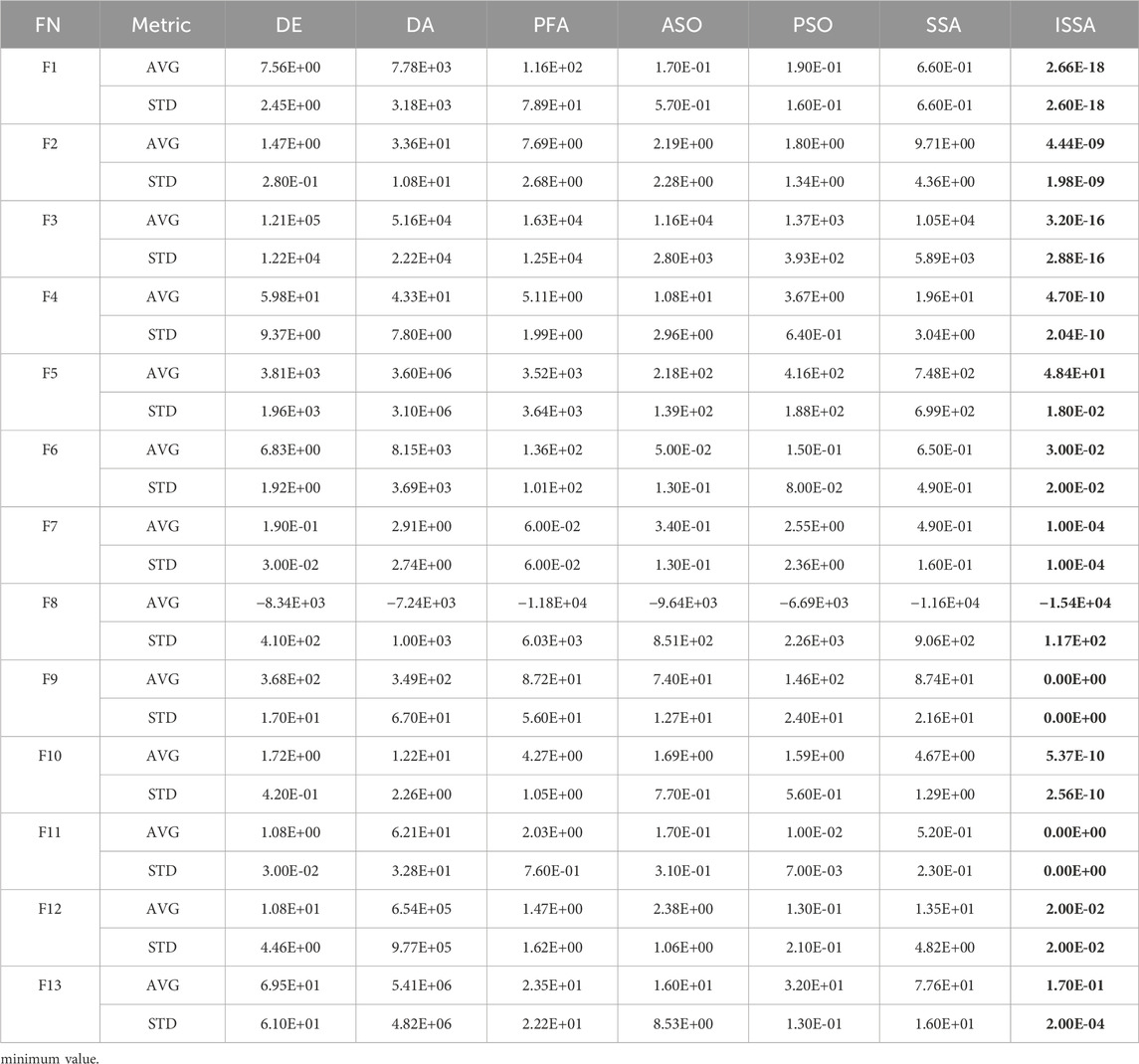
TABLE 2. Performance of the ISSA compared to other algorithms.
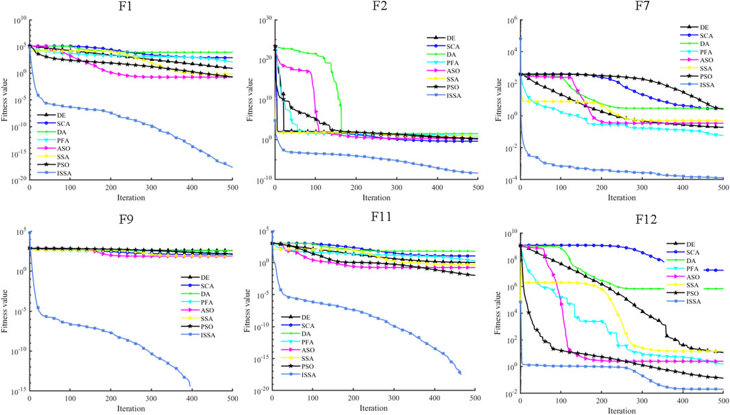
FIGURE 2. Convergence curves of the DE, SCA, DA, PFA, ASO, SSA, PSO, and ISSA tested on various benchmark functions.
2.4.7 Parameter optimization
The learning ability of the deep learning model depends heavily on the parameter settings. The selection of hyperparameters by manual experience cannot meet the needs of different projects and cannot give full play to the learning performance of the model. In general, the parameters that affect the prediction performance of the model include the number of hidden layer neurons, batch size, and learning rate. So the coordinated combination of different parameters can make the model exert maximum performance. In the proposed model of this paper, the SSA is used to optimize the three hyperparameters of the deep learning model, namely, the number of units, batch, and learning rate. The SSA has the advantages of simple structure, few parameters, and convenient operation. Combined with the deep network, the algorithm can ensure convergence accuracy without increasing complexity. However, the SSA has the disadvantages of slow convergence speed and difficult balance between exploration and exploitation ability in the face of multi-dimensional complex problems. To solve the above problems, this paper proposes an improved SSA, which uses piecewise mapping to increase the number of the initial population. Crazy operators are introduced to enhance the global optimal search ability. Meanwhile, the dynamic learning strategy is adopted to update the followers’ movement mode and improve the local exploration ability of the algorithm. The improved SSA is combined with the DELM model to process the error sequence and then revise the initial prediction results.
2.5 Modeling process
The paper proposed a multiple-step wind speed forecasting model based on RLMD, SSA, ISSA, BiGRU, and DELM. The flow chart is shown in Figure 3. The corresponding modeling steps are as follows:
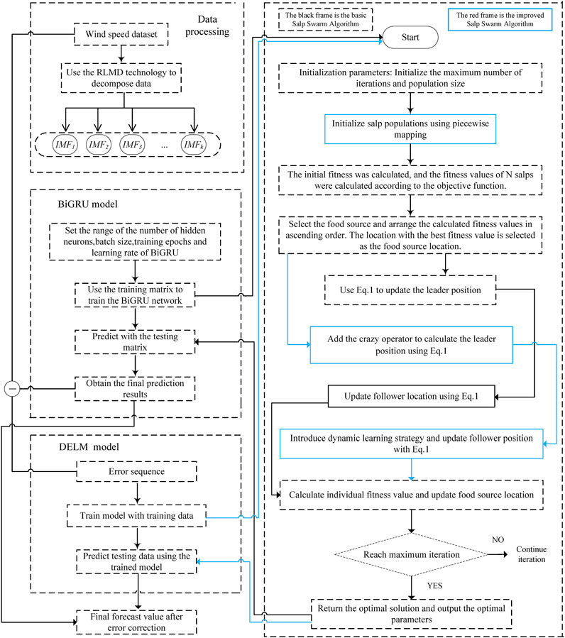
FIGURE 3. Flow chart of the proposed prediction model.
Step 1: Collecting the original wind speed sequence.
Step 2: By processing the original wind speed data using RLMD, multiple IMF components are obtained, and train sets and test sets of components are divided.
Step 3: The SSA is used to optimize the BiGRU parameters.
Step 3.1: Initializing the SSA, including the population size and the maximum number of iterations of the algorithm. The learning rate, the number of hidden layer neurons, and the batch size are taken as the target optimization parameters of the SSA.
Step 3.2: Performing the training process through the training data and taking the mean square error of the predicted value and the true value as the fitness function. The BiGRU parameter is iteratively updated until the maximum number of iterations is reached, and the optimal network structure parameter value is returned.
Step 4: Inputting the test set data into the trained SSA-BiGRU model, and the predicted value of each component is superimposed to obtain the final predicted value.
Step 5: Obtaining the error sequence from the original data and preliminary prediction data.
Step 6: Using the ISSA-DELM model to predict the error sequence.
Step 6.1: Initializing individuals in the salp population using the piecewise mapping strategy. Crazy operators and a dynamic learning strategy are used to enhance the exploitation and exploration ability of the original algorithm, and an improved SSA is obtained.
Step 6.2: The mproved SSA is used to find the optimal combination of weights and thresholds in the DELM, and the trained model is used for error prediction.
Step 7: The prediction results of the final wind speed series are obtained by summarizing the preliminary prediction results and the error series prediction results.
3 Case study
3.1 Data description and decomposition
This paper selects the actual data of a wind farm in central China, which is divided into the wind speed data set of January and the wind speed data set of July. The average sampling period is 10 min, and 144 sample points are collected every day. The total number of data sets is 2,880, with a total of 20 days of data. The first 15 days of data are the training set, and the following 4 days of data are used to train the error model. The prediction performance of all models is evaluated using the data of the 144 sample points of the last day. Figure 4A shows the visualizations of two wind speed time series.
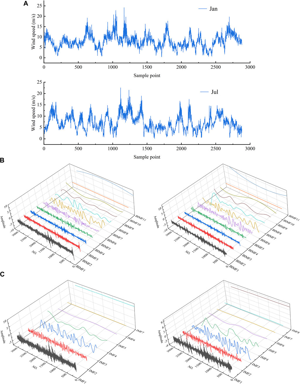
FIGURE 4. (A) Short-term wind speed data sets. (B) EMD results. (C) RLMD results.
Due to the random characteristics of the wind speed series, it is necessary to decompose the wind speed for the sake of improving the overall prediction accuracy. In this paper, EMD and RLMD methods are used to separate and extract multiple frequency components of wind speed data. As shown in Figures 4B, C, EMD decomposes the wind speed sequence into multiple sub-models (BIMF1, BIMF2, … BIMF11), and the component frequencies of RLMD range from high to low as IMF1, IMF2, … IMFn. IMF1 and BIMF1 are the highest frequency signals with detailed information about the wind speed signal, whereas the low-frequency signals represent the changing trend of the wind speed signal. After signal decomposition, the deep learning model optimized through the SSA is used to convert the prediction of wind speed series into the prediction of each component.
3.2 Experiment description and parameter setting
In order to prove the superiority of the hybrid model proposed in this paper, three single models and five combined models are used for one- to three-step prediction. BiGRU, LSTM, and BP models directly predict raw wind speed data to verify the effectiveness of the basic predictor. It is worth mentioning that the hyperparameters of BiGRU are optimized by the SSA , and O-BiGRU represents the optimized model. For fair evaluation, the hyperparameters of LSTM are the same as those of BiGRU. EMD-O-BiGRU and RLMD-O-BiGRU hybrid models adopt EMD and RLMD, respectively, which verify the improvement of data decomposition on prediction performance. The hyperparameters of the two models are also determined by the SSA. Meanwhile, the unidirectional network GRU is added to the comparison to form the RLMD-GRU combined model. For fair evaluation, the hyperparameters in the GRU are the same as those in the BiGRU based on RLMD. In addition, in order to verify the effectiveness of the error correction strategy, two hybrid models, RLMD-O-BiGRU-SSA-DELM and RLMD-O-BiGRU-ISSA-DELM, are proposed. The basic SSA and the improved SSA algorithm are used to optimize the DELM for error correction of the wind speed sequence.
In order to evaluate the prediction performance of the model, three commonly used evaluation indicators were used, namely, root mean square error (RMSE), mean absolute error (MAE), and mean absolute percentage error (MAPE). They have the following description:
where N represents the test sequence of wind speed data. Y and Y’ are the observed and predicted values, respectively. At the same time, the prediction performance of the two different models is compared by the improvement degree corresponding to the three error indicators. The percentage of error-based indicators is defined as follows:
where subscript a represents the model to be compared and subscript b represents the hybrid model presented in this paper.
In order to search the hyperparameters of deep learning networks, the SSA is used. The population number in the algorithm is 30. The search range of the deep network model parameters involved in the experiment is as follows: the range of neurons is [1,100]; the learning rate is set to [0.001,0.01]; the batch is [1,256]; and the number of training epoch is 250. The activation function of the BP neural network is sigmoid, and the middle layer neurons adopt the setting mode of 2n+1. For fair evaluation, the improved SSA is set the same as the basic algorithm and is used to optimize the weights and thresholds in the DELM model during the error processing process. The input layer weight and hidden layer offset search space are set to [-1,1]. The activation function is sigmoid, and the regularization coefficient is 10−8.
3.3 Deep learning parameter optimization
Figure 5 shows the results of parameter combination in BiGRU optimized by the SSA. The single-model O-BiGRU is taken as an example to illustrate the optimization process. With the progress of iteration, the number of neurons, batch size, and the learning rate in BiGRU are constantly changing, and the algorithm is constantly searching for the optimal combination, resulting in a continuous decline in the fitness value. Finally, the number of neurons converges to 43, the batch size is 90, the learning rate of the model is 0.0067, the BiGRU model obtains the best network structure, and the test data are inputted to obtain the best predicted value.
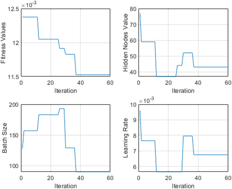
FIGURE 5. BiGRU network hyperparameter search process.
4 Contrastive analysis for forecasting
4.1 Analysis of experimental results
In this section, all experimental results under different prediction steps are discussed in detail. In Tables 3, 4, error indexes of various models under two data sets are given, namely, RMSE, MAE, and MAPE. Subsequently, Tables 3, 4 are analyzed, and the following conclusions can be drawn.
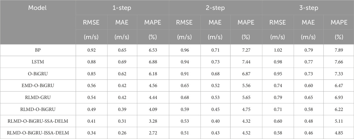
TABLE 3. Results of multi-step prediction on the test data in case of January.
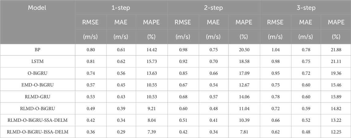
TABLE 4. Results of multi-step prediction on the test data in case of July.
By comparing the error indicators of BP, LSTM, and O-BiGRU in all experimental situations, it can be found that the deep learning network O-BiGRU has lower prediction error in both data sets and prediction horizons, which indicates that BiGRU can obtain better prediction accuracy. Taking the wind speed data of January as an example, the RMSE, MAE, and MAPE indexes obtained by the O-BiGRU model in the one-step, two-step, and three-step prediction are 0.85 m/s, 0.62 m/s, 6.18%; 0.91 m/s, 0.68 m/s, 6.87%; and 0.95 m/s, 0.73 m/s, 7.33%, respectively. The average reduction rate of the MAPE between the other two models and the O-BiGRU model was 11.21% and 9.89%, respectively. Similarly, LSTM, as a deep neural network, has sub-optimal prediction results under the same structure. BP, as a shallow neural network, has the weakest prediction performance due to its weak nonlinear capturing ability, when the model prediction changed from one step to three steps, the MAPE values consistently reached a maximum of 6.53%, 7.27%, and 7.89%, respectively. In addition, this trend is also reflected in the July data set. In the one-step prediction, the O-BiGRU model showed the best performance with an MAPE value of 13.63%. At the same time, when the O-BiGRU was compared to the other two models in the multi-step prediction, the maximum decline rates of MAPE were 7.1% and 10.2%, respectively. It is worth noting that due to the strong non-stationarity of the original wind speed series, the results obtained by using a single model are not satisfactory. Therefore, it is necessary to process the original wind speed sequence to remove the nonlinear limit in the wind speed sequence.
By comparing O-BiGRU and EMD-O-BiGRU, it can be found that data decomposition can greatly improve the prediction performance of the model. In the case of the January prediction, the error indicators obtained by EMD-O-BiGRU in the one-step prediction are 0.56 m/s, 0.42 m/s and 4.56%, respectively, which are 34.12%, 31.25%, and 26.21% lower than those of the single-model O-BiGRU. Meanwhile, by comparing EMD-O-BiGRU and O-BiGRU, the index decline rate of two-step prediction and three-step prediction is 28.57%, 23.53%, and 19.07% and 22.11%, 17.81%, and 11.73%, respectively. At the same time, compared with the EMD-O-BiGRU model, the prediction performance based on RLMD has been comprehensively improved, which indicates that RLMD results may be more suitable for wind speed prediction than EMD. Taking the data in July as an example, RLMD-O-BIGRU showed optimal prediction accuracy, with RMSE values of 0.49, 0.60, and 0.72 for one-step to three-step predictions, respectively. The three error indicators obtained by RLMD-O-BIGRU decreased by 9.49%, 8.70%, and 9.90% on average in the three-step prediction. The RLMD method can effectively alleviate the possible end effect and mode mixing of EMD and further improve the prediction effect.
According to the prediction results of the RLMD-O-BiGRU and RLMD-GRU models, it can be seen that the prediction accuracy of the BiGRU-based model is higher. BiGRU is optimized by the SSA to obtain the best structure, and the structure of the GRU is set to be the same as that of BiGRU, which can make the prediction performance more fair. The former has an average error index decline rate of 11.08% and 10.5% for all prediction steps on the two data sets, respectively. The results show that the bidirectional neural network is superior to the unidirectional network in the learning mode and can extract the features of training data more effectively, thus enhancing the sensitivity of capturing wind speed changes.
The method based on the combination of the error sequence and original sequence can improve the performance of the prediction model to some extent. In this paper, an intelligent algorithm is proposed to optimize the DELM model and form an error correction sector to eliminate the prediction error as much as possible. Taking the data of January as an example, when RLMD-O-BiGRU-SSA-DELM and RLMD-O-BiGRU-ISSA-DELM were compared to the uncorrected model, the average error reduction rates obtained by the model of RLMD-O-BiGRU at three different prediction levels are 18.88%, 10.11%, and 16.86% and 32.48%, 7.62%, and 20.34%, respectively. Similarly, in the July data, compared with the RLMD-O-BiGRU, each indicator of the RLMD-O-BiGRU-SSA-DELM model decreased by 13.27%, 11.82%, and 10.33%, respectively, at different prediction levels. The indexes of RLMD-O-BiGRU-ISSA-DELM decreased by 23.98%, 29.47%, and 16.62%, respectively, at different prediction levels. At the same time, it can be observed that the ISSA has a stronger performance in optimizing the DELM model. For the three-step prediction in all cases, the ISSA-DELM error correction module has an average reduction rate of 4.70%, 5.93%, and 6.21% in RMSE, MAE, and MAPE compared with SSA-DELM, respectively. This trend appears equally in one-step and two-step prediction. Therefore, error correction can improve the overall prediction accuracy of the model. The ISSA has a more obvious positive effect on error correction.
4.2 Analysis and visualization of prediction results
In order to observe the prediction results more directly, the prediction results of wind speed data in January in three prediction steps are shown in Figure 6. The visualized experimental results of the wind speed data in July are shown in Figure 7. A comparison of the predicted and actual values or the error between them is shown on the upper side of the graph. Scatter plots of linear regression curves for some typical models are shown below the graph.
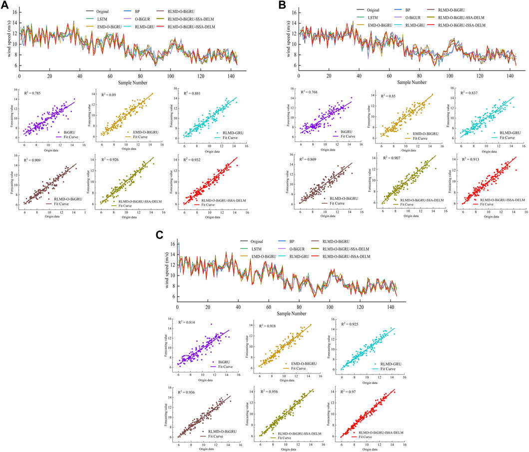
FIGURE 6. (A) Prediction performance of models in the one-step prediction in the case of January. (B) Prediction performance of models in the two-step prediction in the case of January. (C) Prediction performance of models in the three-step prediction in the case of January.
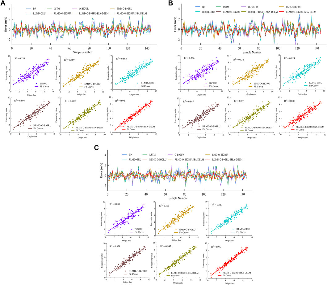
FIGURE 7. (A) Prediction performance of models in the one-step prediction in the case of July. (B) Prediction performance of models in the two-step prediction in the case of July. (C) Prediction performance of models in the three-step prediction in the case of July.
It can be seen from Figures 6, 7 that the model proposed in this paper can fit the real curve well among the three prediction steps. The corresponding error curve fluctuates uniformly around the zero value and has more stable volatility than other models. With the increase in the prediction step, the prediction curve of a single model deviates greatly from the actual value. After data decomposition, the prediction curve of the combined model is relatively stable, and the prediction result after error correction is closest to the real value. From the scatter plots of each model, it can be seen that the proposed method has the most uniform distribution near the regression line, and the average R2 values of the three prediction steps on the two data sets are 0.965, 0.936, and 0.901, respectively, which are the highest among all models. Therefore, the proposed model has the ability of high-precision, multi-step prediction.
In addition, the error indicators represented above are visually presented in Figure 8 to further evaluate the overall performance of all models in the form of radar maps. The variation trend of the single error index in each subgraph with different prediction steps of the model can be seen. Specifically, no matter which subgraph it is in, the proposed model in this article not only has the smallest error measure but also has the smallest variation under the multiple prediction steps. The RLMD-O-BiGRU-SSA-DELM model, which is based on the same framework, provides sub-optimal performance in all experiments. In addition, it can be observed that the prediction performance of the model can be effectively improved after data decomposition. Due to the strong nonlinear processing ability of the deep neural network, the excellent nonlinear fitting ability of the BiGRU model is also verified.
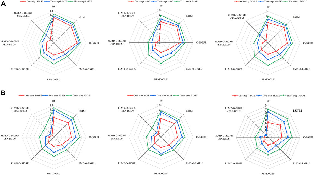
FIGURE 8. Radar map of error index analysis. (A) error analysis of January (B) error analysis of July.
4.3 Further assessment
In addition to using the error index for evaluation in the above model, three other statistical methods are used to analyze the prediction effect of each model in this paper. These include the Diebold–Mariano (DM) test, gray relational analysis (GRA), and predictive stability (FS) (Tian et al., 2018).
The DM test (Diebold and Mariano, 1995) is a hypothesis test proposed by Diebold and Marino. Comparing the calculated DM value with the critical value Zα/2 can reflect whether there are significant differences between the proposed model and other comparison models. When the statistics of the DM value exceed the confidence interval [-Zα/2, Zα/2 ], the null hypothesis is rejected; otherwise, the null hypothesis is accepted.
Table 5 shows all the calculated results, and it can be seen that the lowest DM value is 3.12 among all the single models, so we have 99% reason to believe that the proposed model is better than the single model. Similarly, the minimum value of DM for the single model is 1.67, which is greater than the critical value of 1.64 with a 10% error probability. In general, the proposed model is superior to other comparison models with at least 90% confidence.
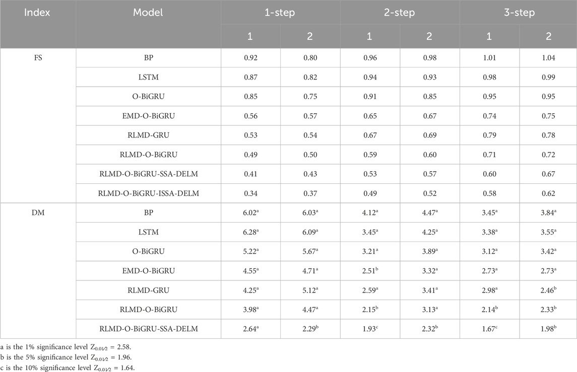
TABLE 5. Results of the statistical test for the related models.
The stability of the prediction is expressed by the standard deviation of the error between the predicted value and the real value, and stability indicators further analyze the prediction ability of the model. It can be seen from Table 5 that with the increase in the prediction step size, the prediction stability becomes worse, but the proposed model always maintains the lowest standard deviation value, which shows that the model has strong prediction stability.
The similarity between the real value and the predicted value is represented by the degree of gray correlation analysis, together with the R2 index, which is shown in Figure 9. It can be seen that when comparing the correlation between the predicted value and the original wind speed through different data sets, the predicted value of the proposed model is most similar to the original curve, with the highest evaluation index, and the correlation value is always maintained as the highest with the increase in the prediction step length, which further verifies the effectiveness of the model.
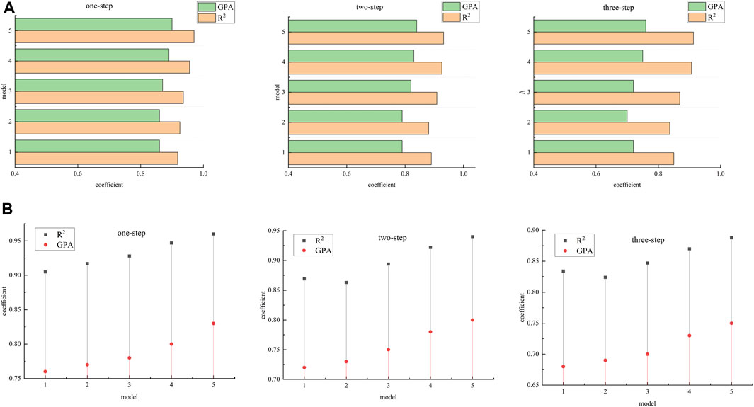
FIGURE 9. Correlation analysis of the model: (A) data analysis of January, (B) data analysis of July. (1: EMD-O-BiGRU; 2: RLMD-GRU; 3: RLMD-O-BiGRU; 4: RLMD-O-BiGRU-SSA-DELM; 5: RLMD-O-BiGRU-ISSA-DELM).
5 Conclusion
With the development of globalization, the development of new energy has become an inevitable choice for sustainable development in all countries. Wind power generation has the advantages of less pollution and being renewable, but its randomness, intermittency, and other characteristics will have a great impact on the power system. In addition, wind speed is an important factor affecting wind power, so accurate and effective establishment of wind speed prediction model is of great significance for the safe and economic operation of the power grid.
In this paper, a novel hybrid prediction model is proposed, which consists of robust mean decomposition, deep neural network, intelligent algorithm, and error correction.
Through the analysis and discussion of the actual data of a region in central China, the superiority of the model is verified. (1) The RLMD method can effectively solve the problems of end effect and mode mixing. Compared with the classical EMD, this method can more effectively solve the non-stationarity and nonlinearity problems of the original data. (2) The SSA is used to search hyperparameters in deep learning networks, overcoming the blindness of experience selection and ensuring the quality of prediction. (3) Based on the traditional SSA, an improved SSA is proposed, and an ISSA-DELM error correction model is established. The results show that error correction has a positive impact on improving the initial prediction accuracy. (4) Through the analysis of various error indicators and statistical indicators on different data sets, it is verified that the proposed model has good prediction performance.
Although the hybrid model proposed in this paper has a better prediction effect, there are still some challenges. Due to the difficulty of collecting original data, this paper only used data from one region. In the process of data acquisition, different sampling frequencies make the data show different characteristics of chaos. Therefore, in future work, the diversity of data should be considered to fully verify the applicability and prediction ability of the model. Meanwhile, in this study, the training data only included historical data and did not take into account other meteorological factors. In fact, wind speed is affected by temperature, pressure, humidity, and other factors, and the interweaving of these factors leads to significant nonlinear characteristics of wind speed change. Therefore, the next step should be to establish a multi-input model, fully extract the features between the data, and dig into the deep law of wind speed change. In addition, in view of the significant improvement in the prediction effect of the decomposition methods, improving the decomposition algorithm is a promising research direction to achieve accurate decomposition of the initial wind speed series.
Data availability statement
The raw data supporting the conclusions of this article will be made available by the authors, without undue reservation.
Author contributions
JL: conceptualization, methodology, software, and writing–original draft. ML: project administration, validation, and writing–review and editing. LW: validation and writing–review and editing.
Funding
The author(s) declare that no financial support was received for the research, authorship, and/or publication of this article.
Conflict of interest
Author JL was employed by Hangzhou Digital Energy and Low Carbon Technology Co., Ltd.
The remaining authors declare that the research was conducted in the absence of any commercial or financial relationships that could be construed as a potential conflict of interest.
Publisher’s note
All claims expressed in this article are solely those of the authors and do not necessarily represent those of their affiliated organizations, or those of the publisher, the editors, and the reviewers. Any product that may be evaluated in this article, or claim that may be made by its manufacturer, is not guaranteed or endorsed by the publisher.
References
Adnan, R. M., Mostafa, R. R., Kisi, O., Yaseen, Z. M., Shahid, S., and Zounemat-Kermani, M. (2021). Improving streamflow prediction using a new hybrid ELM model combined with hybrid particle swarm optimization and grey wolf optimization. Knowledge-Based Syst. 230, 19. doi:10.1016/j.knosys.2021.107379
Ahmadpour, A., and Farkoush, S. G. (2020). Gaussian models for probabilistic and deterministic Wind Power Prediction: wind farm and regional. Int. J. Hydrogen Energy 45 (51), 27779–27791. doi:10.1016/j.ijhydene.2020.07.081
Alhussan, A. A., Farhan, A. K., Abdelhamid, A. A., El-Kenawy, E. M., Ibrahim, A., and Khafaga, D. S. (2023). Optimized ensemble model for wind power forecasting using hybrid whale and dipper-throated optimization algorithms. Front. Energy Res. 11, 17. doi:10.3389/fenrg.2023.1174910
An, G. Q., Chen, L. B., Tan, J. X., Jiang, Z. Y., Li, Z., and Sun, H. X. (2022). Ultra-short-term wind power prediction based on PVMD-ESMA-DELM. Energy Rep. 8, 8574–8588. doi:10.1016/j.egyr.2022.06.079
Ates, K. T. (2023). Estimation of short-term power of wind turbines using artificial neural network (ANN) and swarm intelligence. Sustainability 15 (18), 13572. doi:10.3390/su151813572
Bommidi, B. S., Kosana, V., Teeparthi, K., and Madasthu, S. (2023). Hybrid attention-based temporal convolutional bidirectional LSTM approach for wind speed interval prediction. Environ. Sci. Pollut. Res. 30 (14), 40018–40030. doi:10.1007/s11356-022-24641-x
Chi, D. W., and Yang, C. Z. (2023). Wind power prediction based on WT-BiGRU-attention-TCN model. Front. Energy Res. 11, 12. doi:10.3389/fenrg.2023.1156007
Cho, K., van Merrienboer, B., Gulcehre, C., Bahdanau, D., Bougares, F., Schwenk, H., et al. (2014). Learning phrase representations using RNN encoder-decoder for statistical machine translation. Arxiv. Available at: https://doi.org/10.48550/arXiv.1406.1078.
Diebold, F. X., and Mariano, R. S. (1995). Comparing predictive accuracy. J. Bus. Econ. Statistics 13 (3), 253–263. doi:10.1080/07350015.1995.10524599
Ding, L., Bai, Y. L., Liu, M. D., Fan, M. H., and Yang, J. (2022). Predicting short wind speed with a hybrid model based on a piecewise error correction method and Elman neural network. Energy 244, 122630. doi:10.1016/j.energy.2021.122630
Ding, S. F., Zhang, N., Xu, X. Z., Guo, L. L., and Zhang, J. (2015). Deep extreme learning machine and its application in EEG classification. Math. Problems Eng. 2015, 129021–129111. doi:10.1155/2015/129021
Erdem, E., and Shi, J. (2011). ARMA based approaches for forecasting the tuple of wind speed and direction. Appl. Energy 88 (4), 1405–1414. doi:10.1016/j.apenergy.2010.10.031
Fu, W. L., Fang, P., Wang, K., Li, Z. X., Xiong, D. Z., and Zhang, K. (2021). Multi-step ahead short-term wind speed forecasting approach coupling variational mode decomposition, improved beetle antennae search algorithm-based synchronous optimization and Volterra series model. Renew. Energy 179, 1122–1139. doi:10.1016/j.renene.2021.07.119
Gao, B. X., Huang, X. Q., Shi, J. S., Tai, Y. H., and Zhang, J. (2020). Hourly forecasting of solar irradiance based on CEEMDAN and multi-strategy CNN-LSTM neural networks. Renew. Energy 162, 1665–1683. doi:10.1016/j.renene.2020.09.141
Gao, R. B., Du, L., Duru, O., and Yuen, K. F. (2021). Time series forecasting based on echo state network and empirical wavelet transformation. Appl. Soft Comput. 102, 107111. doi:10.1016/j.asoc.2021.107111
Han, Y., Tong, X., Shi, S., Li, F., and Deng, Y. (2023). Ultra-short-term wind power interval prediction based on hybrid temporal inception convolutional network model. Electr. Power Syst. Res. 217, 109159. doi:10.1016/j.epsr.2023.109159
Hoolohan, V., Tomlin, A. S., and Cockerill, T. (2018). Improved near surface wind speed predictions using Gaussian process regression combined with numerical weather predictions and observed meteorological data. Renew. Energy 126, 1043–1054. doi:10.1016/j.renene.2018.04.019
Hu, H. Z., Li, Y. Y., Zhang, X. P., and Fang, M. G. (2022). A novel hybrid model for short-term prediction of wind speed. Pattern Recognit. 127, 108623. doi:10.1016/j.patcog.2022.108623
Huang, G. B., Zhu, Q. Y., and Siew, C. K. (2004). “Extreme learning machine: a new learning scheme of feedforward neural networks,” in 2004 IEEE International Joint Conference on Neural Networks (IEEE Cat. No.04CH37541), Budapest, Hungary, 25-29 July 2004, 985–990.
Jia, H., Liu, Q., Liu, Y., Wang, S., and Wu, D. (2023). Hybrid Aquila and Harris hawks optimization algorithm with dynamic opposition-based learning. CAAI Trans. Intelligent Syst. 18 (1), 104–116.
Jiang, Z. Y., Che, J. X., and Wang, L. N. (2021). Ultra-short-term wind speed forecasting based on EMD-VAR model and spatial correlation. Energy Convers. Manag. 250, 114919. doi:10.1016/j.enconman.2021.114919
Jiao, X. G., Zhang, D. Y., Wang, X., Tian, Y. B., Liu, W. F., and Xin, L. P. (2023). Wind speed prediction based on error compensation. Sensors 23 (10), 4905. doi:10.3390/s23104905
Karaku, O., Kuruolu, E. E., and Altnkaya, M. A. (2017). One-day ahead wind speed/power prediction based on polynomial autoregressive model. IET Renew. Power Gener. 11 (11), 1430–1439. doi:10.1049/iet-rpg.2016.0972
Li, X. C., Ma, X. F., Xiao, F. C., Xiao, C., Wang, F., and Zhang, S. C. (2022). Time-series production forecasting method based on the integration of bidirectional gated recurrent unit (Bi-GRU) network and sparrow search algorithm (SSA). J. Petroleum Sci. Eng. 208, 109309. doi:10.1016/j.petrol.2021.109309
Liang, X. H., Hu, F. H., Li, X., Zhang, L., Feng, X., and Abu Gunmi, M. (2023). Ultra-short-term wind speed prediction based on deep spatial-temporal residual network. J. Renew. Sustain. Energy 15 (4), 14. doi:10.1063/5.0153298
Lin, S. M., Wang, J., Xu, X. F., Tan, H., Shi, P. M., and Li, R. X. (2023). SWSA transformer: a forecasting method of ultra-short-term wind speed from an offshore wind farm using global attention mechanism. J. Renew. Sustain. Energy 15 (4), 16. doi:10.1063/5.0153511
Liu, H., and Chen, C. (2019). Multi-objective data-ensemble wind speed forecasting model with stacked sparse autoencoder and adaptive decomposition-based error correction. Appl. Energy 254, 113686. doi:10.1016/j.apenergy.2019.113686
Liu, L., Liu, J. C., Ye, Y., Liu, H., Chen, K., Li, D., et al. (2023). Ultra-short-term wind power forecasting based on deep Bayesian model with uncertainty. Renew. Energy 205, 598–607. doi:10.1016/j.renene.2023.01.038
Liu, M., Cao, Z., Zhang, J., Wang, L., Huang, C., and Luo, X. (2020). Short-term wind speed forecasting based on the Jaya-SVM model. Int. J. Electr. Power Energy Syst. 121, 106056. doi:10.1016/j.ijepes.2020.106056
Liu, Z. L., Jin, Y. Q., Zuo, M. J., and Feng, Z. P. (2017). Time-frequency representation based on robust local mean decomposition for multicomponent AM-FM signal analysis. Mech. Syst. Signal Process. 95, 468–487. doi:10.1016/j.ymssp.2017.03.035
López, G., and Arboleya, P. (2022). Short-term wind speed forecasting over complex terrain using linear regression models and multivariable LSTM and NARX networks in the Andes Mountains, Ecuador. Renew. Energy 183, 351–368. doi:10.1016/j.renene.2021.10.070
Lv, M. Z., Wang, J. Z., Niu, X. S., and Lu, H. Y. (2022). A newly combination model based on data denoising strategy and advanced optimization algorithm for short-term wind speed prediction. J. Ambient Intell. Humaniz. Comput. 20, 8271–8290. doi:10.1007/s12652-021-03595-x
Mirjalili, S., Gandomi, A. H., Mirjalili, S. Z., Saremi, S., Faris, H., and Mirjalili, S. M. (2017). Salp Swarm Algorithm: a bio-inspired optimizer for engineering design problems. Adv. Eng. Softw. 114, 163–191. doi:10.1016/j.advengsoft.2017.07.002
Mirjalili, S. J. N. C.Applications (2016). Dragonfly algorithm: a new meta-heuristic optimization technique for solving single-objective, discrete, and multi-objective problems. Neural Comput Applic 27 (4), 1053–1073. doi:10.1007/s00521-015-1920-1
Niu, Z. W., Yu, Z. Y., Tang, W. H., Wu, Q. H., and Reformat, M. (2020). Wind power forecasting using attention-based gated recurrent unit network. Energy 196, 117081. doi:10.1016/j.energy.2020.117081
Peng, S. B., Chen, R. L., Yu, B., Xiang, M., Lin, X. G., and Liu, E. B. (2021). Daily natural gas load forecasting based on the combination of long short term memory, local mean decomposition, and wavelet threshold denoising algorithm. J. Nat. Gas Sci. Eng. 95, 104175. doi:10.1016/j.jngse.2021.104175
Sabat, N. K., Nayak, R., Srivastava, H., Pati, U. C., and Das, S. K. (2023). Prediction of meteorological parameters using statistical time series models: a case study. Int. J. Glob. Warming 31 (1), 128–149. doi:10.1504/ijgw.2023.133547
Shang, Z. H., Li, M., Chen, Y. H., Li, C. H., Yang, Y., and Li, L. (2022). A novel model based on multiple input factors and variance reciprocal: application on wind speed forecasting. Soft Comput. 26 (17), 8857–8877. doi:10.1007/s00500-021-06661-w
Smith, J. S. (2005). The local mean decomposition and its application to EEG perception data. J. R. Soc. Interface 2 (5), 443–454. doi:10.1098/rsif.2005.0058
Syama, S., Ramprabhakar, J., Anand, R., and Guerrero, J. M. (2023). A hybrid extreme learning machine model with levy flight chaotic whale optimization algorithm for wind speed forecasting. Results Eng. 19, 101274. doi:10.1016/j.rineng.2023.101274
Tang, Z., Zhao, G., Cao, S., Ouyang, T., Mu, Z., and Pang, X. (2021). A dataanalystic based hybrid wind direction prediction algorithm. Acta Energiae Solaris Sin. 42 (9), 349–356. doi:10.19912/j.0254-0096.tynxb.2020-0119
Tian, C. S., Hao, Y., and Hu, J. M. (2018). A novel wind speed forecasting system based on hybrid data preprocessing and multi-objective optimization. Appl. Energy 231, 301–319. doi:10.1016/j.apenergy.2018.09.012
Tian, Z. D. (2020a). Backtracking search optimization algorithm-based least square support vector machine and its applications. Eng. Appl. Artif. Intell. 94, 103801. doi:10.1016/j.engappai.2020.103801
Tian, Z. D. (2020b). Short-term wind speed prediction based on LMD and improved FA optimized combined kernel function LSSVM. Eng. Appl. Artif. Intell. 91, 103573. doi:10.1016/j.engappai.2020.103573
Tian, Z. D. (2021). Modes decomposition forecasting approach for ultra-short-term wind speed. Appl. Soft Comput. 105, 107303. doi:10.1016/j.asoc.2021.107303
Tian, Z. D., and Chen, H. (2021a). Multi-step short-term wind speed prediction based on integrated multi-model fusion. Appl. Energy 298, 117248. doi:10.1016/j.apenergy.2021.117248
Tian, Z. D., and Chen, H. (2021b). A novel decomposition-ensemble prediction model for ultra-short-term wind speed. Energy Convers. Manag. 248, 114775. doi:10.1016/j.enconman.2021.114775
Tian, Z. D., Li, H., and Li, F. H. (2021). A combination forecasting model of wind speed based on decomposition. Energy Rep. 7, 1217–1233. doi:10.1016/j.egyr.2021.02.002
Tian, Z. D., Li, S. J., and Wang, Y. H. (2020). A prediction approach using ensemble empirical mode decomposition-permutation entropy and regularized extreme learning machine for short-term wind speed. Wind Energy 23 (2), 177–206. doi:10.1002/we.2422
Tuerxun, W., Xu, C., Guo, H. Y., Guo, L., Zeng, N. M., and Gao, Y. S. (2022). A wind power forecasting model using LSTM optimized by the modified bald eagle search algorithm. Energies 15 (6), 2031. doi:10.3390/en15062031
Wang, C. H., Zhao, Q. G., and Tian, R. (2023a). Short-term wind power prediction based on a hybrid markov-based PSO-BP neural network. Energies 16 (11), 4282. doi:10.3390/en16114282
Wang, H., Xiong, M., Chen, H. F., and Liu, S. M. (2022). Multi-step ahead wind speed prediction based on a two-step decomposition technique and prediction model parameter optimization. Energy Rep. 8, 6086–6100. doi:10.1016/j.egyr.2022.04.045
Wang, J. Z., Guo, H. G., Li, Z. W., Song, A. Y., and Niu, X. S. (2023b). Quantile deep learning model and multi-objective opposition elite marine predator optimization algorithm for wind speed prediction. Appl. Math. Model. 115, 56–79. doi:10.1016/j.apm.2022.10.052
Wang, X., Wang, W., and Wang, Y. (2013). “An adaptive bat algorithm,” in Intelligent computing theories and technology. ICIC 2013 (Berlin, Heidelberg: Springer).
Xiang, L., Li, J. X., Hu, A. J., and Zhang, Y. (2020). Deterministic and probabilistic multi-step forecasting for short-term wind speed based on secondary decomposition and a deep learning method. Energy Convers. Manag. 220, 113098. doi:10.1016/j.enconman.2020.113098
Yan, X. A., Liu, Y., Xu, Y. D., and Jia, M. P. (2020). Multistep forecasting for diurnal wind speed based on hybrid deep learning model with improved singular spectrum decomposition. Energy Convers. Manag. 225, 113456. doi:10.1016/j.enconman.2020.113456
Yao, X., Liu, Y., and Lin, G. M. (1999). Evolutionary programming made faster. Ieee Trans. Evol. Comput. 3 (2), 82–102. doi:10.1109/4235.771163
Ying, C. T., Wang, W. Q., Yu, J., Li, Q., Yu, D. H., and Liu, J. H. (2023). Deep learning for renewable energy forecasting: a taxonomy, and systematic literature review. J. Clean. Prod. 384, 135414. doi:10.1016/j.jclepro.2022.135414
Yuan, X., Tan, Q., Lei, X., Yuan, Y., and Wu, X. (2017). Wind power prediction using hybrid autoregressive fractionally integrated moving average and least square support vector machine. Energy 129 (Jun.15), 122–137. doi:10.1016/j.energy.2017.04.094
Yunus, K., Thiringer, T., and Chen, P. Y. (2016). ARIMA-based frequency-decomposed modeling of wind speed time series. IEEE Trans. Power Syst. 31 (4), 2546–2556. doi:10.1109/tpwrs.2015.2468586
Zhang, C., Hua, L., Ji, C. L., Nazir, M. S., and Peng, T. (2022a). An evolutionary robust solar radiation prediction model based on WT-CEEMDAN and IASO-optimized outlier robust extreme learning machine. Appl. Energy 322, 119518. doi:10.1016/j.apenergy.2022.119518
Zhang, C., Ma, H. X., Hua, L., Sun, W., Nazir, M. S., and Peng, T. (2022b). An evolutionary deep learning model based on TVFEMD, improved sine cosine algorithm, CNN and BiLSTM for wind speed prediction. Energy 254, 124250. doi:10.1016/j.energy.2022.124250
Zhang, D., Chen, Z., Xin, Z., Zhang, H., and Yan, W. (2020). Salp swarm algorithm based on craziness and adaptive. Control Decis. 35 (9), 2112–2120. doi:10.13195/j.kzyjc.2019.0012
Zhang, Y. G., Han, J. Y., Pan, G. F., Xu, Y., and Wang, F. (2021). A multi-stage predicting methodology based on data decomposition and error correction for ultra-short-term wind energy prediction. J. Clean. Prod. 292, 125981. doi:10.1016/j.jclepro.2021.125981
Zhang, Y. G., and Wang, S. Q. (2022). An innovative forecasting model to predict wind energy. Environ. Sci. Pollut. Res. 29 (49), 74602–74618. doi:10.1007/s11356-022-20971-y
Zhang Y G, Y. G., Zhang, J. H., Yu, L. Y., Pan, Z. Y., Feng, C. Y., Sun, Y. Q., et al. (2022). A short-term wind energy hybrid optimal prediction system with denoising and novel error correction technique. Energy 254, 124378. doi:10.1016/j.energy.2022.124378
Keywords: wind speed prediction, data decomposition, bidirectional gated recurrent unit, salp swarm algorithm, deep extreme learning machine, error correction
Citation: Li J, Liu M and Wen L (2024) Forecasting model for short-term wind speed using robust local mean decomposition, deep neural networks, intelligent algorithm, and error correction. Front. Energy Res. 11:1336675. doi: 10.3389/fenrg.2023.1336675
Received: 11 November 2023; Accepted: 28 December 2023;
Published: 25 January 2024.
Edited by:
Juan P. Amezquita-Sanchez, Autonomous University of Queretaro, MexicoReviewed by:
Zhongda Tian, Shenyang University of Technology, ChinaCarlos Andrés Perez Ramirez, Autonomous University of Queretaro, Mexico
Copyright © 2024 Li, Liu and Wen. This is an open-access article distributed under the terms of the Creative Commons Attribution License (CC BY). The use, distribution or reproduction in other forums is permitted, provided the original author(s) and the copyright owner(s) are credited and that the original publication in this journal is cited, in accordance with accepted academic practice. No use, distribution or reproduction is permitted which does not comply with these terms.
*Correspondence: Minghao Liu, Y2hpbmFfYWxtb3N0QDE2My5jb20=