Research on micro/nano scale 3D reconstruction based on scanning electron microscope

Scanning electron microscopy (SEM) has an important application in the petroleum field, which is often used to analyze the microstructure of reservoir rocks, etc. Most of these analyses are based on two-dimensional images. In fact, SEM can carry out micro-nano scale three-dimensional measurement, and three-dimensional models can provide more accurate information than two-dimensional images. Among the commonly used SEM 3D reconstruction methods, parallax depth mapping is the most commonly used method. Multiple SEM images can be obtained by continuously tilting the sample table at a certain Angle, and multiple point clouds can be generated according to the parallax depth mapping method, and a more complete point clouds recovery can be achieved by combining the point clouds registration. However, the root mean square error of the point clouds generated by this method is relatively large and unstable after participating in point clouds registration. Therefore, this paper proposes a new method for generating point clouds. Firstly, the sample stage is rotated by a certain angle to obtain two SEM images. This operation makes the rotation matrix a known quantity. Then, based on the imaging model, an equation system is constructed to estimate the unknown translation parameters, and finally, triangulation is used to obtain the point clouds. The method proposed in this paper was tested on a publicly available 3D SEM image set, and the results showed that compared to the disparity depth mapping method, the point clouds generated by our method showed a significant reduction in root mean square error and relative rotation error in point clouds registration.

1 Introduction

One of the main drawbacks of optical microscopes is their limitations in resolving finer details. Scanning electron microscopes (SEM) use electron imaging, and the wavelength of electrons is much smaller than that of photons, easily achieving magnifications of tens or even hundreds of thousands of times. However, SEM can only obtain 2D images and cannot directly generate 3D shapes. Compared to 2D images, three-dimensional structures can provide more information for many micro research fields. For example, SEM has important applications in the petroleum field, (Zhu, 2013; Liu et al., 2023; Wu et al., 2023), used SEM in the analysis of the micro pore structure of reservoir rocks. Yao used SEM combined with deep learning based image processing to characterize the nanoscale pore structure of rock debris (Yao et al., 2022). Scholars have also used SEM to observe and analyze the microstructure of solid/oil well cement stone (Li et al., 2016; Zhang et al., 2013; Song et al., 2017; Song et al., 2020). Munawar used optical polarization microscopy in transmission mode to document the whole-rock mineralogy, diagenetic relationships, porosity characteristics and clay occurrences in the pores of these samples (Munawar et al., 2018a). Wang used focused ion beam scanning electron microscopy (FIB-SEM) to reconstruct the internal organic matter pores of shale using a three-dimensional-slicing-imaging reconstruction technology route, but its literature also indicated that FIB can cause damage to the sample during the slicing process, which is a destructive analysis method (Wang et al., 2019). Munawar mentions that micro-CT imaging has certainly some limitations concerning sample size and resolution (Munawar et al., 2018b). It is reliable to captures micron scale features, whereas it is not possible for micro-CT to capture nanometer scale features (Munawar et al., 2018b; Luo et al., 2022; Ji et al., 2015). There are scholars used X-ray CT to perform three-dimensional measurements on carbonate rock and sandstone sample (Munawar et al., 2021). A series of two-dimensional slices stack into a 3D image. Data are arranged in an array of pixels in the two-dimensional slice. A pixel in the third dimension makes it three-dimensional volume which is a voxel. This is, the distance between two consecutive slices is a voxel. The 3D model formed by stacking sliced images is a discrete model, but compared to FIBSEM, this is a reconstruction method for non-destructive samples. The resolution of the new scanning electron microscope can reach 1 nm. Based on SEM 3D reconstruction, nanoscale, spatially continuous 3D models can be obtained, which is helpful for calculating porosity. There are many scholars also use SEM equipment in petroleum energy research (Huang et al., 2023a; Huang et al., 2023b; Tan et al., 2023; Tan et al., 2020; Huang et al., 2020; Huang et al., 2022). SEM can provide high-resolution images without damaging the sample. If standard SEM machines can be used to restore the microscopic three-dimensional structure of samples such as rocks in the above research, it will provide more information for analyzing pore structure, material toughness, etc. without damage. In order to effectively measure and visualize the three-dimensional structure of microscopic samples, many scholars have been trying to convert scanning electron microscopy into microscopic three-dimensional measurement tools.

Currently, the commonly used 3D reconstruction algorithms under scanning electron microscopy include the Photometric Stereo (PS) method (Ikeuchi, 1981; Basri et al., 2007; Goldman et al., 2010). As shown in Figure 1, in the PS based method, the sample stage and detector of the scanning electron microscope remain stationary, providing illumination in different directions to the sample stage. From a single perspective, the detector captures a set of 2D images in different lighting directions and quickly calculates the 3D geometric shape of the SEM sample. However, since only one perspective is used, it is not possible to create a complete point clouds, and the PS method requires illumination from different directions on the sample stage, making it difficult to have such additional lighting conditions using standard scanning electron microscopy machines, which increases equipment costs and limitations.

FIGURE 1

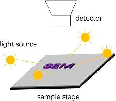
FIGURE 1. Photometric Stereo (PS) method.

(Wang et al., 2013) used SFS (shape from shading) technology to analyze the grayscale information of a single top view SEM image, and ultimately reconstructed the three-dimensional surface structure. However, due to the fixed perspective, a complete point clouds cannot be obtained.

(Ding et al., 2019) adopted a nanorobot system to automatically capture a set of scanning electron microscope images along a linear path with a fixed step size, and used light field theory to reconstruct the three-dimensional surface model of SEM samples. As shown in Figure 2A, the sample is fixed on the sample stage via either glue, tape or customized grippers according to sample properties. After assembling the nano-robotic manipulation system inside SEM, the linear positioner is utilized to move step by step along x-axis with a fixed step size, and one SEM image is taken after each step. Figure 2B shows the SEM images obtained at each step. However, not all SEM devices are equipped with nanorobot systems, and the step accuracy of nanorobot systems is limited, requiring a large number of images to be captured.

FIGURE 2

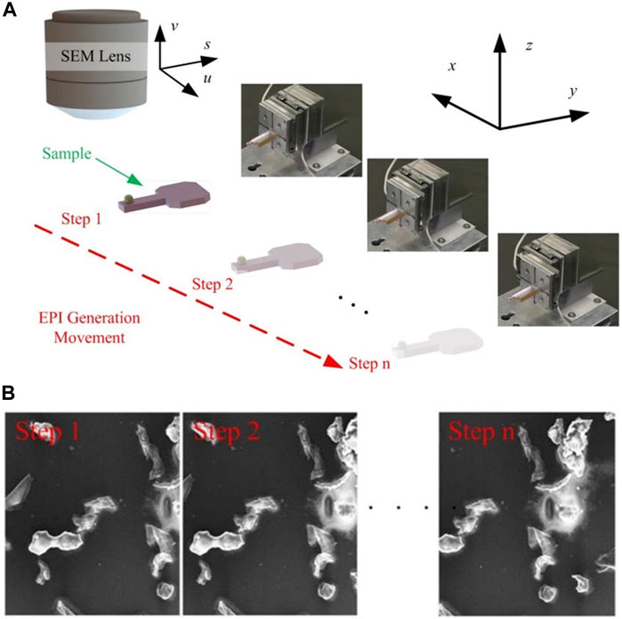
FIGURE 2. (A) The movement process of nanorobots (B) Image obtained step by step.

Tafti et al., 2015; Tafti et al., 2016 designed an optimized, parameter adaptive, and intelligent multi view method, 3DSEM++, for 3D surface reconstruction of SEM images. He also publicly and freely provided a 3D SEM image set, which is derived from Tafti’s publicly available image set. Some scholars have studied the use of optical measurement software for three-dimensional reconstruction of SEM images (Eulitz and Reiss, 2015; Kareiva et al., 2015), but optical measurement software often does not consider the imaging characteristics of SEM itself, and generally requires images to contain EXIF information and camera model, which SEM images often do not have.

The parallax depth mapping method (Samak et al., 2007; Baghaie et al., 2017; Yi et al., 2019; Bian, 2020) is the simplest and fastest way to obtain the three-dimensional structure of SEM samples. As shown in Figure 3A, θ is the rotation angle, and the relationship between disparity d and depth h is given by a formula.

FIGURE 3

FIGURE 3. (A) The principle of disparity depth mapping and the rotation method of the sample stage (B) Parallax depth mapping to obtain multiple point clouds, and then point clouds registration.

$h=\frac{d}{2*\sin \theta }$

, by rotating the sample stage at a certain angle to obtain two SEM images, a point clouds can be created based on parallax. However, since parallax depth mapping can only use two images at once, it is also not possible to create a complete point clouds. In response to the insufficient integrity of the point clouds reconstructed by the disparity depth mapping method, Rehman used disparity depth mapping combined with point clouds registration to achieve multi view SEM 3D reconstruction [Rehman, 2018]. As shown in Figure 3B, multiple point clouds are obtained by using the parallax depth mapping multiple times, and then point clouds registration is performed

Liu used incremental motion recovery structure (SFM) to perform 3D reconstruction of the SEM image sequence of the Drosophila head, and successfully restored the point clouds (Liu, 2018). SFM uses singular value decomposition of the essential matrix to obtain initial rotation and translation parameters. Unfortunately, this method yields poor results on the image set presented in this paper.

This article improves the shortcomings of the aforementioned SEM based 3D reconstruction methods, such as a single perspective, equipment cost limitations, lack of consideration for SEM imaging characteristics, and time consumption. It proposes a method for restoring the detector pose, which is different from traditional essential matrix singular value decomposition. It uses imaging equations of multiple image points to form a system of equations, analyzes the known internal and external parameters in the imaging model, and calculates the motion parameters of the position. Triangulation is used to generate point clouds of different parts of the microscopic sample, and then point clouds registration is combined to obtain a more complete point clouds. Thus, standard SEM machines can be used to achieve three-dimensional reconstruction of microscopic samples from multiple perspectives.

The content of this article is arranged as follows. The first section is an introduction, which introduces the commonly used methods and shortcomings of three-dimensional reconstruction of microscopic samples under SEM.

Section 2 will introduce the publicly available 3D SEM image set and point out that there are some known conditions in this image set that are beneficial for subsequent calibration work.

Section 3 will introduce the SEM three-dimensional measurement model. When the magnification of the SEM exceeds 1,000, the SEM imaging process is similar to a double telecentric lens. At this point, the parallel projection model is more suitable for the SEM imaging model. Then, based on the publicly available 3D SEM image set, a motion parameter estimate method between SEM image sequences suitable for this image set is derived.

Section 4 will present a more specific experimental process and results.

In Section 5, the evaluation indicators for point clouds registration, including root mean square error and relative rotation error, will be introduced. Due to the fact that the relative translation motion in relative transformation does not have a true value as a reference, relative translation error cannot be used as an evaluation indicator. Under these indicators, the registration results of our method will be compared and analyzed with those of the disparity depth mapping method.

Section 6 will provide the discussion and conclusion of this article.

2 3D SEM image set

The 3D SEM image set used in this article is from the publicly available SEM image set by Tafti, available at the website https://dataverse.harvard.edu/dataset.xhtml?persistentId=doi:10.7910/DVN/HVBW0Q#__sid=js0, the characteristic of this image set is that, as shown in Figure 3A, in the image sequence, the Y-axis of the sample stage itself is used as the rotation axis, and a fixed angle is rotated around that axis θ to obtain the next image, during the actual shooting process, this rotation operation will be continuously performed to obtain multiple SEM images. The rotation angle θ will serve as an important rotational motion parameter in the imaging model.

Although the actual operation process involves the sample stage rotating around its Y-axis while the imaging plane remains stationary, it can be seen that the sample stage remains stationary and the imaging plane rotates around the sample stage because the motion is relative. Figure 3B shows the equivalent shooting process of SEM images of “ Pollen grain from Brassica rapa ” in the image set.

This publicly available 3DSEM image set was obtained using standard SEM equipment, and its special motion method is to apply the disparity depth mapping method. Many scholars have also used this image set to conduct extensive research based on disparity depth mapping. Among them, Rehman added point clouds registration to it, enabling all SEM images to be used and obtaining a more complete point clouds (Rehman, 2018). However, the above studies are all based on disparity depth mapping. In fact, this image set can use calibration methods to estimate motion parameters, and then use triangulation to recover point clouds. Section 5 will compare these two methods.

3 SEM 3D measurement model

3.1 SEM imaging model

As shown in Figure 4, the SEM imaging process essentially involves hitting the surface of the sample with an electron beam, and then sampling by the detector to obtain the grayscale information of each sampling point. This process can be seen as a three-dimensional to two-dimensional mapping (Liu, 2018). Therefore, the SEM imaging process is also regarded by many scholars as a projection transformation. SEM expert Reimer once pointed out that the SEM imaging process can be approximated as a perspective projection process (Reimer, 1985), but in recent years, research has shown that the imaging model of electronic imaging systems is different under different magnifications: when the magnification is low, the field of view and angle of view are large, and the classical perspective projection model can be used to model the imaging system, when the magnification is large, the field of view and angle of view are both very small, and the imaging process is approximately parallel projection.

FIGURE 4

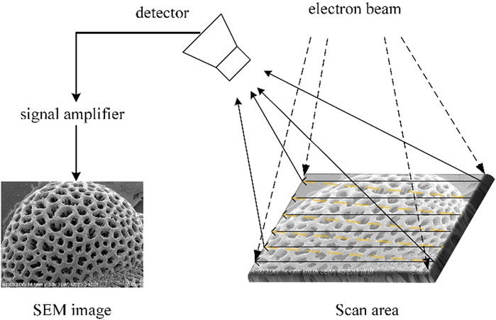
FIGURE 4. Schematic diagram of SEM imaging process.

Due to the fact that the SEM imaging model depends on the size of the magnification, finding an appropriate critical value has become the key to studying two different projection models. (Sutton et al., 2007). conducted extensive research on the SEM projection model and obtained a widely recognized critical value, which is that when the magnification is higher than 1,000x, the projection model can be approximated as a parallel projection, When the magnification is below 1,000x, the projection model can be considered as a transmission projection. As shown in Figure 5.

FIGURE 5

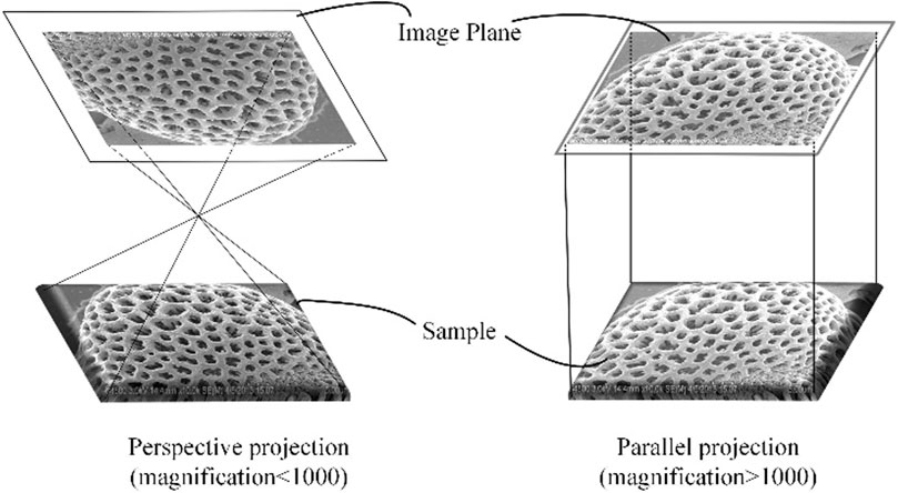
FIGURE 5. SEM imaging model under different magnification.

The magnification of the 3D SEM image set used in this article exceeds 1,000x, so this article mainly studies 3D reconstruction under parallel projection models. The formula for the parallel projection imaging model is as follows:

The mathematical model of image points [u v] and corresponding world points [X Y Z] is as follows (Liu, 2018):

$\left[\begin{array}{c}u\\ v\\ 1\end{array}\right]=\left[\begin{array}{ccc}a& 0& 0\\ 0& a& 0\\ 0& 0& 1\end{array}\right]\left[\begin{array}{cc}\begin{array}{cc}1& 0\end{array}& \begin{array}{cc}0& 0\end{array}\\ \begin{array}{cc}0& 1\end{array}& \begin{array}{cc}0& 0\end{array}\\ \begin{array}{cc}0& 0\end{array}& \begin{array}{cc}0& 1\end{array}\end{array}\right]\left[\begin{array}{cc}\begin{array}{cc}\begin{array}{c}{r}_{11}\\ r_{21}\\ \begin{array}{c}{r}_{31}\\ 0\end{array}\end{array}& \begin{array}{c}{r}_{12}\\ r_{22}\\ \begin{array}{c}{r}_{32}\\ 0\end{array}\end{array}\end{array}& \begin{array}{cc}\begin{array}{c}{r}_{13}\\ r_{23}\\ \begin{array}{c}{r}_{33}\\ 0\end{array}\end{array}& \begin{array}{c}{t}_x\\ t_y\\ \begin{array}{c}{t}_z\\ 1\end{array}\end{array}\end{array}\end{array}\right]\left[\begin{array}{c}\begin{array}{c}X\\ Y\end{array}\\ \begin{array}{c}Z\\ 1\end{array}\end{array}\right],(1)$

The matrix where a is located in equation 1 is the SEM internal matrix. Due to the characteristics of parallel projection, the main point of the image in the internal matrix is 0, and a is the scale factor between pixel size and actual scale, it can be calculated from the dpi of the SEM image and the scale bar on the image. The dpi of the image represents the number of pixels per inch of length, and SEM images usually provide scale bar and other information at the bottom of the image, r_ii are the element within the rotation matrix, t_x, t_y, and t_z are the elements within the translation vector. The two together form the SEM external matrix. It can be observed that the third row of the rotation matrix r_3i and the third component of the translation vector t_z do not affect the imaging process, as they are multiplied by 0. Therefore, equation 1 is simplified as follows:

$\left[\begin{array}{c}u\\ v\\ 1\end{array}\right]=\left[\begin{array}{ccc}a& 0& 0\\ 0& a& 0\\ 0& 0& 1\end{array}\right]\left[\begin{array}{cc}\begin{array}{cc}\begin{array}{c}{r}_{11}\\ r_{21}\\ 0\end{array}& \begin{array}{c}{r}_{12}\\ r_{22}\\ 0\end{array}\end{array}& \begin{array}{cc}\begin{array}{c}{r}_{13}\\ r_{23}\\ 0\end{array}& \begin{array}{c}{t}_x\\ t_y\\ 1\end{array}\end{array}\end{array}\right]\left[\begin{array}{c}\begin{array}{c}X\\ Y\end{array}\\ \begin{array}{c}Z\\ 1\end{array}\end{array}\right],(2)$

3.2 Estimating relative translational motion

Generally speaking, SFM extrinsic parameter estimate is obtained by performing singular value decomposition on the essential matrix E to obtain four sets of R and t, and then selecting a suitable set of R and t based on the 3D point in front of the camera (Zhang, 1996). Unfortunately, this method did not achieve good results on the publicly available 3D SEM set. Therefore, after analyzing the known conditions that SEM image sequences can provide, this article adopts the imaging equations of multiple image points to form an equation system, and estimate the motion parameters by solving the equation system. In SFM, it is common to make the image coordinate system of the first images coincide with the world coordinate system. Therefore, the rotation matrix of the first SEM image is the third-order identity matrix, and the translation vector is the zero vector. Substituting into equation 2 yields the following

$\left[\begin{array}{c}u\\ v\\ 1\end{array}\right]=a\left[\begin{array}{c}\begin{array}{c}X\\ Y\end{array}\\ 1\end{array}\right],(3)$

From equation 3, it can be seen that for a SEM image, the X and Y components of the image point and the world point only differ by one magnification of a. If there are two SEM images, as shown in Figure 6.

FIGURE 6

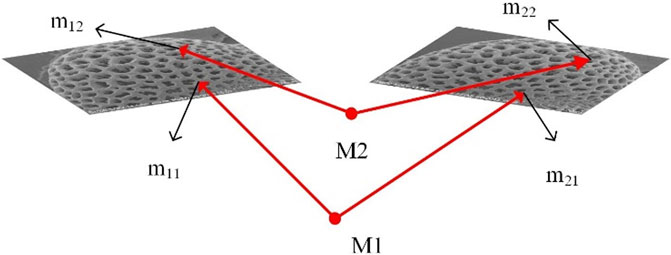
FIGURE 6. Simultaneous imaging equation of multiple image points.

The feature point m₁₁ can be detected on the first SEM image, Set M₁ as m₁₁ corresponding to the world point, the X and Y components of the world point M₁ can be calculated using equation 3, set as X_M1 and Y_M1. Then, on the second SEM image, find the feature point m₂₁ that matches m₁₁. The world point corresponding to m₂₁ is M₁, and the equation for projecting the world point M₁ onto m₂₁ is as follows

$\left[\begin{array}{c}{u}_{m21}\\ v_{m21}\\ 1\end{array}\right]=\left[\begin{array}{ccc}a& 0& 0\\ 0& a& 0\\ 0& 0& 1\end{array}\right]\left[\begin{array}{cc}\begin{array}{cc}\begin{array}{c}{r}_{11}\\ r_{21}\\ 0\end{array}& \begin{array}{c}{r}_{12}\\ r_{22}\\ 0\end{array}\end{array}& \begin{array}{cc}\begin{array}{c}{r}_{13}\\ r_{23}\\ 0\end{array}& \begin{array}{c}{t}_x\\ t_y\\ 1\end{array}\end{array}\end{array}\right]\left[\begin{array}{c}\begin{array}{c}{\mathrm{X}}_{M1}\\ {\mathrm{Y}}_{M1}\end{array}\\ \begin{array}{c}{\mathrm{Z}}_{M1}\\ 1\end{array}\end{array}\right],(4)$

In equation (4), a, X_M1, Y_M1 are known quantities. As already introduced in section 2, rotating a certain angle around the Y-axis of the sample stage itself to obtain the next image, θ it can be used to calculate the rotation parameter r_ii, so r_ii is a known quantity. Now, there are three unknown variables t_x, t_y, and Z_M1 in Eq. (4), but there are only two equations. If a pair of identical image points m₁₂ and m₂₂ are added to two SEM images, there are world points M₂ corresponding to it. The X and Y components of M₂ are set to X_M2 and Y_M2, and the equation for projecting the world point M₂ to the image point m₂₂ is as follows:

$\left[\begin{array}{c}{u}_{m22}\\ v_{m22}\\ 1\end{array}\right]=\left[\begin{array}{ccc}a& 0& 0\\ 0& a& 0\\ 0& 0& 1\end{array}\right]\left[\begin{array}{cc}\begin{array}{cc}\begin{array}{c}{r}_{11}\\ r_{21}\\ 0\end{array}& \begin{array}{c}{r}_{12}\\ r_{22}\\ 0\end{array}\end{array}& \begin{array}{cc}\begin{array}{c}{r}_{13}\\ r_{23}\\ 0\end{array}& \begin{array}{c}{t}_x\\ t_y\\ 1\end{array}\end{array}\end{array}\right]\left[\begin{array}{c}\begin{array}{c}{\mathrm{X}}_{M2}\\ {\mathrm{Y}}_{M2}\end{array}\\ \begin{array}{c}{\mathrm{Z}}_{M2}\\ 1\end{array}\end{array}\right],(5)$

In equation 5, there are three unknowns: t_x, t_y, and Z_M2. Observing Equations 4, 5, it can be seen that t_x and t_y are fixed unknowns. For each increase in world point, the unknowns increase by one, which is the Z component of the world point. However, the number of equations increases by two. Assuming that n pairs of identical image points are detected on two SEM images, there are 2 * n equations with n+2 unknowns. When 2 * n > n+2, which is n ≥ 2, the equation is solvable. The above equation system can be simplified to the form of Ax = b. There are many methods to solve this type of equation, and experiment in this article uses the generalized inverse of the matrix to solve it. In this way, a series of three-dimensional coordinates of the world points are obtained, as well as the relative translational motion t_x and t_y between the two SEM images. At this point, the external motion parameters between the two SEM images are known.

3.3 Triangulation

Section 3.2 provides the solution process for the Z component of the world point, t_x and t_y. Combining the X and Y components described in Eq. (3), the three-dimensional coordinates of the world point can be formed. However, in a large number of matching image points, there may be incorrect matches. If incorrect matches are included in the equation set, it will contaminate the equation set and affect the accuracy of solving other unknown quantities. Therefore, after estimating t_x and t_y, we still use triangulation to restore the point clouds, even if there are incorrect matches, it will not affect the solution of other points. After obtaining the internal and external motion parameters of two SEM images, the projection matrix can be calculated, and combined with a series of corresponding image points, the point clouds can be obtained through triangulation. The formula is as follows

$\left[\begin{array}{c}{u}_i\\ v_i\\ 1\end{array}\right]=P\left[\begin{array}{c}\begin{array}{c}X\\ Y\end{array}\\ \begin{array}{c}Z\\ 1\end{array}\end{array}\right]withi=\mathrm{1,2},(6)$

In equation (6), P is the projection matrix, which is composed of the SEM internal and external parameter matrices in equation 5. For a set of identical image points, there are four equations, and the coordinates of the corresponding world point have three unknown quantities. The method for solving the equation system composed of equation 6 is already a mature theory and will not be repeated.

4 Experimental process and results

4.1 Experimental data and process

Table 1 shows the detailed data of the 3D SEM image set, a in Table 1 is obtained by dpi and scale.

TABLE 1

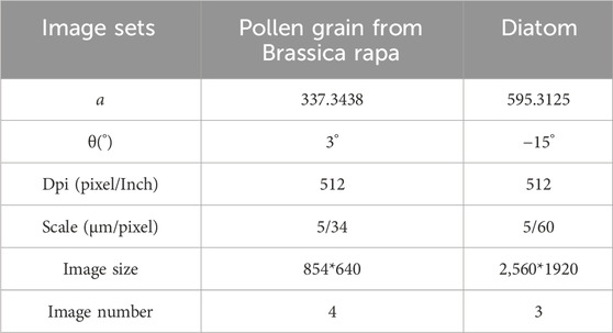
TABLE 1. Detailed parameters of the 3D SEM image set.

This experiment was implemented on Matlab 2020a, where the point clouds registration used the pcregistericp function, the input parameters of this function are fixed asfollows pcregistericp (ptCloud2,ptCloud1,’MaxIterations’,10,000,'Tolerance’, [1e-5,1e-3]), and the specific process is as follows:

1) The SEM sample stage rotates continuously around its Y-axis at a fixed angle to obtain a sequence of SEM images.

2) In the SEM image sequence, two adjacent images are grouped together, and feature detection and matching are performed on each group of images.

3) Within a set of images, according to equation 3, the X and Y components of the world point corresponding to the matching image points are calculated using the feature points detected on the previous image.

4) Within a set of images, according to the formula in section 3.2, the relative translation vector between the two images is estimated by imaging equation system of points on the latter image

5) For multiple sets of images, triangulation is performed to calculate the point clouds sequence. It should be noted that relative rotation and relative translation are used to calculate the projection matrix within the each set of images, resulting in a rotational motion difference between the point clouds sequences, which will provide a true rotation matrix for the evaluation criteria of relative rotation error in point clouds registration. In fact, for image sequences, if a global rotation matrix can be used, and the translation vector is still a relative translation vector, the estimated rotation transformation matrix between point clouds sequence is the third-order identity matrix.

6) Point clouds registration.

4.2 Experimental results

The implementation of our method for the two examples in Table 1 is shown in Figure 7 to Figure 8, which show the original SEM image a), the obtained point clouds b), and the meshed surface c).

FIGURE 7

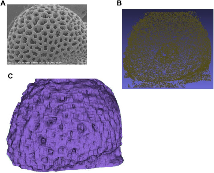
FIGURE 7. Example of Pollen reconstruction results. (A) SEM image, (B) Point clouds, (C) Surface mesh.

FIGURE 8

FIGURE 8. Example of Diatom reconstruction results. (A) SEM image, (B) Point clouds, (C) Surface mesh.

5 Comparison and analysis

5.1 Point clouds registration evaluation criteria

5.1.1 Root mean square error

Root mean square error (RMSE) is the average Euclidean distance between the nearest neighboring points of two point clouds after registration. The smaller the error, the closer the two point clouds align. The RMSE calculation formula is shown in Eq. (7). For multiple point clouds registration, this article adopts multiple RMSEs to calculate the average.

$RMSE=\sqrt{\frac{{\displaystyle \sum _i^n}{d}_i^2}{n}}$

$di=\sqrt{{\left(x_p-x_q\right)}^2+{\left(y_p-y_q\right)}^2+{\left(z_p-z_q\right)}^2,}(7)$

5.1.2 Relative rotation error

Relative rotation error (RRE) is a comparison between the rotation matrix obtained from registration results and the existing true rotation transformation matrix. The RRE calculation formula is shown in Eq. (8), where Re is the true rotation transformation matrix, and Rc⁻¹ is the inverse of the relative rotation matrix obtained from point clouds registration. The closer the RRE is to 0, the closer the estimated rotation is to the true rotation. For multiple point clouds registration, this article adopts multiple RREs to calculate the average.

$RRE=\arccos \left(\frac{trace\left(R_e{R}_c^{-1}\right)-1}{2}\right)\ast \frac{180}{\pi },(8)$

The method for the control experiment is the one proposed by (Rehman, 2018), which is also based on generating multiple point clouds from multiple adjacent image pairs and then registering them. The difference is that Rehman used disparity depth mapping to generate point clouds, while this article obtain multiple point clouds by estimating motion parameters then triangulates. In order to ensure the objectivity of the results, the point clouds size of the two experiments was scaled to the size of the real sample. The parameters of the point clouds registration function pcregistericp in both experiments, such as the number of iterations and step accuracy, were consistent. Then compare the root mean square error (RMSE) and relative rotation error (RRE) of point clouds registration. After running the program 20 times, the results are shown in Figure 9 to Figure 10. Figure 11 to Figure 12 show the mean values of RMSE and RRE after 20 runs, Table 2 shows the standard deviation of the result data.

FIGURE 9

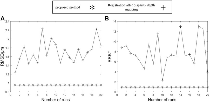
FIGURE 9. For example, pollen, RMSE (A) and RRE (B) curves after 20 runs.

FIGURE 10

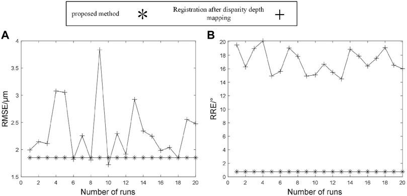
FIGURE 10. For example, diatom, RMSE (A) and RRE (B) curves after 20 runs.

FIGURE 11

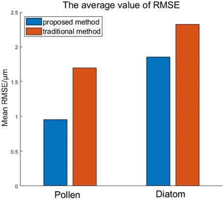
FIGURE 11. In two examples, the average value of the RMSE curve.

FIGURE 12

FIGURE 12. In two examples, the average value of the RRE curve.

TABLE 2

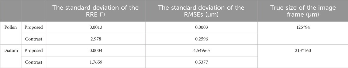
TABLE 2. Standard deviation of RMSE and RRE after 20 runs.

By observing Figure 9 to Figure 10, it can be seen that compared to traditional disparity depth mapping methods, the RMSE of the point clouds sequence generated by our method after registration is reduced in both examples, and RRE is significantly reduced in the diatom example. Furthermore, by analyzing Figures 11, 12, in the pollen example, the average RMSE reduction and RRE reduction are 44% and 88% by of our method, in the diatom example, the average RMSE decreased by 20% and the average RRE decreased by 96%. By observing Figures 9, 10, it can be found that after 20 runs, the results curves of RMSE and RRE of our method are very close to straight lines. Furthermore, from the standard deviation of the above data in Table 2, it can be seen that the standard deviation of our method after multiple runs is lower than that of traditional methods by multiple orders of magnitude, proving that our method has significant advantages in stability.

6 Disscussion and clusions

Although parallax depth mapping and SFM can also be applied on standard SEM devices, the point clouds registration method after parallax depth mapping requires the sample stage to perform a special rotation motion as shown in Figure 3A multiple times in a row, which limits the shooting angle of the SEM device and the point clouds registration error is large and unstable. However, the method proposed in this paper only requires one special rotation motion as shown in Figure 3A to obtain the initial point clouds, the rotation and translation parameters of subsequent images can be estimated using the PnP algorithm, so the shooting angle of subsequent images is arbitrary and unrestricted. At the same time, the method proposed in this paper is based on point clouds obtained through triangulation, which can exclude some error points and noise points through the indicator of reprojection error, which is an indicator that disparity depth mapping does not have.

The difference between this method and SFM lies in the approach of obtaining initial three-dimensional points. SFM uses singular value decomposition of the essential matrix to estimate the initial rotation and translation parameters, thereby obtaining a projection matrix to solve the three-dimensional points. The rotation and translation parameters of subsequent images are also estimated using the PnP algorithm. SFM does not require SEM equipment to perform special movements on Figure 3A, Unfortunately, on publicly available 3D SEM datasets, the rotation parameters estimated through the essential matrix are far from the actual rotation parameters, making it impossible to obtain good initial point clouds. Fortunately, SEM equipment is an indoor device that can control rotation motion. Compared to SFM estimated rotation parameters, using known rotation parameters is more stable. Therefore, the method proposed in this article only requires one special motion as shown in Figure 3A, after obtaining the real rotation parameters, the translation parameters can be estimated by constructing an equation system through the imaging model, and then the initial point clouds can be obtained through triangulation. The rotation and translation parameters of subsequent images can also be estimated using the PnP algorithm. In fact, the method proposed in this article is a compromise between disparity depth mapping and SFM. We believe that the proposed method can replace the disparity depth mapping and SFM.

Data availability statement

The original contributions presented in the study are included in the article/Supplementary Material, further inquiries can be directed to the corresponding author.

Author contributions

HD: Investigation, Methodology, Writing–original draft. HJ: Writing–review and editing, Data curation, Supervision. DQ: Conceptualization, Project administration, Writing–review and editing. DH: Funding acquisition, Project administration, Writing–review and editing.

Funding

The author(s) declare financial support was received for the research, authorship, and/or publication of this article. Project of Research on 3D Reconstruction Method of Ultrafine Microstructure Based on Scanning Electron Microscope Imaging (Z020026). This Project was supported by State Key Laboratory of Geomechanics and Geotechnical engineering.

Conflict of interest

The authors declare that the research was conducted in the absence of any commercial or financial relationships that could be construed as a potential conflict of interest.

Publisher’s note

All claims expressed in this article are solely those of the authors and do not necessarily represent those of their affiliated organizations, or those of the publisher, the editors and the reviewers. Any product that may be evaluated in this article, or claim that may be made by its manufacturer, is not guaranteed or endorsed by the publisher.

Supplementary material

The Supplementary Material for this article can be found online at: https://www.frontiersin.org/articles/10.3389/fenrg.2023.1333137/full#supplementary-material

References

Baghaie, A., Tafti, A. P., Owen, H. A., D’Souza, R. M., and Yu, Z. (2017). SD-SEM: sparse-dense correspondence for 3D reconstruction of microscopic samples. MICRON 97, 41–55. doi:10.1016/j.micron.2017.03.009

PubMed Abstract | CrossRef Full Text | Google Scholar

Basri, R., Jacobs, D. W., and Kemelmacher, I. (2007). Photometric stereo with general, unknown lighting. Int. J. Comput. Vis. 72 (3), 239–257. doi:10.1007/s11263-006-8815-7

CrossRef Full Text | Google Scholar

Bian, W. G. (2020). 3D imaging of dual secondary electron detectors in SEM. Suzhou: University of Suzhou of China, 43–56.

Google Scholar

Ding, W., Zhang, Y., Lu, H., Wan, W., and Shen, Y. (2019). Automatic 3D reconstruction of SEM images based on Nano-robotic manipulation and epipolar plane images. ULTRAMICROSCOPY 200, 149–159. doi:10.1016/j.ultramic.2019.02.014

PubMed Abstract | CrossRef Full Text | Google Scholar

Eulitz, M., and Reiss, G. (2015). 3D reconstruction of SEM images by use of optical photogrammetry software. J. Struct. Biol. 191 (2), 190–196. doi:10.1016/j.jsb.2015.06.010

PubMed Abstract | CrossRef Full Text | Google Scholar

Goldman, D. B., Curless, B., Hertzmann, A., and Seitz, S. M. (2010). Shape and spatially-varying brdfs from photometric stereo. IEEE Trans. Pattern Analysis Mach. Intell. 32 (6), 1060–1071. doi:10.1109/tpami.2009.102

PubMed Abstract | CrossRef Full Text | Google Scholar

Huang, L., Dontsov, E., Fu, H., Lei, Y., Weng, D., and Zhang, F. (2022). Hydraulic fracture height growth in layered rocks: perspective from DEM simulation of different propagation regimes. Int. J. Solids Struct. 238, 111395. doi:10.1016/j.ijsolstr.2021.111395

CrossRef Full Text | Google Scholar

Huang, L., He, R., Yang, Z., Tan, P., Chen, W., Li, X., et al. (2023b). Exploring hydraulic fracture behavior in glutenite formation with strong heterogeneity and variable lithology based on DEM simulation. Eng. Fract. Mech. 2023, 278, 109020.

CrossRef Full Text | Google Scholar

Huang, L., Liu, J., Zhang, F., Fu, H., Zhu, H., and Damjanac, B. (2020). 3D lattice modeling of hydraulic fracture initiation and near-wellbore propagation for different perforation models. J. Pet. Sci. Eng. 191, 107169. doi:10.1016/j.petrol.2020.107169

CrossRef Full Text | Google Scholar

Huang, L., Tan, J., Fu, H., Liu, J., Chen, X., Liao, X., et al. (2023a). The non-plane initiation and propagation mechanism of multiple hydraulic fractures in tight reservoirs considering stress shadow effects. Eng. Fract. Mech. 292, 109570. doi:10.1016/j.engfracmech.2023.109570

CrossRef Full Text | Google Scholar

Ikeuchi, K. (1981). Determining surface orientations of specular surfaces by using the photometric stereo method. IEEE Trans. Pattern Analysis Mach. Intell. 3 (6), 661–669. doi:10.1109/tpami.1981.4767167

PubMed Abstract | CrossRef Full Text | Google Scholar

Ji, Y., Wang, J., and Huang, L. (2015). Analysis on inflowing of the injecting Water in faulted formation. Adv. Mech. Eng. 7, 1–10. doi:10.1177/1687814015590294

CrossRef Full Text | Google Scholar

Kareiva, S., Selskis, A., Ivanauskas, F., Šakirzanovas, S., and Kareiva, A. (2015). Scanning electron microscopy: extrapolation of 3D data from SEM micrographs. MATER SCI-MEDZG 21 (4), 640–646. doi:10.5755/j01.ms.21.4.11101

CrossRef Full Text | Google Scholar

Li, M., Deng, S., Yan, P., et al. (2016). Research on the toughening mechanism of fiber/Whisker on oil well cement stone. J. Southwest Petroleum Univ. Sci. Technol. Ed. 38 (05), 151–156.

Google Scholar

Liu, Q., Li, J., Liang, B., et al. (2023). Complex wettability behavior triggering mechanism on imbibition: a model construction and comparative study based on analysis at multiple scales. Energy, 275, 127434. doi:10.1016/j.energy.2023.127434

CrossRef Full Text | Google Scholar

Liu, X. J. (2018). Visual computing based micro-nano scale 3D SEM topography measurement. Wuhan: Huazhong University of Science and Technology of China, 77–81.

Google Scholar

Luo, H., Xie, J., Huang, L., Wu, J., Shi, X., Bai, Y., et al. (2022). Multiscale sensitivity analysis of hydraulic fracturing parameters based on dimensionless analysis method. Lithosphere 2022, 9708300. doi:10.2113/2022/9708300

CrossRef Full Text | Google Scholar

Munawar, M. J., Lin, C., Chunmei, D., Zhang, X., Zhao, H., Xiao, S., et al. (2018a). Architecture and reservoir quality of low-permeable Eocene lacustrine turbidite sandstone from the Dongying Depression, East China. Open Geosci. 10 (1), 87–112. doi:10.1515/geo-2018-0008

CrossRef Full Text | Google Scholar

Munawar, M. J., Lin, C., Cnudde, V., Bultreys, T., Chunmei, D., Zhang, X., et al. (2018b). Petrographic characterization to build an accurate rock model using micro-CT: case study on low-permeable to tight turbidite sandstone from Eocene Shahejie Formation. Micron 109, 22–33. doi:10.1016/j.micron.2018.02.010

PubMed Abstract | CrossRef Full Text | Google Scholar

Munawar, M. J., Vega, S., Lin, C., Alsuwaidi, M., Ahsan, N., and Bhakta, R. R. (2021). Upscaling reservoir rock porosity by fractal dimension using three-dimensional micro-computed tomography and two-dimensional scanning electron microscope images. J. Energy Resour. Technol. 2021 (1), 143. doi:10.1115/1.4047589

CrossRef Full Text | Google Scholar

Rehman, W. (2018). 3D SEM surface reconstruction from multi-view images. Wisconsin: University of Wisconsin-Milwaukee of America. https://dc.uwm.edu/etd/1908.

Google Scholar

Reimer, L. (1985). Scanning electron microscopy:physics of image formation and microanalysis. Opt. Acta Int. J. Opt. 31 (8), 848. doi:10.1080/713821585

CrossRef Full Text | Google Scholar

Samak, D., Fischer, A., and Rittel, D. (2007). 3D reconstruction and visualization of microstructure surfaces from 2D images. CIRP Ann. - Manuf. Technol. 56 (1), 149–152. doi:10.1016/j.cirp.2007.05.036

CrossRef Full Text | Google Scholar

Song, R., Liu, J., and Cui, M. (2017). A new method to reconstruct structured mesh model from micro-computed tomography images of porous media and its application. Int. J. Heat Mass Transf. 109, 705–715. doi:10.1016/j.ijheatmasstransfer.2017.02.053

CrossRef Full Text | Google Scholar

Song, R., Wang, Y., Ishutov, S., Zambrano-Narvaez, G., Hodder, K. J., Chalaturnyk, R. J., et al. (2020). A comprehensive experimental study on mechanical behavior, microstructure and transport properties of 3D-printed rock analogs. Rock Mech. Rock Eng. 53, 5745–5765. doi:10.1007/s00603-020-02239-4

CrossRef Full Text | Google Scholar

Sutton, M. A., Li, N., Garcia, D., Cornille, N., Orteu, J. J., McNeill, S. R., et al. (2007). Scanning electron microscopy for quantitative small and large deformation measurements Part II: experimental validation for magnifications from 200 to 10,000. Exp. Mech. 47 (6), 789–804. doi:10.1007/s11340-007-9041-0

CrossRef Full Text | Google Scholar

Tafti, A. P., Holz, J. D., Baghaie, A., Owen, H. A., He, M. M., and Yu, Z. (2016). 3DSEM++: adaptive and intelligent 3D SEM surface reconstruction. MICRON 87, 33–45. doi:10.1016/j.micron.2016.05.004

PubMed Abstract | CrossRef Full Text | Google Scholar

Tafti, A. P., Kirkpatrick, A. B., Alavi, Z., Owen, H. A., and Yu, Z. (2015). Recent advances in 3D SEM surface reconstruction. MICRON 78, 54–66. doi:10.1016/j.micron.2015.07.005

PubMed Abstract | CrossRef Full Text | Google Scholar

Tan, P., Fu, S. H., Chen, Z. W., and Zhao, Q. (2023). Experimental investigation on fracture growth for integrated hydraulic fracturing in multiple gas bearing formations. Geoenergy Sci. Eng. 2023, 212316. doi:10.1016/j.geoen.2023.212316

CrossRef Full Text | Google Scholar

Tan, P., Pang, H., Zhang, R., Jin, Y., Zhou, Y., Kao, J., et al. (2020). Experimental investigation into hydraulic fracture geometry and proppant migration characteristics for southeastern Sichuan deep shale reservoirs. J. Pet. Sci. Eng. 184, 106517. doi:10.1016/j.petrol.2019.106517

CrossRef Full Text | Google Scholar

Wang, Q., Zhu, F., Sun, M., et al. (2013). Three-dimensional reconstruction techniques based on one single SEM image. Nami Jishu yu Jingmi Gongcheng/Nanotechnology Precis. Eng. 11 (6), 541–545.

Google Scholar

Wang, X. Q., Jin, X., Li, J. M., et al. (2019). FIB-SEM applications in petroleum geology research. J. Chin. Electron Microsc. Soc. 38 (3), 303–319. doi:10.3969/j.issn.1000-6281.2019.03.015

CrossRef Full Text | Google Scholar

Wu, M., Jiang, C., Song, R., et al. (2023). Comparative study on hydraulic fracturing using different discrete fracture network modeling: insight from homogeneous to heterogeneity reservoirs. Eng. Fract. Mech., 284, 109274. doi:10.1016/j.engfracmech.2023.109274

CrossRef Full Text | Google Scholar

Yao, S. X., Cheng, H. R., Xiong, Z., et al. (2022). Method characterizing shale oil reservoirs in Jimsar based on quantitative digital analysis of cuttings. OIL Drill. Prod. Technol. 44 (01), 117–122.

Google Scholar

Yi, J., Ma, S. J., Zhong, K., et al. (2019). A locally efficient 3D measurement method under SEM. Transducer Microsyst. Technol. 38 (11), 133–135.

Google Scholar

Zhang, C. M., Guo, X. Y., and Cheng, X. W. (2013). Study on the interface characteristics of N80 steels and silica matrix coatings and well cement. J. Southwest Petroleum Univ. Sci. Technol. Ed. 35 (01), 144–149. doi:10.3863/j.issn.1674-5086.2013.01.022

CrossRef Full Text | Google Scholar

Zhang, Z. Y. (1996). A new multistage approach to motion and structure estimation:from essential parameters to euclidean motion via fundamental matrix. France: INRIA Sophia-Antipolist.

Google Scholar

Zhu, Z. B. (2013). Fractal features research on the microscopic pore structure of petroleum reservoir rocks. Heilongjiang: Northeast Petroleum University of China, 11–18.

Google Scholar