 Minghu Wang
 Yushuo Xia
 Xinsheng Zhang
- School of Management, Xi’an University of Architecture and Technology, Xi’an, China
This paper introduces a novel coupling method to enhance the precision of short- and medium-term renewable energy power load demand forecasting. Firstly, the Tent chaotic mapping incorporates the standard WOA and modifies its internal convergence factor to a nonlinear convergence mode, resulting in an improved IWOA. It is used for the weight optimization part of BILSTM. Then, the SA is introduced to optimize the learning rate, the number of nodes in hidden layers 1 and 2, and the number of iterations of BILSTM, constructing an IWOA-SA-BILSTM prediction model. Finally, through case analysis, the prediction model proposed in this paper has the highest improvement of 76.7%, 74.5%, and 45.9% in terms of Mean Absolute Error, Root Mean Square Error, and R2, respectively, compared to other optimal benchmark models, proving the effectiveness of the model.
1 Introduction
In order to accelerate the transformation of the industrial structure of the power system, China has vigorously promoted the development of renewable energy power, and in recent years more and more renewable energy power has been incorporated into the power grid system. With the increase in installed capacity of renewable energy power generation, the planning and deployment of power has gradually become the focus of the grid work system. The power sector’s production deployment and optimal planning depends on the accuracy of power demand forecasting, therefore, improve the accuracy of renewable energy power demand forecasting is the focus of the current power workers research.
The process of forecasting electricity can be divided into three stages: ultra-short-term forecasting, short-term forecasting, and medium-and long-term forecasting. Ultra-short-term forecasting is to forecast the future power load demand in terms of hours; short-term forecasting is to forecast the power load demand in the future period in terms of days, weeks, and quarters; and medium- and long-term forecasting is to forecast the power load demand in the future time in terms of years. Currently, short-term forecasting has become the focus of renewable energy power demand research.
Researchers worldwide are conducting studies to enhance the accuracy of forecasting electricity demand. Forecasting methods are primarily divided into three categories: statistical, artificial intelligence, and hybrid. Statistical methods mainly include time series forecasting models (Dong, 2019; Ma et al., 2022; Gao, 2023) and exponential smoothing models (Trull et al., 2021). For example, Shang Fangyi et al. (Shang et al., 2015) utilized the gray Verhulst model to enhance the precision of electricity demand analysis and forecasting; Zhang Tao et al. (Zhang and Gu, 2018) introduced Markov chains into the study of renewable energy load forecasting, and achieved effective results; Luo Yi-wang (Luo, 2018) applied the ARMR model to the study of electricity demand forecasting methods, and claimed that the forecasting errors were less than 1% in all of their studies; Zhang Yunfei et al. (Zhang Yunfei et al., 2021) developed a grid peaking demand forecasting model using ridge regression, demonstrating its effectiveness through a case study; Wu et al. (He et al., 2021) combined the Seasonal Exponential Adjustment Method (SEAM) with the time series regression method for the study of load demand forecasting and confirmed the superiority of the model. Artificial intelligence forecasting methods include Extreme Learning Machine (ELM) (He et al., 2021), Support Vector Machine (SVM) (Shi et al., 2019; MuSAA et al., 2021), and various neural network forecasting models (Machado et al., 2021; Rajbhandari et al., 2021; Hu et al., 2023). For example, Shi et al. (Shi et al., 2012) utilized SVM to forecast the amount of photovoltaic (PV) load generation and claimed that the results were good; Zare-Noghabi et al. (Zare-Noghabi et al., 2019) demonstrated the effectiveness of Support Vector Regression (SVR) in forecasting power system load demand using actual data; Guo et al. (Guo et al., 2021) developed a load forecasting model using LSTM, considering demand response, and demonstrated its practicality through experiments; Wen et al. (Wen et al., 2022) proposed a short-term load demand forecasting model based on Bi-directional Long Short-Term Memory(BILSTM) considering the uncertainty of short-term load demand and claimed that the model was superior to the traditional forecasting methods; Su Chang et al. (Su et al., 2023) utilized LSTM and combined it with multi-feature fusion coding to forecast the power load demand, which improved the accuracy of the power load forecasting; Zhang Suning et al. (Zhang et al., 2022) proposed a cross-region power demand forecasting model based on XGBoost for different forms of power demand in multiple regions and claimed that the method can provide fast and accurate forecasting of power demand; Shu Zhang et al. (Zhang Shu et al., 2021) proposed a neural network forecasting model based on feature analysis of the LSTM, which improves the prediction accuracy of short-term power demand. Hybrid forecasting methods (Qinghe et al., 2022; He et al., 2023; Sekhar and Dahiya, 2023) combine various effective forecasting methods to enhance the accuracy of electricity demand forecasting. For example, Moalem et al. (Moalem et al., 2022) successfully combined the ELATLBO method with LSTM neural network for power demand forecasting through experiments; Hu et al. (Hu et al., 2019) proposed a decomposition-based combined forecasting model, which will have the advantage of being able to dynamically combine various models based on data.
At present, more and more scholars have started using ensemble models to improve the accuracy and effectiveness of renewable energy demand prediction research. Various optimization algorithms have also been used by many scholars to optimize the parameters of basic prediction models, thereby further improving the prediction performance of the models. Simulated Annealing Algorithm (SAA) and Whale Optimization Algorithm (WOA) are two optimization algorithms with good performance. SAA has the following advantages: 1. The algorithm boasts a superior global optimization ability, enabling it to find the global optimal solution, thereby avoiding local optimal solutions; 2. SAA is suitable for dealing with large-scale complex problems; 3. Compared with other algorithms, SAA has simpler description, more flexible use, higher operating efficiency, and is less affected by initial conditions; 4. SA does not depend on the specific form and attributes of the problem, only needs to define the objective function and neighbor structure. WOA has the following advantages: 1. Simulating natural behavior makes it have stronger optimization ability; 2. The three population update mechanisms of WOA are independent of each other, and the global search and local development processes can be separately run and controlled, which is beneficial to find the optimal solution; 3. WOA does not require manual setting of various parameters, reducing the difficulty of use and improving the operation efficiency; 4. WOA has shown good optimization performance in solving many numerical optimization and engineering problems. Therefore, this article chooses two optimization algorithms to enhance the prediction accuracy and effectiveness of the basic algorithm.
Therefore, this article adopts a bidirectional long short-term memory network (BILSTM) as the benchmark prediction model. Firstly, the benchmark whale optimization algorithm (WOA) has been improved by incorporating Tent chaos mapping and nonlinear convergence factor to create an evolutionary whale optimization algorithm (IWOA); then the weight matrix of BILSTM is optimized using the evolutionary whale optimization algorithm (IWOA); at the same time, the simulated annealing algorithm (SA) is utilized simultaneously to optimize crucial parameters of BILSTM. Finally, the effectiveness and feasibility of the proposed model are verified using real-world data from a region in China.
The contributions of this article can be summarized as follows: 1. A new coupling algorithm is proposed to predict the demand for renewable energy power, which enhances the accuracy and efficiency of prediction. 2. The standard WOA algorithm has been enhanced to improve its global search and local optimization capabilities, potentially paving the way for future research. 3. The BILSTM model’s prediction performance is enhanced by introducing a heuristic algorithm to optimize its weights and key parameters.
2 Factor analysis and data processing
2.1 Renewable electricity demand analysis
There are many factors that affect the demand for renewable electricity, which can be categorized into significant and non-significant factors. Significant factors, i.e., factors that can cause large fluctuations in the demand for renewable electricity within a short period of time, are mainly meteorological factors, such as temperature, humidity, atmospheric pressure, and so on. Secondly, the power generation of fossil energy will also have an impact on the demand for renewable electricity, because if fossil energy cannot support the general demand for electricity by residents within a short period of time, then the social electricity consumption needs to be supported by renewable electricity, so the power generation of fossil energy is taken as a significance factor. Fossil power generation is also considered as a significant factor, as the fluctuation in electricity demand during legal holidays can also be caused by short periods of time. Non-significant factors, i.e., factors that require a long period of sustained influence to cause fluctuations in renewable energy power demand, generally include economic factors, policy factors, etc. As this paper aims to improve the accuracy of short-term demand forecasting of renewable electricity, the non-significant factors are considered to be stable in this study, and the significant factors are emphasized for in-depth study.
2.2 Factor data analysis
Meteorological data includes three types of factors, namely, temperature, relative humidity and atmospheric pressure, with the temperature factor divided into maximum, minimum and average temperatures. According to the existing data statistics, when the daily relative humidity is higher than 80%, the demand for electricity will rise, while when the daily relative humidity is lower than 51%, the demand for electricity will be relatively low, so this paper takes the relative humidity as one of the influencing factors. Secondly, according to the existing data, holidays and legal holidays also cause large fluctuations in peak electricity consumption, so holidays are also an influential factor that cannot be ignored in the study of renewable electricity demand. In this study, the sum of the number of days of holidays and legal holidays is used as the value of the holiday indicator.
Since the scope of this paper is the renewable energy power demand within the province, the temperature indicator takes the average temperature as the temperature state of the province. The provincial average temperature is weighted and averaged with the temperature values of the municipalities in the province to obtain the final provincial average temperature. Let the average temperature of the province as
Among them,
This paper uses Pearson correlation coefficient to verify the correlation between temperature data and renewable energy power load demand data in historical data to enhance experimental data validity and scientificity:
The test results are shown in Table 1, the correlation coefficients between all three types of temperature indicators and renewable energy power load demand are greater than 0.3, indicating that all three types of temperature indicators have a non-negligible impact on renewable energy power load demand, and therefore all three types of temperatures will be used as research factors.
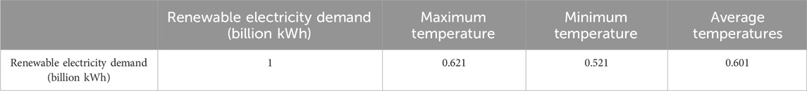
TABLE 1. Pearson’s coefficients for renewable energy load demand and various types of temperatures.
In addition, there may be linear correlation between various types of factors, which leads to the emergence of multicollinearity problem and affects the prediction accuracy of the model. Therefore, this paper does the covariance test using variance inflation factor (VIF) on the collected data, and eliminates the covariance between the influencing factors through LASSO regression, and finally utilizes the filtered data for renewable energy power load demand prediction. The formula for variance inflation factor (VIF) is as follows:
Where
3 Multidimensional feature analysis and prediction model based on IWOA-SAA-BILSTM
This part constructs the IWOA-SAA-BILSTM prediction model. There are three steps in the construction process: 1. Building and improving the standard Whale Optimization Algorithm (WOA), introducing the Tent chaotic mapping algorithm to enhance WOA’s global solution-seeking ability in the solution process and avoid it easily falling into local optimal solutions. At the same time, the convergence factor in WOA is improved to be nonlinear, which can better simulate the predation mechanism of whale populations and improve the algorithm’s global search ability. 2. The BILSTM model’s prediction effect is enhanced by optimizing the weights using the improved Whale Optimization Algorithm (IWOA). 3. Introducing simulated annealing algorithm (SAA) to optimize four hyperparameters of BILSTM’s hidden layer 1 and hidden layer 2, including the number of neurons, iteration rate, and learning rate. After the above three steps, the IWOA-SAA-BILSTM prediction model is constructed.
3.1 Whale optimization algorithm and its improvement
3.1.1 Whale optimization algorithm
The Whale optimization algorithm, introduced by Australian scholars Mirjalili et al., in 2016, is an intelligent optimization method. The idea of this algorithm originates from the hunting behavior of humpback whales, which have two main hunting behaviors, the first one is encircling hunting and the other one is bubble net hunting. In this algorithm, the position of each individual whale during the hunting process is considered as a potential solution to the problem to be optimized (Yin et al., 2023). The algorithm uses a random search agent and a spiral structure to simulate the humpback whale bubble net attack mechanism, offering a simple optimization search mechanism and local optimum jump capability.
3.1.1.1 Surrounding the prey
The WOA algorithm is a method used to optimize the global solution space of a problem when a group of whales hunt for prey. The target prey is considered the optimal solution, and the current location searched by a whale is considered the best candidate solution. When the best candidate solution is defined, other whales flock to it, and Equation 4 represents the distance between other whales and the best candidate solution:
where
Equation 5 is the formula for updating the position of an individual whale during the t+first search:
Where
3.1.1.2 Bubble net hunting
Humpback whales use contraction encirclement and spiral renewal predation methods in bubble nets, choosing based on the probability of the mechanism, p, within the [0,1] range. When p < 0.5, humpback whales choose the contraction encirclement method; when p ≥ 0.5, humpback whales use the spiral renewal mechanism.
When contraction envelopment is used, the distance between individual whales is reduced by a convergence factor
When the spiral update mechanism is used, the position update between it and the target prey uses the spiral update mechanism with the following expression:
Style:
3.1.1.3 Random search for prey
When
Style:
3.1.2 Improved whale optimization algorithm
The optimization ability of a swarm intelligence algorithm is influenced by the diversity and uniformity of its initialization population. The traditional whale optimization algorithm adopts random number to generate the initial population, which leads to the uneven distribution of the initial population and too much simplicity. In the process of population optimization, it cannot optimize in the whole solution space, which leads to some solution sets cannot be found, and ultimately leads to the algorithm falling into the local optimal state. At the same time, it will also affect the convergence speed of the algorithm. Tent chaotic mapping can generate chaotic sequences with strong randomness, universality and uniformity, which can improve the problem that WOA falls into local optimal in the process of population iteration. At the same time, the standard WOA algorithm’s convergence factor decreases linearly with population iterations until it reaches 0, adjusting global search and local development abilities of the population. However, the article introduces a nonlinear convergence factor to the standard WOA algorithm, which enhances its capacity to simulate population predation and optimize population optimization, as the linear decrease of convergence factor a cannot effectively adjust global search ability and local development ability.
3.1.2.1 Tent chaos mapping initialization population
Tent chaotic mapping maps the optimization variables to the value intervals of the entire solution space through the chaotic mapping rules, so as to make use of the universality, uniformity and regularity of the chaotic variables for optimization, and ultimately transform the optimization solution set into the optimization space. Tent chaotic mapping is characterized by a uniform distribution of the functions and good correlation between the functions, and its expression is as follows:
where
The WOA after adding chaotic mapping is able to produce a uniformly distributed initial population during the process of population initialization, thus avoiding the defect of the algorithm falling into local optimum. Figures 1, 2 show the distribution of the initial population before and after the addition of the Tent chaotic mapping.
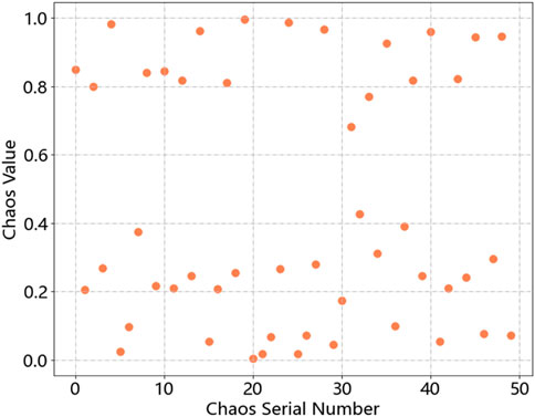
FIGURE 1. Population distribution after adding Tent chaotic mapping.
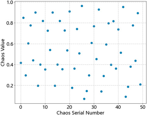
FIGURE 2. Population distribution before adding Tent chaotic mapping.
3.1.2.2 Nonlinear convergence factor
The improved convergence factor is used to vary the factor size in a nonlinear way with the following update formula:
where
The flowchart of the improved whale optimization algorithm is shown in Figure 3.
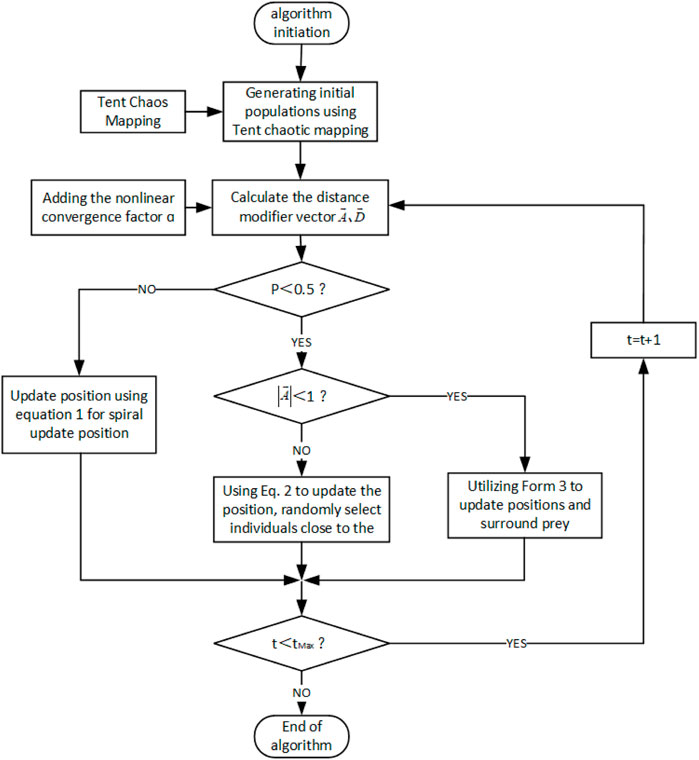
FIGURE 3. Flowchart of IWOA algorithm.
The specific steps are:
1. Introduce Tent chaotic mapping, use Tent chaotic mapping to initialize the population, set the maximum number of iterations of the population
2. Calculate the fitness of individual whales in the population, confirm the optimal whale individual in the current population and keep its position information;
3. Add a nonlinear convergence factor
4. Make a judgment on the mode
5. After the position update of the population, calculate the fitness of each whale individual in the population again, compare it with the fitness of the previous optimal whale individual, and if it is better than that, replace the previous optimal whale individual with the current whale individual;
6. Determine whether the population reaches the maximum number of iterations, if so, output the optimal solution, otherwise return to step 3 for the next iteration.
3.2 Simulated annealing algorithm
The Simulated Annealing Algorithm (SAA) is a stochastic optimization technique developed in the early 1980s, employing the Monte Carlo iterative solution strategy. The algorithm simulates the physical process in thermodynamics in which an object gradually cools down from some higher temperature and is called annealing. The advantage of the simulated annealing algorithm is its ability to select the worse of the solutions in the current solution neighborhood with a certain probability, which avoids the problem of local optimality and thus achieves the advantage of finding the optimal solution globally.
The main step of the Simulated Annealing Algorithm consists of two inner and outer loops. The outer loop defines the algorithm loop’s termination condition, while the inner loop focuses on finding a new optimal solution within the current hyperparameters of the bi-directional neural network. When the loop ends, the algorithm converges to the optimal solution. The specific steps are as follows:
1. Initialization parameters, set the cooling table temperature
2. Start the kth iteration at the current temperature,
3. Randomly generate a new solution
4. Compute the function
5. Determine the excellence of the solution. If
6. Slowly cool down the temperature, so that
3.3 Bidirectional long and short-term memory networks
The creation of BILSTM goes back to RNNs (Recurrent Neural Networks). RNNs are commonly utilized in time series prediction, but they often face issues like gradient vanishing or explosion when dealing with long time series, which leads to the algorithms failing to capture the long term dependencies. To solve this problem, researchers proposed LSTM (Long Short-Term Memory Neural Network). When the data is input to the LSTM, it selects the input value by adjusting the input gate parameter; the role of the forgetting gate when the extracted invalid information is eliminated, and at the same time, the extracted valid information will be input to the next mitigation, and finally, its structure is shown in Figure 4.
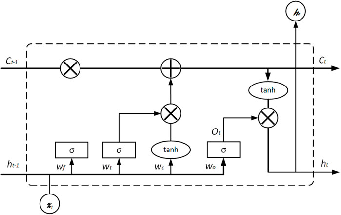
FIGURE 4. Structure of LSTM neural network.
However, with the widespread application of LSTM, researchers have found that LSTM has a problem of unidirectional prediction, which can only predict based on the forward information input to the neural network. To solve the unidirectional prediction problem of LSTM, BILSTM was born. BILSTM is composed of a forward LSTM and a backward LSTM under the same time series. Its gate unit is the same as that of standard LSTM, and its advantage is that it can combine forward and backward information to process input data bi-directionally, thus mining hidden features in the data sequence and improving the prediction effect. Its structure is shown in Figure 5.
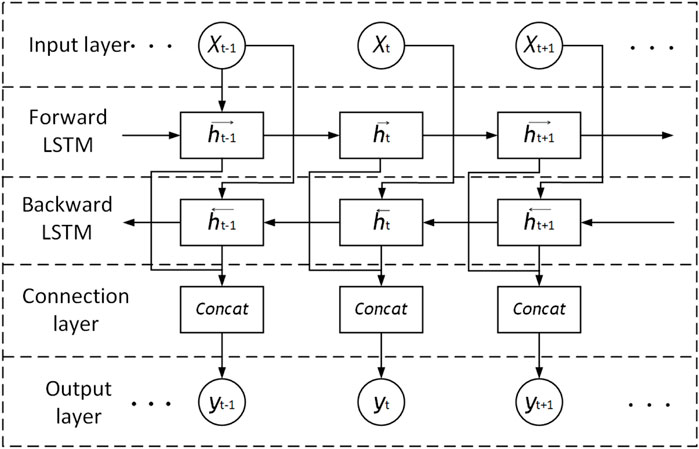
FIGURE 5. Structure of BILSTM neural network.
3.4 IWOA-SAA-BILSTM
In this paper, in order to improve the prediction effect of the benchmark BILSTM, the standard BILSTM algorithm is improved, which is mainly optimized for the weights and hyperparameters. Specifically, the improved whale optimization algorithm (IWOA) and simulated annealing algorithm (SAA) are introduced to optimize the weights and hyperparameters of BILSTM, respectively. The specific improvement ideas of the model are as follows: Firstly, tent chaos mapping is introduced as a new feature in the standard whale optimization algorithm (WOA)., so that the WOA can produce uniformly distributed populations to avoid falling into local optimum; then, the WOA’s convergence factor is modified to a nonlinear factor during iteration to enhance the optimality-seeking capacity of whale populations, and the improved IWOA is obtained; and the weights and hyperparameters of the standard BILSTM are optimized by using the IWOA. weights for optimization. At the SAA me time, the simulated annealing algorithm (SAA) is introduced to optimize the hyperparameters of the standard BILSTM, specifically including the number of nodes in the hidden layer 1, the number of nodes in the hidden layer 2, the number of neural network iterations, and the neural network learning rate. Finally, the IWOA-SAA-BILSTM prediction model is obtained. The flowchart of the algorithm is shown in Figure 6.
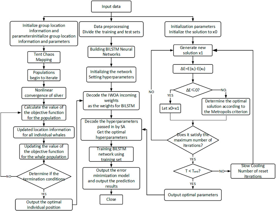
FIGURE 6. Flowchart of IWOA-SAA-BILSTM algorithm.
The specific steps of IWOA-SAA-BILSTM include:
1. Input data. Test the data for missing values and outliers and normalize the data. Divide the data, divide the training set and test set according to 4:1.
2. Construct the BILSTM network, initialize the parameters, set the number of hidden layer 1, the number of hidden layer 2, the learning rate, and the number of iterations.
3. Build the IWOA weight optimization model. Set the important parameters such as whale population size, number of population iterations, and spatial dimension; meanwhile, introduce Tent chaotic mapping to generate the initial whale population, and the other population converges and iterates according to the nonlinear way, and the objective function is to determine the value of the population. The optimal whale population position information is mapped into the weights of BILSTM.
4. Build the SAA optimization algorithm. Initialize the SAA parameters, set the cooling table temperature
5. Run the algorithm and judge whether IWOA and SAA reach the maximum number of iterations and whether it meets the termination conditions, respectively; if the weak algorithm meets the termination conditions, the optimal parameters are encoded and outputted to the BILSTM network, otherwise, repeat step 3.
6. After many iterations, the objective function with the minimum error as well as the optimal parameters and weights can finally be obtained, and finally the IWOA-SAA-BILSTM prediction model is obtained.
This article presents a model with several advantages:
a. The IWOA-SAA-BILSTM model improves the initial population distribution of the standard WOA by making it more uniform, the goal is to enhance the diversity of the population and enhance their global search ability. The introduction of a dynamic step factor enhances the optimization performance of the whale algorithm by regulating its local development and global search abilities.
b. The BILSTM network in the IWOA-SAA-BILSTM model has its own dual memory units and gating mechanism, which can effectively capture and store long-term dependencies in bidirectional sequences, and learn models and features from the data, which enables the model to better predict. In addition, the IWOA-SAA-BILSTM model optimizes the weights and important parameters of the BILSTM model to better leverage the predictive performance of BILSTM and improve prediction efficiency.
3.5 Pseudo code of main functions of the algorithm
1.Improve the whale optimization algorithm
def tent_map(x):
return 1–2 * abs(x)
#dynamic step factor
def dynamic_step_size(iter_num, max_iter, step_size)
return step_size/(iter_num/max_iter)
# Initialize whale optimization algorithm
whale_optimizer = initialize_whale_optimizer()
2.Simulated annealing algorithm initialization
simulated_annealing = initialize_simulated_annealing()
3.Initialize BILSTM neural network
bilstm_model = initialize_bilstm_model()
4.Constructing IWOA-SA-BILSTM
for iter_num in range(max_iter):
# Improving whale optimization algorithm using Tent chaotic mapping
whale_optimizer.improve(tent_map(whale_optimizer.position))
# Optimizing BILSTM weights using an improved whale optimization algorithm
bilstm_model.optimize(whale_optimizer.position)
# Optimizing BILSTM hyperparameters using simulated annealing algorithm
simulated_annealing.optimize(bilstm_model.hyperparameters)
# Dynamically adjust the step factor
whale_optimizer.step_size = dynamic_step_size(iter_num, max_iter, whale_optimizer.step_size)
4 Arithmetic analysis
4.1 Description of the arithmetic example
In this part, the renewable energy power load demand forecasting model IWOA-SAA-BILSTM proposed in this paper is used, for example, prediction to verify its reliability and superiority in practical application. The experimental data are taken from the official website of the National Bureau of Statistics of China, the China Price Information Network, and the Xihe Energy Big Data Platform, and the preliminary data are firstly extracted, and then the data are precisely analyzed according to the data processing method in the second part of this paper, and the data are collated to obtain a total of 72 monthly renewable energy power load demand and various types of data in Shaanxi Province of China, including the data of the renewable energy power load demand for the period from January 2017 to December 2022, including thermal power generation and the data of the renewable energy power load demand in China. The data reveals six influencing factors, including thermal power generation, maximum temperature, minimum temperature, average temperature, relative humidity, and the number of legal holidays, the dependent variable is the renewable energy power load demand, Figure 7 shows the change curve graph of load demand between January 2017 and December 2022.
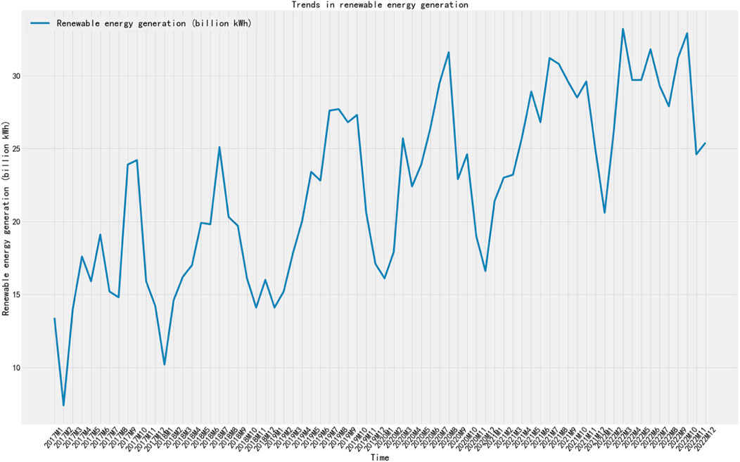
FIGURE 7. Renewable electricity load demand, January 2017 to December 2022.
4.2 Experimental environment and parameter settings
This article conducted experiments in a virtual Python3.9 environment on Anaconda2.0.3, using a Windows11 system laptop with an Intel Core i7-9750H CPU, NVIDIA GTX 1660ti GPU, and 16G RAM.
In existing research, it is known that among the hyperparameters of BILSTM neural networks, The number of hidden layer neurons (m) and learning rate (l) significantly influence the prediction performance of neural networks. The number of hidden layer neurons m in neural networks is usually determined by empirical formulas, as shown in formula (12). Using this formula, an approximate range of values for the number of hidden layer neurons in a neural network can be obtained. Within this range, specific parameter settings can be obtained through repeated experiments.
The formula involves α representing the number of output layer nodes, β representing the number of input layer nodes, and n being a constant.
The study employs the Adam optimizer with an initial learning rate of [0.0001, 0.01], a maximum of 500 iterations, and an initial population generated by Tent chaos; SA’s initial temperature is set to 100°C, and temperature decay frequency is set to 0.95; both IWOA and SAA optimization algorithms aim to achieve a target error of 0. BILSTM neural network’s initial input layer node range is [1, 50], hidden layer node range is [1, 100], and time step is set to 5; forget gate and input gate activation functions choose Sigmoid function, and output gate activation function chooses tanh function. In the iterative process, after each iteration, validation is performed, and the model parameters with the smallest error obtained in the latest iteration are used to replace the previous optimal parameters for the next loop. Finally, the model with the smallest error throughout the entire iterative process is retained as the final prediction model. The experiment employs the Mean Squared Error (MSE Loss) loss function, which is expressed as follows:
After multiple iterations of the IWOA and SA algorithms, the optimal parameters of the BiLSTM model were finally output, resulting in the optimal parameter combination shown in Table 2.
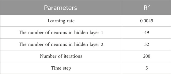
TABLE 2. Optimal parameter combination of BILSTM model.
4.3 Evaluation indicators
The model’s prediction accuracy is tested using three indicators: Root Mean Square Error (RMSE), Mean Absolute Error (MAE), and R_squared. The formulas for the three indicators are respectively:
4.4 Ablation experiments
This paper uses a mode of ablation experiment to assess the effectiveness of model improvement. Specifically, the example prediction is carried out with BILSTM, IWOA-BILSTM and the proposed model IWOA-SAA-BILSTM in this paper, respectively. In order to make the prediction results more scientific and reliable, the initial parameters of the BILSTM part of the three groups of models are kept consistent with part 7.1 during the experiment. In addition, the IWOA parameter settings of the IWOA-BILSTM model and the IWOA-SAA-BILSTM model were kept consistent. The model parameters were set, and the data was divided into training and test sets in an 8:2 ratio. After testing, the model stability before and after adding the IWOA optimization model is shown in Figure 8, and the IWOA model adaptation curve is shown in Figure 9:
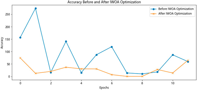
FIGURE 8. Model stability before and after IWOA optimization.
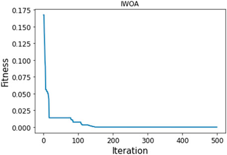
FIGURE 9. IWOA adaptation curve.
The model’s accuracy improved by IWOA has remained stable, with 90% of points now better than before, indicating a significant impact of IWOA on model prediction accuracy. Figure 9 and Figure 10 reveal that IWOA has a significantly faster convergence speed than WOA. IWOA has approached the optimal solution around the 140th iteration, while WOA needs to iterate 200 times to reach the optimal solution. The paper demonstrates the effectiveness of the proposed optimization method by highlighting the significant improvement in prediction efficiency and accuracy through the enhancement of WOA.
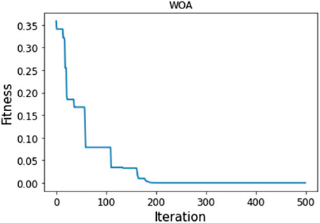
FIGURE 10. WOA adaptation curve.
Figure 11 displays the predicted and actual values of the IWOA-SAA-BILSTM model after three different model runs. By doing the ablation experiment with the other two groups of models, all the evaluation indexes of the models proposed in this paper are better than the other two groups of models. The ablation experiment demonstrates that the proposed model improvement can enhance the performance of the original model, thereby improving prediction efficiency and accuracy. Table 3 displays the evaluation indexes of the prediction results of the three model groups:
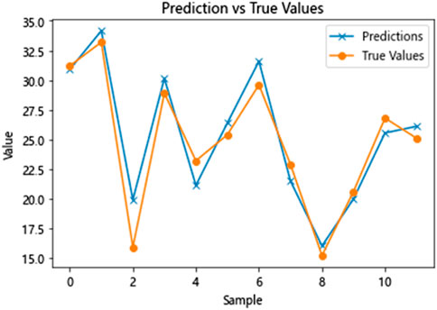
FIGURE 11. Plot of IWOA-SAA-BILSTM predicted values vs actual values.
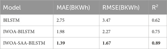
TABLE 3. Evaluation index values for BILSTM, IWOA-BILSTM, IWOA-SAA-BILSTM.
4.5 Comparative experiments
In addition to ablation experiments on the proposed model, this article also built several other commonly used models in existing research to demonstrate that the proposed model is not only superior to the pre-improved basic model, but also superior to common models in current research. This article selected four models with good performance in existing research, including WOA-SVM, WOA-LSTM, WOA-RBF, and WOA-ELM, as comparison models. The parameters of the IWOA-SAA-BILSTM model in this part of the experiment were kept consistent with the ablation experiment.
First, five groups of models were used to train the set, and the test set was used for fitting. The learning ability and fitting of the five groups of models for the data variation rule were compared. After the experiment, the loss function changes of the five groups of models are shown in the following figure.
Figure 12 provides a clear representation of the situation, the loss function of IWOA-SA-BILSTM is the smallest at the later stage of the iterative process, indicating that the model fitting effect of IWOA-SAA-BILSTM is superior to other models; and the loss function variation curve of IWOA-SAA-BILSTM decreases continuously with the increase of fitting times, until it reaches a stable state in the final stage of fitting, indicating that the IWOA-SAA-BILSTM model can correctly capture the data variation rules in the training data, has strong learning ability, and thus performs better prediction.
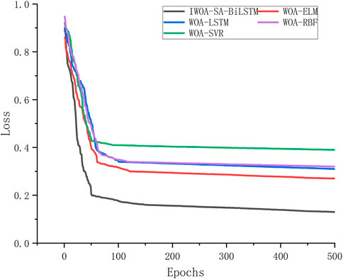
FIGURE 12. Loss function change curve diagram of five groups of models.
At the same time, using actual data for testing, we used evaluation indicators to measure the prediction accuracy and prediction accuracy of the five models. Table 4 displays the rating indicators of the four comparative models and the proposed model based on comparative experiments.
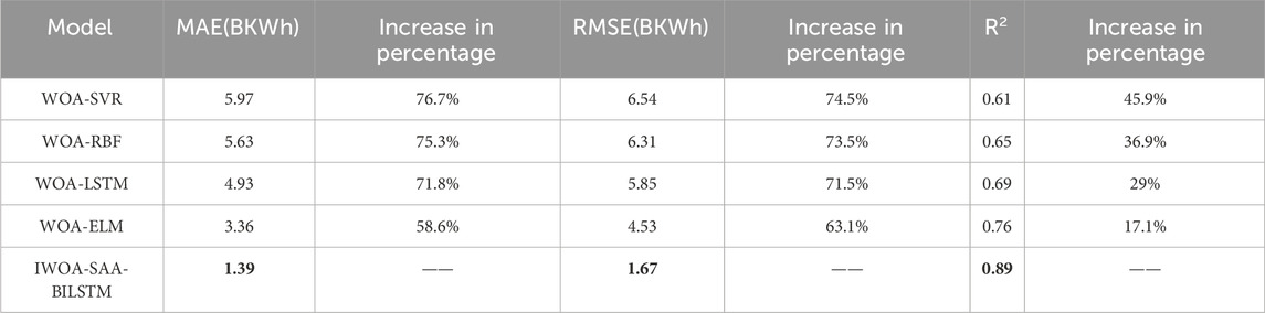
TABLE 4. Evaluation index value of each prediction model.
From the table, it can be seen that the prediction effects of IWOA-SAA-BILSTM are all better than the other four comparison models, with the optimal MAE value of 1.39 BKWh and the optimal RMSE value of 1.67 BKWh, this paper presents results that demonstrate the effectiveness of enhancing the standard whale optimization algorithm. And the R2 value shows that the effect of IWO-SAA-BILSTM prediction model is more stable. Therefore, the model proposed in this paper can be used as a favorable tool for renewable energy power load demand forecasting research.
4.6 Parameter sensitivity analysis
The model’s encoding dimension directly impacts the number of parameters and prediction performance. Therefore, analyzing the encoding dimension on the prediction performance of the model can help to find the optimal encoding dimension position, the model’s prediction performance has been enhanced.
Set the encoding dimensions to {32, 64, 128, 256, 512} and perform model operations separately. Use RMSE and MAE as evaluation metrics for model performance. The experimental results are shown in Figure 13.
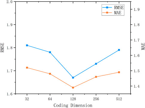
FIGURE 13. The influence of encoding dimensions on model performance.
As can be seen from the figure, when the model encoding dimension is 32 dimensions, the model is too simple and cannot learn enough effective data, resulting in poor model performance. Therefore, the model’s predictive performance can be enhanced by increasing its embedding dimension. When the encoding dimension is 128 dimensions, as can be seen from the figure, the prediction performance of the model is the best. This is because a higher model dimension can store more data information, allowing the model to better learn and simulate the regularities and changing characteristics of the data. However, an excessive encoding dimension is also not conducive to improving model performance. For example, when set to 256 dimensions and 512 dimensions, the prediction performance of the model decreases, which is due to the learning of excessive data noise and redundant information during data learning and feature simulation, affecting the prediction performance of the model.
Therefore, when the encoding dimension of the model is set to 128 dimensions, the IWOA-SAA-BILSTM model achieves the best prediction performance.
5 Conclusion
The objective is to enhance the precision of medium and short-term renewable energy power load demand forecasting, this article proposes an IWOA-SAA-BILSTM prediction model based on multi-dimensional feature analysis. Firstly, the factors that affect the renewable energy power load demand are screened, the study identifies the significant factors that significantly influence medium and short-term load demand. Then, the benchmark Whale Optimization Algorithm (WOA) is improved by adding Tent chaos mapping, and its internal convergence method is improved to be nonlinear, the improved Whale Optimization Algorithm (IWOA) has been obtained. Then, IWOA is used to optimize the weights of BILSTM, and Simulated Annealing Algorithm (SAA) is introduced to optimize the learning rate of BILSTM, the number of nodes in hidden layers 1 and 2 and the number of iterations are crucial factors to consider. The IWOA-SAA-BILSTM prediction model is obtained. At the end of the article, through case analysis, the prediction accuracy indicators of the model proposed in this article are: MAE is 1.39, RMSE is 1.67, and R_squared index is 0.89, which are all better than other comparison models. It shows that the prediction results of this model are reliable, and can provide corresponding theoretical basis for the research on renewable energy power load demand forecasting, as well as more theoretical guidance for power planning departments.
Data availability statement
The original contributions presented in the study are included in the article/Supplementary Material, further inquiries can be directed to the corresponding author.
Author contributions
MW: Writing–original draft. YX: Writing–original draft, Writing–review and editing. XZ: Writing–review and editing.
Funding
The author(s) declare financial support was received for the research, authorship, and/or publication of this article. This work was supported by the (Key Industry Innovation Chain Project of Shaanxi Provincial Department of Science and Technology), (Grant Number 22ZDLGY06); the (Shaanxi Provincial Philosophy and Social Science Research Specialized Key Issues), (2023HZ1659); the (Key Project of Philosophy and Social Sciences of Shaanxi Provincial Department of Education), (21JZ035); and the (Natural Science Foundation of Xi’an University of Architecture and Technology), (004/1603720032).
Conflict of interest
The authors declare that the research was conducted in the absence of any commercial or financial relationships that could be construed as a potential conflict of interest.
Publisher’s note
All claims expressed in this article are solely those of the authors and do not necessarily represent those of their affiliated organizations, or those of the publisher, the editors and the reviewers. Any product that may be evaluated in this article, or claim that may be made by its manufacturer, is not guaranteed or endorsed by the publisher.
Supplementary material
The Supplementary Material for this article can be found online at: https://www.frontiersin.org/articles/10.3389/fenrg.2023.1331076/full#supplementary-material
References
Dong, J. (2019). Demand response baseline load forecasting based on the combination of time series and kalman filter. Am. J. Electr. Power Energy Syst. 8 (3), 71. doi:10.11648/j.epes.20190803.11
Gao, G. (2023). Risk assessment due to load demand and electricity Price forecast uncertainty. Doctoral thesis (Glasgow, Scotland: University of Strathclyde).
Guo, X., Zhao, Q., Wang, S., Shan, D., and Gong, W. (2021). A short-term load forecasting model of LSTM neural network considering demand response. Q. Sun. Complex. 2021, 1–7. doi:10.1155/2021/5571539
He, M., Li, Y., and Zou, W. (2021). Application of ALO-ELM in load forecasting based on Big data. https://www.preprints.org/manuscript/202110.0302/v1.
He, Z., Lin, R., Wu, B., Zhao, X., and Zou, H. (2023). Pre-attention mechanism and convolutional neural network based multivariate load prediction for demand response. Energies Multidiscip. Digit. Publ. Inst. 16 (8), 3446. doi:10.3390/en16083446
Hu, S., Tang, H., Lu, K., et al. (2023). Deep belief network short-term load forecasting method considering generalized demand-side resources. Control theory Appl. 40 (3), 493–501. doi:10.7641/CTA.2021.10209
Hu, Z., Ma, J., Yang, L., Li, X., and Pang, M. (2019). Decomposition-based dynamic adaptive combination forecasting for monthly electricity demand. Sustainability 11 (5), 1272. doi:10.3390/su11051272
Luo, Y. (2018). Research on electricity demand forecasting based on structured data. Electron. Meas. Technol. 41 (12), 21–26. doi:10.19651/j.cnki.emt.1701420
Ma, T., Barajas-Solano, D. A., Huang, R., and Tartakovsky, A. M. (2022). Electric load and power forecasting using ensemble Gaussian process regression. J. Mach. Learn. Model. Comput. 3 (2), 87–110. doi:10.1615/jmachlearnmodelcomput.2022041871
Machado, E., Pinto, T., Guedes, V., and Morais, H. (2021). Electrical load demand forecasting using feed-forward neural networks. Energies 14 (22), 7644. doi:10.3390/en14227644
Moalem, S., Ahari, R. M., Shahgholian, G., Moazzami, M., and Kazemi, S. M. (2022). Long-term electricity demand forecasting in the steel complex micro-grid electricity supply chain—a coupled approach. Energies Multidiscip. Digit. Publ. Inst. 15 (21), 7972. doi:10.3390/en15217972
MuSAA, B., Yimen, N., Abba, S. I., Adun, H. H., and Dagbasi, M. (2021). Multi-state load demand forecasting using hybridized support vector regression integrated with optimal design of off-grid energy systems—a metaheuristic approach. Processes 9 (7), 1166. doi:10.3390/pr9071166
Qinghe, Z., Wen, X., Boyan, H., Jong, W., and Junlong, F. (2022). Optimised extreme gradient boosting model for short term electric load demand forecasting of regional grid system. Sci. Rep. 12 (1), 19282. doi:10.1038/s41598-022-22024-3
Rajbhandari, Y., Marahatta, A., Ghimire, B., Shrestha, A., Gachhadar, A., Thapa, A., et al. (2021). Impact study of temperature on the time series electricity demand of urban Nepal for short-term load forecasting. Appl. Syst. Innov. 4 (3), 43. doi:10.3390/asi4030043
Sekhar, C., and Dahiya, R. (2023). Robust framework based on hybrid deep learning approach for short term load forecasting of building electricity demand. Energy 268, 126660. doi:10.1016/j.energy.2023.126660
Shang, F., Yang, Z., Cheng, H., et al. (2015). Application of improved Verhulst model in saturated load forecasting. J. Power Syst. Automation 27 (1), 64–68. doi:10.3969/j.issn.1003-8930.2015.01.012
Shi, J., Lee, W.-J., Liu, Y., Yang, Y., and Wang, P. (2012). Forecasting power output of photovoltaic systems based on weather classification and support vector machines. IEEE TranSAActions Industry Appl. 48 (3), 1064–1069. doi:10.1109/tia.2012.2190816
Shi, J., Xie, L., and Wang, Z. (2019). Research on short-term load forecasting of industrial parks under construction based on the combination of discriminant analysis and support vector machine. Technol. innovation Appl. (10), 61–62. doi:10.3969/j.issn.2095-2945.2019.10.023
Su, C., Jin, C., Bian, S., et al. (2023). Power demand load forecasting method based on multi-feature fusion coding. Small Microcomput. Syst., 1–9.
Trull, O., García-Díaz, J. C., and Troncoso, A. (2021). One-day-ahead electricity demand forecasting in holidays using discrete-interval moving seasonalities. Energy 231, 120966. doi:10.1016/j.energy.2021.120966
Wen, J., Xian, Z., Chen, K., and Luo, W. (2022). A novel forward operator-based Bayesian recurrent neural network-based short-term net load demand forecasting considering demand-side renewable energy. Front. Energy Res. 10, 963657. doi:10.3389/fenrg.2022.963657
Yin, M., Ke, P., and Zhang, C. (2023). An improved whale optimization algorithm integrating multiple strategies. J. Wuhan Univ. Sci. Technol. 46 (2), 145–152. doi:10.3969/j.issn.1674-3644.2023.02.009
Zare-Noghabi, A., Shabanzadeh, M., and Saangrody, H. (2019). “Medium-term load forecasting using support vector regression, feature selection, and symbiotic organism search optimization,” in 2019 IEEE Power & Energy Society General Meeting (PESGM), Atlanta, GA, USA, August, 2019.
Zhang, S., Liao, X., and Cheng, Y. (2021b). Research on short-term power demand forecasting method of LSTM neural network based on characteristic analysis. Electr. Power Big Data 24 (5), 9–17. doi:10.19317/j.cnki.1008-083x.2021.05.002
Zhang, S., Wang, F., Zhu, Y., et al. (2022). Multi-regional power demand forecasting based on extreme gradient boosting. Comput. Mod. (3), 18–22+29. doi:10.3969/j.issn.1006-2475.2022.03.004
Zhang, T., and Gu, J. (2018). Markov short-term load forecasting method for high-proportion renewable energy power system. Grid Technol. 42 (4), 1071–1078. doi:10.13335/j.1000-3673.pst.2017.2479
Keywords: bi-directional long and short-term memory neural networks, whale optimization algorithm, multidimensional feature analysis, simulated annealing algorithm, load demand forecasting
Citation: Wang M, Xia Y and Zhang X (2024) Research on renewable energy power demand forecasting method based on IWOA-SA-BILSTM modeling. Front. Energy Res. 11:1331076. doi: 10.3389/fenrg.2023.1331076
Received: 31 October 2023; Accepted: 29 December 2023;
Published: 19 January 2024.
Edited by:
Rufeng Zhang, Northeast Electric Power University, ChinaReviewed by:
Linfei Yin, Guangxi University, ChinaGhulam Hafeez, University of Engineering and Technology, Pakistan
Copyright © 2024 Wang, Xia and Zhang. This is an open-access article distributed under the terms of the Creative Commons Attribution License (CC BY). The use, distribution or reproduction in other forums is permitted, provided the original author(s) and the copyright owner(s) are credited and that the original publication in this journal is cited, in accordance with accepted academic practice. No use, distribution or reproduction is permitted which does not comply with these terms.
*Correspondence: Minghu Wang, d2FuZ21pbmdodUB4YXVhdC5lZHUuY24=