Complex terrains and wind power: enhancing forecasting accuracy through CNNs and DeepSHAP analysis

Accurate prediction of wind power generation in regions characterised by complex terrain is a critical gap in renewable energy research. To address this challenge, the present study articulates a novel methodological framework using Convolutional Neural Networks (CNNs) to improve wind power forecasting in such geographically diverse areas. The core research question is to investigate the extent to which terrain complexity affects forecast accuracy. To this end, DeepSHAP—an advanced interpretability technique—is used to dissect the CNN model and identify the most significant features of the weather forecast grid that have the greatest impact on forecast accuracy. Our results show a clear correlation between certain topographical features and forecast accuracy, demonstrating that complex terrain features are an important part of the forecasting process. The study’s findings support the hypothesis that a detailed understanding of terrain features, facilitated by model interpretability, is essential for improving wind energy forecasts. Consequently, this research addresses an important gap by clarifying the influence of complex terrain on wind energy forecasting and provides a strategic pathway for more efficient use of wind resources, thereby supporting the wider adoption of wind energy as a sustainable energy source, even in regions with complex terrain.

1 Introduction

Wind energy is one of the most promising sources of renewable energy in the modern world. Its sustainability and low carbon footprint make it an attractive solution in the global effort to reduce greenhouse gas emissions and combat climate change (International Energy Agency IEA, 2022). As the penetration of wind energy increases, the ability to predict wind power generation becomes increasingly important for the operation of the electricity system. Accurate forecasting is essential not only to optimise energy production, but also to ensure grid stability and the successful integration of this variable energy source into power grids (Ahmed et al., 2020).

Forecasting wind power is a challenging task. The variability and unpredictability of wind, determined by many factors ranging from large-scale atmospheric dynamics to local geographical features, make it a complex phenomenon to predict. This challenge is even greater in regions with complex terrain. Mountains, valleys, coastlines and other topographic features add layers of complexity that can significantly affect wind patterns. For example, wind speeds can be amplified in mountain passes or become turbulent and erratic around steep cliffs and ridges. Predicting wind behaviour in such scenarios is critical, as these areas are often used to site wind farms due to their high wind potential. Traditional prediction models often fail to capture the nuanced interactions between wind and terrain (Bird et al., 2013; Hanifi et al., 2020).

As the demands on wind energy forecasting continue to grow, there is an urgent need for more advanced and accurate methods. While historical data and physical modelling have been the traditional basis for wind power prediction, the intricacies of wind behaviour in complex terrain require sophisticated computational techniques. In addition, to improve techniques, it is crucial to identify and understand the key factors that affect wind power forecasts. By identifying influential meteorological or geographical features, we can develop fine-tuned models that offer superior accuracy. This study uses a convolutional neural network (CNN) to predict wind power in areas with complex terrain. The aim is to address the unique challenges posed by these conditions and also to understand the factors that influence these predictions, in particular the relationship between terrain and wind dynamics.

2 Literature review

The study of wind power forecasting encompasses a wide range of methods, from classic time series analysis to cutting-edge machine learning strategies. Traditional techniques, in particular ARIMA, Exponential Smoothing and Vector Autoregression, have proven to be adept at adapting to the intricacies of complex terrain through their ability to capture the nuanced interplay between topography and wind flow. However, these methods have their limitations, particularly when it comes to accommodating a wide range of input variables and complex interdependencies between them (Chen et al., 2009).

Machine learning techniques have emerged in the field of wind energy forecasting and have been recognised for their ability to successfully deal with the complexity and non-linearities inherent in wind data (Wang et al., 2011; Giebel and Kariniotakis, 2017; Sideratos and Hatziargyriou, 2020; Tawn and Browell, 2022). From artificial neural networks to decision trees, support vector machines and advanced deep learning frameworks, these methods are redefining the benchmarks of forecast accuracy, especially in short-term forecast models. The advent of big data and cloud computing has further accelerated the adoption of advanced models, including convolutional and recurrent neural networks, leading to significant advances in regional wind power forecasting methodologies.

Several innovative techniques aimed at refining wind power forecasts have been presented in the literature. In (Ozkan and Karagoz, 2019), a data mining based strategy, known as the Regional Statistical Hybrid Wind Power Forecast Technique, is detailed for providing regional forecasts (Pinson et al., 2003). Presents a dynamic fuzzy neural network designed to improve forecast accuracy. In (Basu et al., 2020), a hybrid neural network model is developed that combines the capabilities of convolutional and multilayer perceptron networks for day-ahead forecasting. The study in (Dong et al., 2021) addresses the challenges of sparse data with a comprehensive approach, incorporating data correction and error analysis into a hybrid neural network to improve forecast accuracy. Furthermore, (Wood, 2022), presents a methodology that uses trend decomposition along with machine and deep learning for short-term wind capacity factor forecasting. Finally, (Yu et al., 2021), demonstrates the use of deep quantile regression for probabilistic forecasting, providing a robust method for dealing with forecast uncertainty. Deep learning has also been applied to wind speed forecasting, where the ability to predict and understand wind patterns is critical to the efficient operation of wind farms. In their seminal work, Wu et al. (2022a) presented an interpretable model for wind speed prediction using multivariate time series and temporal fusion transformers. This model is notable for its ability to process complex time-dependent data and provide insight into the temporal dynamics of wind speed, offering a significant advance over traditional methods. Similarly, Neshat et al. (2021) introduced a deep learning-based evolutionary model tailored for short-term wind speed forecasting at the Lillgrund offshore wind farm. Their approach combined the predictive power of deep neural networks with evolutionary algorithms to optimise the model’s performance, demonstrating a case study where deep learning models significantly improved the accuracy of wind speed predictions. These studies are part of a growing body of literature confirming the superiority of deep learning methods in predicting wind speed, especially when compared to classical statistical models. For example, a study by Zhang et al. (2019) used a deep learning framework to analyse wind turbine data and achieved remarkable success in predicting wind speed, thereby optimising turbine performance. Furthermore, a study by Lei et al. (2009) explored the application of convolutional neural networks to predict wind speeds, which not only improved prediction accuracy but also provided a better understanding of the spatial features relevant to wind speed variations.

Despite their effectiveness, simple ANN-based forecasting methods can struggle in complex terrain (Castellani et al., 2016; Clifton et al., 2022). Recent studies have highlighted the potential of deep learning to address these challenges. Toumelin et al. (2023) presented “DEVINE,” which uses CNNs to downscale weather forecasts with high-resolution topographic data, and demonstrated significant improvements in wind speed bias in complex terrain. Shin et al. (2023) emphasised the importance of spatio-temporal data for improving CNN forecasts, while Maldonado-Correa et al. (2021) and Eikeland et al. (2022) validated the effectiveness of hybrid models and the inclusion of historical weather data for probabilistic forecasting in difficult terrain. However, the use of ANNs has presented a paradoxical challenge. Although their performance exceeds that of traditional algorithms, the “black box” nature of their decision-making processes has attracted criticism (Montavon et al., 2017). The opacity of neural networks makes it difficult to discern the logic behind their accurate classifications and predictions, a significant problem in critical applications. To counter this, interpretive techniques such as DeepSHAP have emerged to provide a window into neural computation (Lundberg and Lee, 2017). DeepSHAP elucidates the influence of input features on model outputs, providing a level of transparency that enhances the interpretability of deep learning models (Doshi-Velez and Kim, 2017; Chen et al., 2018), thereby fostering confidence in their predictive capabilities.

3 Methodology

In this study, a methodology that evaluates terrain complexity metrics is developed for the region where wind power generation is expected. In conjunction with this, the DeepSHAP technique is applied to a CNN model to derive normalised importance values for the input features. These values are then compared to the terrain complexity matrices of the designated area. The primary goal is to integrate these methods to identify essential input features for wind power prediction and to discard redundant data from the input domain.

3.1 Convolutional neural networks

CNNs have reshaped the field of machine learning, particularly in tasks related to image and spatial data processing. Originally developed as a computational model for vision, CNNs are specifically designed to recognise and extract hierarchical patterns from structured, grid-like data (Alzubaidi et al., 2021). This makes them an ideal candidate for processing spatial data, such as images, where pixel relationships are essential, or, more relevant, weather grids, where spatial correlations between meteorological factors play a key role in forecasting. The cornerstone of CNNs lies in their ability to use convolutional layers to scan the input data with filters that detect local patterns. These patterns, initially simple in the early layers (such as edges or textures in images), become increasingly abstract and complex as the data progresses through deeper layers. This hierarchical pattern recognition is particularly useful for weather grids, where local interactions between variables such as temperature, pressure, and wind speed can lead to larger regional phenomena. In essence, CNNs can automatically and adaptively learn spatial hierarchies from the data, eliminating the need for manual feature engineering.

For the task of forecasting wind power generation, a simple CNN architecture is used that is suitable for handling the complexities of numerical weather predictions (Wang et al., 2022). The model consists of the following layers:

• Input layer: Accepts numerical weather predictions grids with dimensions representing spatial coordinates (latitude, longitude) and depth indicating various meteorological variables (e.g., wind speed, wind direction).

• Convolutional layers: Multiple layers are used, each with a set of filters to extract relevant features from the input data. The ReLU (Rectified Linear Unit) is used as the activation function to introduce nonlinearity.

• Pooling layers: Interspersed with the convolutional layers, these layers downsample the spatial dimensions, preserving essential information while reducing the computational burden. In this work, max-pooling was used, which retains the maximum value from each local region.

• Fully connected layers: Following the convolutional and pooling layers, one or more fully connected layers interpret the extracted features and drive the prediction mechanism.

• Output layer: Provides the wind power generation prediction for the region of interest.

Based on these characteristics, CNNs fundamentally revolve around a sequence of mathematical operations for processing spatial data, as presented in Eqs (1–9).

1. Convolution operation: Given an input matrix I (representing a small section of our spatial data) and a filter matrix F, the convolution operation is defined as follows:

$\left(I*F\right)\left(r,z\right)={\displaystyle \sum _{i=-\infty }^{\infty }}{\displaystyle \sum _{j=-\infty }^{\infty }}I\left(i,j\right)\cdot F\left(r-i,z-j\right)(1)$

For most applications, I and F are 2D matrices, and the convolution operates throughout the spatial extent of I.

2. Activation function: Post-convolution, an activation function is applied element-wise to introduce nonlinearity. One of the most popular is the Rectified Linear Unit (ReLU):

$ReLU\left(x\right)=\max \left(0,x\right)(2)$

3. Pooling operation: Pooling layers reduce the spatial dimensions of the feature maps. For example, the max-pooling operation is defined as:

$\begin{array}{ll}\hfill MaxPool\left(I\right)\left(r,z\right)& =\max \left(I\left\{i,j\right\}\forall i,j\in \left[r,r+W\right],\right.\hfill \\ \hfill & \left.j\in \left[z,z+H\right]\right)\hfill \end{array}(3)$

where W and H are the width and height of the pooling window, respectively.

4. Fully Connected Layers: In these layers, neurons are densely connected. Given an input vector X, weights A, and biases b, the output Y for a fully connected layer is:

$Y=A\cdot X+b(4)$

Integrating these mathematical formulations, a CNN processes spatial data through convolution and pooling operations, introduces non-linearity through activation functions, and uses fully connected layers for final predictions, all while minimising a specified regression loss function. Batch normalisation and dropout techniques have also been incorporated into the architecture to ensure model stability and prevent overfitting. The general architecture of the proposed CNN model is shown in Figure 1. The convolution and pooling layers contained 16 filters with a kernel size of 3 in all dimensions, and the fully connected layers contained 100 nodes each. The model was trained using the Adam optimiser (learning rate = 0.01) with a mean squared error loss function, which is particularly suitable for regression tasks.

FIGURE 1

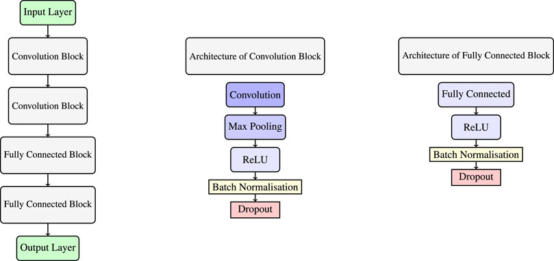
FIGURE 1. Architecture of the proposed CNN model.

3.2 DeepSHAP

3.2.1 Explainable AI in general

As deep learning models become increasingly sophisticated, their predictions can often be hard to interpret, earning them the moniker “black-box” models. In critical applications, such as medical imaging, power system operation or finance, understanding the reasoning behind these predictions is crucial. This need for interpretability has led to Explainable AI (XAI), an interdisciplinary field that aims to make AI decision making transparent, interpretable and trustworthy (Arrieta et al., 2020). One prominent method in XAI is the concept of Shapley values, which originated from cooperative game theory. Imagine a group of workers working on a project. The Shapley value determines how much each worker contributed to the project success, considering all possible collaborations. In the context of machine learning, each “worker” is a feature and the “project’s success” is the prediction. The Shapley value for a feature is then computed on the basis of its marginal contribution across all possible combinations of features. Mathematically, the Shapley value for a feature i is defined as

${\varphi }_i\left(f\right)={\displaystyle \sum _{S\subseteq N\backslash i}}\frac{|S|!\left(|N|-|S|-1\right)!}{|N|!}\left[f\left(S\cup i\right)-f\left(S\right)\right](5)$

where f is the prediction function, N is the set of all features, and S is a subset of N without feature i. However, computing Shapley values can be computationally demanding, especially for DNN with numerous input features (Castro et al., 2009). Here DeepSHAP offers an efficient approximation by using a process analogous to backpropagation (Goodfellow et al., 2016).

3.2.2 DeepSHAP propagation in neural networks

DeepSHAP aims to approximate Shapley values for DNN, particularly feedforward neural networks. It does so by redistributing the Shapley values from the output through the network to the inputs (Lundberg and Lee, 2017). This backward pass redistributes the importance or contributions of the output rather than gradients. When attributing the contribution of neuron activations to their respective inputs, the activation of one neuron and the weight of the connection to the next must be accounted for. Mathematically:

${\varphi }_{i\to j}={\displaystyle \sum _k}{\varphi }_{j\to k}\times \frac{a_i\times w_{i,k}}{{\sum }_l{a}_l\times w_{l,k}}(6)$

where ϕ_i→j is the Shapley value of neuron i contributing to neuron j, ϕ_j→k is the Shapley value of neuron j contributing to neuron k, a_i is the activation of neuron i, w_i,k is the synaptic weight connecting neurons i and j, k an index referring to neurons that neuron j contributes to and l an index for summation, referring to all neurons that are inputs to neuron k.

Convolutional layers, prevalent in deep learning models for image processing, introduce an additional layer of complexity due to shared weights across spatial dimensions. Therefore, DeepSHAP must account for spatial relationships when redistributing contributions. For a specific convolutional filter applied across an input feature map, the contribution of a particular input pixel to an output pixel depends on the filter’s weights and the relative position of the pixels. This relationship is described by:

${\varphi }_{r,z}^{\mathit{input}}={\displaystyle \sum _{i,j}}{\varphi }_{i,j}^{\mathit{output}}\times \frac{I_{r,z}\times F_{i-r,j-z}}{{\sum }_{p,q}{I}_{p,q}\times F_{i-p,j-q}}(7)$

where ${\varphi }_{r,z}^{\mathit{input}}$ is the Shapley value for the pixel at position (r, z) in the input feature map, ${\varphi }_{i,j}^{\mathit{output}}$ is the Shapley value for the pixel at position (i, j) in the output feature map, I_r,z is the pixel value at position (r, z) in the input feature map, F_i−r,j−z is the weight of the convolutional filter at the relative position to the input pixel, i and j are indices referring to positions in the output feature map, p and q are indices for summation, referring to all positions in the input feature map that contribute to a specific output position.

DeepSHAP’s treatment of convolutional layers provides a detailed perspective into which patterns or regions in input feature maps are pivotal for the model’s decision, considering not just the importance of a feature but its spatial context in the decision-making process.

3.3 Terrain complexity metrics

The complexity of a terrain can significantly influence the environmental and atmospheric dynamics, especially wind patterns. Several metrics have been developed to quantify different aspects of this complexity. Understanding these metrics is crucial when integrating them with advanced machine learning techniques, such as DeepSHAP, to decipher the intricate interplay between terrain and wind dynamics. The importance of these terrain metrics in various environmental processes has been highlighted by several studies (Stock and Dietrich, 2006; Wu et al., 2022b).

• Topographic Ruggedness Index (TRI): This index measures roughness based on elevation variances between a cell and its neighboring cells (Riley et al., 1999). Mathematically, it’s expressed as:

$TRI=\sqrt{{\displaystyle \sum _{i=1}^n}{\left(a_i-a_{\mathit{mean}}\right)}^2}(8)$

where a_i denotes the elevation of cell i, and a_mean represents the mean elevation of all adjacent cells. The value of n corresponds to the number of cells considered.

• Standard Deviation of Elevation (SDE): A rudimentary metric, it calculates the standard deviation of elevation values within a specified area (Jenny and Hurni, 2011), symbolised as:

$SDE=\sqrt{\frac{1}{N}{\displaystyle \sum _{i=1}^N}{\left(a_i-\mu \right)}^2}(9)$

where a_i is each elevation value, N is the total number of values and μ is the mean elevation.

In the context of wind power prediction using CNN and DeepSHAP, these terrain complexity metrics play a key role. DeepSHAP determines the importance of each feature by calculating the Shapley values from the output to the input layer. For spatial datasets, such as numerical weather predictions, this reveals which regions or patterns are critical to the model’s decision. Comparing DeepSHAP’s feature importance values with terrain complexity indices can be revealing. For example, areas identified as high importance by DeepSHAP, when overlaid with regions with high TRI or SDE values, could indicate the importance of rugged terrain in influencing wind power predictions. In essence, if a complex terrain metric closely matches DeepSHAP importance values in a region, it suggests that terrain complexity is a dominant factor in model decisions in that area. Such an investigation provides an empirical way to understand how terrain undulations and complexity affect wind predictability and variability. As a result, prediction models can be refined to ensure that they are better suited to the unique challenges posed by different terrains.

4 Case studies

Exploring the complexities of predicting wind power generation requires an in-depth understanding of the complex interaction between atmospheric conditions and different terrain features. In this context, the selection of Greece, Bulgaria and Romania as our case studies provides a unique opportunity. These countries, each with their own topographical characteristics, provide a diverse landscape for our investigation. Greece’s landscape is a mixture of rugged mainland terrain, numerous islands and extensive coastlines. Bulgaria, on the other hand, offers a mix of mountainous regions and flat plains, while Romania’s topography is characterised by the Carpathian Mountains, rolling hills and vast plains. This diversity in the geography of these countries allows for a more comprehensive analysis and helps us to understand regional differences in wind power generation.

Recognising that topographic complexity is shaped by a range of factors beyond simply elevation, a comprehensive set of metrics is employed. These include elevation maps, which capture the variation in elevation from coastlines to mountain peaks in all three countries. In addition, metrics such as the TRI and SDE are used to quantify the ruggedness and heterogeneity of each terrain. Shifting focus, the second analysis evaluates the capabilities of a CNN trained on numerical weather predictions and regional wind power generation measurements for Greece, Bulgaria and Romania, as shown in Table 1. The primary objective of this training is to accurately predict regional wind power generation. The input features for each case study consist of wind speed and direction forecasts at a height of 10 m, obtained from the Global Forecast System (GFS). These forecasts are structured in a 3D grid format, where the first two dimensions represent the geographical coordinates (latitude and longitude) covering the respective region, and the third dimension contains the wind speed and direction forecasts. This 3D grid is essentially an image-like array that the CNN interprets in a similar way to a visual image. During the training phase, this 3D grid is fed into the CNN, allowing the model to learn the spatial and temporal patterns of wind behaviour in the different terrains of the three countries. The model is trained to recognise how these patterns correlate with actual wind power generation, a crucial step in making accurate predictions. The output data for the model comes from the ENTSO-e platform, which provides actual measurements of the wind power generated in each region. This output is normalised by the installed capacity in each area to standardise the data and ensure that the model’s predictions are proportionate and comparable across different regions with different capacities.

TABLE 1

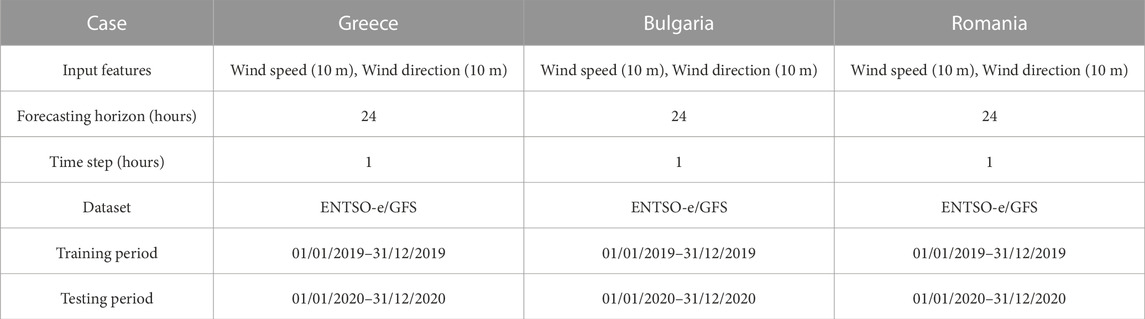
TABLE 1. Case study information.

However, achieving high prediction accuracy is only one aspect of the objective; it is equally important to understand which input features the model considers critical for its predictions. To this end, we use DeepSHAP to generate Feature Importance Factors (FIV). This technique provides insight into which aspects of numerical weather prediction have the most influence on the model’s prediction process. The third analysis attempts to combine the results of the previous two analyses. The feature importance matrices produced by DeepSHAP are compared with the terrain complexity matrices for each country. This comparison will highlight the extent to which terrain complexity affects the importance of different input variables in the prediction model. Such an integrative approach allows us to draw more holistic conclusions about the interaction between terrain complexity and wind energy production in different geographical landscapes.

5 Results

5.1 Terrain complexity

The analysis of terrain complexity in Greece, Bulgaria and Romania is visually summarised in Figure 2 (Greece), 3 (Bulgaria) and 4 (Romania). The left sub-figures display the elevations map of each country. The middle sub-figures display the TRI, highlighting areas of significant topographic variability. Finally, the right sub-figures display the SDE of each country, which provides a quantitative perspective on elevation variability within each region shown. These visual representations serve as a foundation for understanding the complicated relationship between terrain complexity and wind energy prediction in these different geographical areas.

FIGURE 2

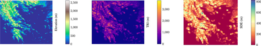
FIGURE 2. Elevation and terrain complexity metrics over the extended area of Greece.

In Greece (Figure 2), the elevation map shows a high contrast between high mountain peaks and sea level, indicative of the mountainous regions of the country and the extensive coastline. The TRI highlights the regions of Greece that are particularly variable in topography, which is likely to have a significant impact on wind flow patterns. The SDE further quantifies these variations, painting a picture of the ruggedness of the terrain. Moving to Bulgaria (Figure 3), the elevation map shows a mixture of flat plains and mountain areas, the TRI highlighting the variability of the Balkan Mountains. The SDE for Bulgaria reflects a more uniform landscape in the plains, with pockets of complexity in the mountainous areas, which could indicate localised areas of more unpredictable wind behaviour. Finally, Romania’s landscape (Figure 4) is captured by an elevation map that outlines the extensive Carpathian mountain range as well as the lower elevation regions. The TRI highlights the complexity of the Carpathians, which may correlate with areas of complex wind patterns. The SDE map confirms this complexity, with variability in elevation that can affect both micro- and macro-scale wind flows.

FIGURE 3

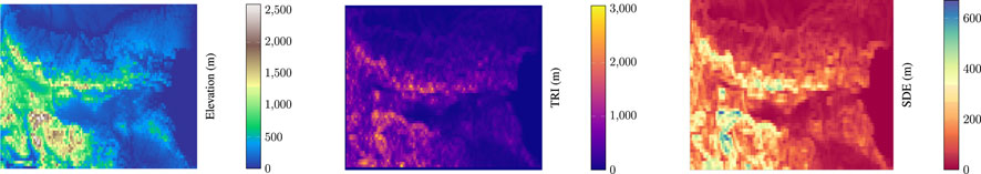
FIGURE 3. Elevation and terrain complexity metrics over the extended area of Bulgaria.

FIGURE 4

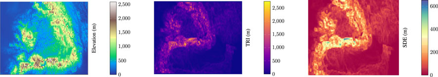
FIGURE 4. Elevation and terrain complexity metrics over the extended area of Romania.

5.2 Feature importance analysis

In this analysis, we examine the influence of terrain complexity on wind power prediction by analysing the normalised FIV for Greece, Bulgaria and Romania. Figures 5, 6 show a comparison of these values for wind speed and wind direction predictions in relation to the topographic metrics of each country. In the case of Greece (Figure 5, left), the FIV of the elevation map shows a higher importance in coastal areas and a lower importance in the mountainous regions. This suggests that while the highlands contribute to wind variability, it is the coastal areas where consistent wind patterns dominate the model’s focus, possibly due to the unobstructed flow of sea breezes that are crucial for wind power generation. The TRI visualisation further supports this by showing less importance in regions with high topographic variability, suggesting that CNN may find it difficult to predict wind patterns where the terrain is most rugged. For wind direction (Figure 6, left), the FIV is particularly significant along the sea coast, highlighting the importance of offshore influences on the wind pattern for both the mainland and the islands. In the case of Bulgaria (Figure 5, middle), the FIV for wind speed suggests that the model assigns different degrees of importance across the country, reflecting Bulgaria’s combination of flat terrain and mountainous areas. Areas of significant FIV align with regions of lower topographic complexity, suggesting that in Bulgaria, unlike Greece, the simpler terrain of the interior may provide more reliable wind conditions for power generation. The values of the importance of the wind direction (Figure 6, middle) show a scattered pattern, suggesting that the impact of wind direction on power forecasting is influenced by the combination of the Balkan Mountains and the surrounding plains. The Romanian analysis (Figure 5, right) shows a clear distribution of FIV across the Carpathians and the vast plains. The model places less emphasis on wind speed predictions in the highly complex Carpathian region, possibly due to the unpredictability of wind behaviour in such terrain. On the contrary, the plains, with their more predictable wind patterns, receive higher FIV scores. For wind direction (Figure 6, right), the FIV is noticeably concentrated in areas that serve as natural wind corridors, suggesting that certain flat and valley regions are key to the prediction process of the prediction model. It is clear that while complex terrain can introduce forecast variability, consistent and predictable wind patterns, particularly in maritime regions, are critical in shaping the focus of the forecast model. This underscores the importance of considering both land- and sea-based influences in the development of accurate wind power forecasts.

FIGURE 5

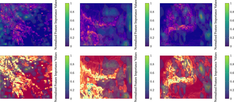
FIGURE 5. Display of Normalised feature importance values of wind speed predictions over the ruggedness metrics’ maps of all case studies (Left: Greece, Middle: Bulgaria, Right: Romania).

FIGURE 6

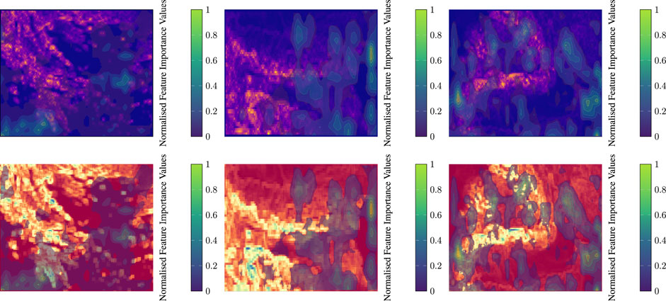
FIGURE 6. Display of Normalised feature importance values of wind direction predictions over the ruggedness metrics’ maps of all case studies (Left: Greece, Middle: Bulgaria, Right: Romania).

5.3 Forecasting performance

Using the knowledge from the feature importance and terrain complexity analysis, the proposed work is focussing on the refinement of the input data by emphasising areas of significance while filtering out potential noise can significantly enhance a model’s performance. In our efforts to optimise the input for a CNN model, we systematically investigated three approaches. Each method contains its own unique philosophy, based on computational insights derived from the model or observations of the landscape. The basic goal remained the same: to mask out inputs that help the model deliver accurate wind power forecasts. The following sections clarify these three correspondences and the rationale behind their design.

5.3.1 Approach 1: feature selection based on FIV using DeepSHAP

To improve the predictive accuracy of our CNN model for wind power forecasting, our first approach exploits the strategic use of FIV as determined by DeepSHAP. This method is based on the premise that not all regions within the input data contribute equally to the model’s predictions. In particular, regions with low FIVs, as identified by DeepSHAP, are considered to have a minimal or even detrimental effect on prediction accuracy. These regions could represent noise or irrelevant information that could potentially bias the model performance (Lundberg and Lee, 2017; Molnar, 2020). To implement this approach, we applied a selective filtering process to the training data on the key weather variables: wind speed and wind direction. For each of these variables, we examined the normalised FIV values across the input grid. Areas where the FIV was below a threshold of 0.2 were considered to be of low importance. To mitigate their influence, we set the values in these areas to a placeholder or dummy value of −1. This value acts as a signal to the model, effectively “masking” these regions during the training process. The motivation for this decision is twofold. Firstly, by reducing the influence of less important regions, we reduce the likelihood of the model being misled by noise or irrelevant data points. Secondly, and more importantly, this approach sharpens the model’s focus on higher FIV regions, which are theoretically more important in determining accurate wind power forecasts. This method is consistent with the strategies adopted in recent studies where researchers have successfully used feature selection techniques based on importance values to streamline model training and improve overall accuracy.

5.3.2 Approach 2: data filtering based on terrain complexity

The second approach focuses on the dynamic relationship between terrain complexity and wind behaviour, an aspect less emphasised in traditional models. Instead of relying exclusively on FIV, this method integrates SDE as a key metric to assess terrain complexity. This approach is based on the hypothesis that regions with less rugged terrain, as indicated by a lower SDE, are likely to have more predictable and consistent wind profiles. In contrast, areas with a higher SDE, indicating greater ruggedness, may contribute to the unpredictability of wind patterns. To incorporate this terrain-based information into our CNN model, we manipulated the input training data for both wind speed and wind direction. Specifically, regions with an SDE value greater than 400 m were assigned a dummy value of −1. This threshold of 400 m, determined based on the average SDE in each region under study as shown in Figure 2, serves as an arbitrary yet strategic boundary to differentiate between areas of low and high terrain complexity. By applying this filter, we aim to sharpen the focus of the model, allowing it to focus on regions where terrain complexity is less likely to distort wind patterns. By selectively masking regions with high SDE values, we potentially enhance the ability of the model to recognise and adapt to the varying effects of terrain complexity on wind dynamics.

5.3.3 Approach 3: integrating FIV and terrain complexity for improved data filtering

Approach 3 represents a synergistic integration of the first two methods, merging the model-driven insights derived from FIV with the empirical understanding of terrain complexity as indicated by SDE. This approach is based on the premise that a more robust and accurate forecast model can be achieved through a more sophisticated data filtering process that takes into account both the learned patterns of the model and the physical characteristics of the terrain. In practice, this integrated approach involves a two-step filtering mechanism applied to the input training data. First, for each weather variable—wind speed and wind direction—the regions where the normalised FIV falls below the threshold of 0.2 are identified. The values in these regions are then set to −1, effectively “masking” them in the training data set. This step is based on the principle that regions with low FIV contribute less to the model’s predictive accuracy and may even act as noise, affecting the model’s performance. Following the initial FIV-based filtering, the approach further incorporates considerations of terrain complexity. Areas where the SDE exceeds a predefined threshold of 400 m are also assigned a value of −1. This threshold was chosen to distinguish regions with significant terrain variation from those with more uniform topographic features. The choice of 400 m as a threshold is strategic, as it aims to filter out regions where complex terrain could introduce unpredictability in wind patterns, potentially complicating the forecasting task. By combining these two filtering criteria, Approach 3 creates a training dataset that is both selective and strategic. It emphasises regions that are not only considered important by the model (as per high FIV), but also those with less complex terrain (as per low SDE), and thus potentially more predictable in terms of wind behaviour. This refined dataset is expected to guide the CNN model to focus on the most relevant and reliable features for wind power prediction, thereby improving its overall prediction accuracy.

5.3.4 Evaluation results

To objectively assess the efficacy of the three data preprocessing approaches, a set of reliable evaluation metrics was used. Normalised mean absolute error (NMAE) and normalised mean squared error (NMSE) were used to gain an understanding of the average magnitude of errors and the model prediction accuracy (Willmott and Matsuura, 2005; Chai and Draxler, 2014). The NMAE indicates the average absolute discrepancy, while the NMSE magnifies the effect of larger errors, thus providing an indication of the model’s forecast reliability (Hyndman and Koehler, 2006). Additionally, the standard deviation was calculated to measure the variability or spread of prediction errors and to assess the consistency of the model’s forecasting ability. The bias was also calculated to identify any systematic overprediction or underprediction tendencies in the model. To compare the performance of the three approaches, metrics were calculated and compared to a baseline scenario, where the input training data was not masked. Through this comparative analysis, our objective is to determine the added value, if any, of the data preprocessing steps.

6 Discussion

The comparative analysis of data processing approaches in Greece, Bulgaria and Romania, as shown in Tables 2–4, provides a detailed evaluation of their impact on CNN-based wind power forecasting.

TABLE 2

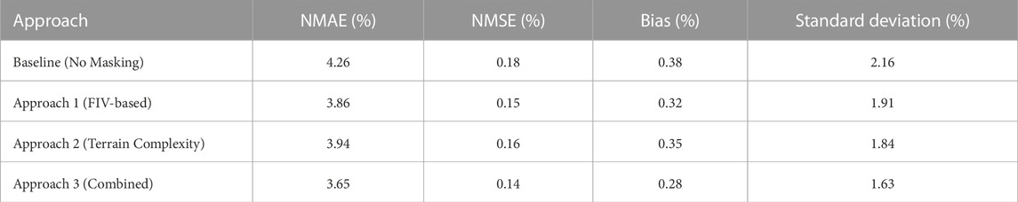
TABLE 2. Case study: Greece—evaluation results for the three approaches.

TABLE 3

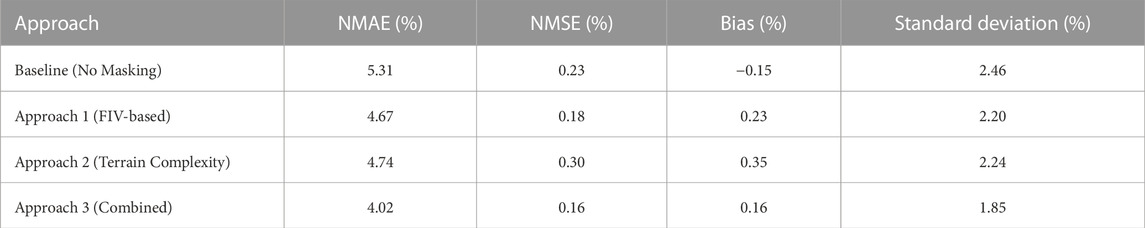
TABLE 3. Case study: Bulgaria—evaluation results for the three approaches.

TABLE 4

TABLE 4. Case study: Romania—evaluation results for the three approaches.

In Greece (Table 2), the baseline approach sets the standard for comparison, with an NMAE of 4.26% and an NMSE of 0.18%. The bias and standard deviation provide information on the average prediction error of the model and its variability. After implementing Approach 1, which incorporates FIV-based data filtering, a reduction in all metrics is observed, indicating improved accuracy and model stability. Approach 2, which focusses on terrain complexity, yields improvements but falls short of the gains made by Approach 1, suggesting the dominance of FIV-driven regions in influencing wind pattern predictions. However, Approach 3, which combines both FIV and terrain complexity considerations, outperforms the individual approaches, achieving the lowest NMAE, NMSE, bias and standard deviation, thereby demonstrating superior forecast performance and reliability. For Bulgaria (Table 3), the baseline metrics are higher compared to Greece, indicating a greater initial error in the predictions. The adaptation of Approach 1 again proves to be beneficial, as evidenced by the lower NMAE and NMSE. Interestingly, Approach 2 leads to an increase in NMSE despite a reduction in other metrics, suggesting a complex interaction between the features and the terrain. However, Approach 3 emerges as the most effective, significantly reducing all metrics, highlighting the value of a hybrid approach that uses both model-driven and empirical data insights. The results for Romania (Table 4) show the highest baseline NMAE and NMSE of the three countries, highlighting initial challenges in the forecasting model due to possibly more complex wind patterns or varied terrain. Approach 1 and Approach 2 show improvements, but Approach 2 shows a negative NMSE value that may require further investigation to understand anomalous model behaviour. Approach 3 demonstrates its robustness by significantly improving the accuracy and consistency of the forecast, as indicated by significant reductions in all metrics.

The results of the analysis from Greece, Bulgaria and Romania clearly indicate that a hybrid approach combining both FIV and terrain complexity metrics consistently improves CNN-based wind power prediction. This combined strategy, as shown by the data in Tables 2–4, consistently outperforms the individual use of either FIV or terrain complexity metrics alone. The singular use of FIV-based data filtering (Approach 1) while beneficial in reducing error metrics such as NMAE and NMSE, may not fully capture the diverse influence of complex terrain on wind patterns. Similarly, Approach 2 by focusing exclusively on terrain complexity provides a limited view and occasionally leads to inconsistent results, such as the unexpected increase in NMSE for Bulgaria. It is the fusion of both approaches that provides a comprehensive understanding, integrating the data-driven insights of FIV with the empirical knowledge of terrain effects. This dual strategy exploits the strengths of both approaches: FIV’s ability to identify predictive regions within the data, and the complexity of the terrain, which reflects the geographical influence on wind behaviour. The superior performance of Approach 3 in all three countries underlines the synergy achieved by combining these methods. It fine-tunes the forecast model to account for the unique geographical characteristics of each region, resulting in more accurate, reliable and interpretable wind power forecasts. The consistent improvement across all metrics with this combined approach confirms its effectiveness and demonstrates the value of integrating different data processing methods to improve forecasting capability in complex, real-world applications.

7 Conclusion

This research conducted a comprehensive study of the interaction between terrain complexity and feature importance values derived from deep learning models, with a particular focus on their collective impact on wind power predictions. Convolutional Neural Networks using numerical weather prediction were used to extract the intricate correlations influencing wind power generation in Greece, Bulgaria and Romania. The research used metrics such as Standard Deviation of Elevation and Terrain Ruggedness Index, which showed a discernible effect on wind behaviour across the diverse landscapes of these countries. The feature importance analysis, facilitated by the DeepSHAP methodology, identified critical areas within each country that had a significant impact on the forecasting process. A consistent pattern emerged from the analysis; regions with pronounced rugged terrain, particularly inland, generally showed reduced importance. In contrast, maritime regions emerged as a significant contributor to wind dynamics, underlying the importance of coastal and marine areas in the forecast models. The study tested three data filtering approaches to improve forecast accuracy: one based on FIV, another based on terrain complexity, and a third that combined both sets of approaches. Across all case studies, the combined method proved superior, consistently outperforming the others by providing the most accurate forecasts, minimising errors and reducing variability of results. This method effectively combines the data-driven focus of FIV with the empirical knowledge of the field, providing a robust framework for forecasting. In general, this research highlights the value of integrating terrain characteristics with deep learning-derived algorithmic predictions. By adopting such an integrated approach, the potential for optimising wind energy forecasting is greatly enhanced, offering a way to improve the sustainability of energy resources in regions characterised by complex terrain.

Data availability statement

Publicly available datasets were analyzed in this study. This data can be found here: https://www.ncei.noaa.gov/products/weather-climate-models/global-forecast, https://transparency.entsoe.eu/generation/r2/actualGEnerationPerProductionTYpe/show?name=&defaultValue=true&viewType=TABLE&areaType=BZN&atch=false&datepicker-day-offset-select-dv-date-from_input=D&dateTIme.dateTime=24.10.2023+00:00|CET|DAYTIMERANGE&dateTIme.endDAteTime=24.10.2023+00:00|CET|DAYTIMERANGE&area.values=CTY|10YGR-HTSO-----Y!BZN|10YGR-HTSO-----Y&productionTYpe.values=B01&productionTYpe.values=B02&productionTYpe.values=B03&productionTYpe.values=B04&productionTYpe.values=B05&productionTYpe.values=B06&productionTYpe.values=B07&productionTYpe.values=B08&productionTYpe.values=B09&productionTYpe.values=B10&productionTYpe.values=B11&productionTYpe.values=B12&productionTYpe.values=B13&productionTYpe.values=B14&productionTYpe.values=B20&productionTYpe.values=B15&productionTYpe.values=B16&productionTYpe.values=B17&productionTYpe.values=B18&productionTYpe.values=B19&dateTIme.timezone=CET_CEST&dateTime.timezone_input=CET+(UTC+1)+/+CEST+(UTC+2), https://developers.google.com/maps/documentation/elevation/overview.

Author contributions

TK: Writing–original draft. NH: Writing–review and editing.

Funding

The author(s) declare that no financial support was received for the research, authorship, and/or publication of this article.

Conflict of interest

The authors declare that the research was conducted in the absence of any commercial or financial relationships that could be construed as a potential conflict of interest.

Publisher’s note

All claims expressed in this article are solely those of the authors and do not necessarily represent those of their affiliated organizations, or those of the publisher, the editors and the reviewers. Any product that may be evaluated in this article, or claim that may be made by its manufacturer, is not guaranteed or endorsed by the publisher.

References

Ahmed, S. D., Al-Ismail, F. S. M., Shafiullah, M., Al-Sulaiman, F. A., and El-Amin, I. M. (2020). Grid integration challenges of wind energy: a review. IEEE Access 8, 10857–10878. doi:10.1109/access.2020.2964896

CrossRef Full Text | Google Scholar

Alzubaidi, L., Zhang, J., Humaidi, A. J., Al-Dujaili, A. Q., Duan, Y., Al-Shamma, O., et al. (2021). Review of deep learning: concepts, cnn architectures, challenges, applications, future directions. J. Big Data 8, 53. doi:10.1186/s40537-021-00444-8

PubMed Abstract | CrossRef Full Text | Google Scholar

Arrieta, A. B., Díaz-Rodríguez, N., Del Ser, J., Bennetot, A., Tabik, S., Barbado, A., et al. (2020). Explainable artificial intelligence (xai): concepts, taxonomies, opportunities and challenges toward responsible ai. Inf. Fusion 58, 82–115. doi:10.1016/j.inffus.2019.12.012

CrossRef Full Text | Google Scholar

Basu, S., Watson, S., Lacoa Arends, E., and Cheneka, B. (2020). Day-ahead wind power predictions at regional scales: Post-processing operational weather forecasts with a hybrid neural network.

Google Scholar

Bird, L., Milligan, M., and Lew, D. (2013). Integrating variable renewable energy: challenges and solutions.

Google Scholar

Castellani, F., Astolfi, D., Mana, M., Burlando, M., Meißner, C., and Piccioni, E. (2016). “Wind power forecasting techniques in complex terrain: ann vs. ann-cfd hybrid approach,” in Journal of Physics: Conference Series, 753, 082002. doi:10.1088/1742-6596/753/8/082002

CrossRef Full Text | Google Scholar

Castro, J., Gomez, D., and Tejada, J. (2009). Polynomial calculation of the shapley value based on sampling. Comput. Intell. Games 36, 1726–1730. doi:10.1016/j.cor.2008.04.004

CrossRef Full Text | Google Scholar

Chai, T., and Draxler, R. R. (2014). Root mean square error (rmse) or mean absolute error (mae)? arguments against avoiding rmse in the literature. Geosci. Model Dev. 7, 1247–1250. doi:10.5194/gmd-7-1247-2014

CrossRef Full Text | Google Scholar

Chen, J., Song, L., Wainwright, M. J., and Jordan, M. I. (2018). Learning to explain: an information-theoretic perspective on model interpretation, 07814. CoRR abs/1802.

Google Scholar

Chen, P., Pedersen, T., Bak-Jensen, B., and Chen, Z. (2009). Arima-based time series model of stochastic wind power generation. IEEE Trans. power Syst. 25, 667–676. doi:10.1109/tpwrs.2009.2033277

CrossRef Full Text | Google Scholar

Clifton, A., Barber, S., Stökl, A., Frank, H., and Karlsson, T. (2022). Research challenges and needs for the deployment of wind energy in hilly and mountainous regions. Wind Energy Sci. 7, 2231–2254. doi:10.5194/wes-7-2231-2022

CrossRef Full Text | Google Scholar

Dong, W., Sun, H., Tan, J., Li, Z., Zhang, J., and Zhao, Y. Y. (2021). Short-term regional wind power forecasting for small datasets with input data correction, hybrid neural network, and error analysis. Energy Rep. 7, 7675–7692. doi:10.1016/j.egyr.2021.11.021

CrossRef Full Text | Google Scholar

Doshi-Velez, F., and Kim, B. (2017). Towards a rigorous science of interpretable machine learning.

Google Scholar

Eikeland, O. F., Hovem, F. D., Olsen, T. E., Chiesa, M., and Bianchi, F. M. (2022). Probabilistic forecasts of wind power generation in regions with complex topography using deep learning methods: an arctic case. Energy Convers. Manag. X 15, 100239. doi:10.1016/j.ecmx.2022.100239

CrossRef Full Text | Google Scholar

Giebel, G., and Kariniotakis, G. (2017). Wind power forecasting—a review of the state of the art. Renewable Energy Forecasting. Woodhead Publishing, 59–109. doi:10.1016/B978-0-08-100504-0.00003-2

CrossRef Full Text | Google Scholar

Goodfellow, I., Bengio, Y., and Courville, A. (2016). Deep learning. MIT press.

Google Scholar

Hanifi, S., Liu, X., Lin, Z., and Lotfian, S. (2020). A critical review of wind power forecasting methods—past, present and future. Energies 13, 3764. doi:10.3390/en13153764

CrossRef Full Text | Google Scholar

Hyndman, R. J., and Koehler, A. B. (2006). Another look at measures of forecast accuracy. Int. J. Forecast. 22, 679–688. doi:10.1016/j.ijforecast.2006.03.001

CrossRef Full Text | Google Scholar

International Energy Agency (IEA) (2022). Renewables 2022. Paris: IEA. License: CC BY 4.0.

Google Scholar

Jenny, B., and Hurni, L. (2011). Studying cartographic heritage: analysis and visualization of geometric distortions. Computers and Graphics 35 (2), 402–411. doi:10.1016/j.cag.2011.01.005

CrossRef Full Text | Google Scholar

Lei, M., Shiyan, L., Chuanwen, J., Hongling, L., and Yan, Z. (2009). A review on the forecasting of wind speed and generated power. Renew. Sustain. Energy Rev. 13, 915–920. doi:10.1016/j.rser.2008.02.002

CrossRef Full Text | Google Scholar

Lundberg, S., and Lee, S. I. (2017). A unified approach to interpreting model predictions.

Google Scholar

Maldonado-Correa, J., Valdiviezo-Condolo, M., Viñan-Ludeña, M. S., Samaniego-Ojeda, C., and Rojas-Moncayo, M. (2021). Wind power forecasting for the villonaco wind farm. Wind Eng. 45, 1145–1159. doi:10.1177/0309524x20968817

CrossRef Full Text | Google Scholar

Molnar, C. (2020). Interpretable machine learning. Lulu.com.

Google Scholar

Montavon, G., Samek, W., and Müller, K. (2017). Methods for interpreting and understanding deep neural networks. Digit. Signal Process. 7, 1–15. doi:10.1016/j.dsp.2017.10.011

CrossRef Full Text | Google Scholar

Neshat, M., Nezhad, M. M., Abbasnejad, E., Mirjalili, S., Tjernberg, L. B., Astiaso Garcia, D., et al. (2021). A deep learning-based evolutionary model for short-term wind speed forecasting: a case study of the lillgrund offshore wind farm. Energy Convers. Manag. 236, 114002. doi:10.1016/j.enconman.2021.114002

CrossRef Full Text | Google Scholar

Ozkan, M. B., and Karagoz, P. (2019). Data mining-based upscaling approach for regional wind power forecasting: regional statistical hybrid wind power forecast technique (regionalshwip). IEEE Access 7, 171790–171800. doi:10.1109/access.2019.2956203

CrossRef Full Text | Google Scholar

Pinson, P., Siebert, N., and Kariniotakis, G. (2003). “Forecasting of regional wind generation by a dynamic fuzzy-neural networks based upscaling approach,” in Proceedings EWEC 2003 (European Wind energy and conference).

Google Scholar

Riley, S. J., DeGloria, S. D., and Elliot, R. (1999). A terrain ruggedness index that quantifies topographic heterogeneity. Intermt. J. Sci. 5, 23–27.

Google Scholar

Shin, H., Rüttgers, M., and Lee, S. (2023). Effects of spatiotemporal correlations in wind data on neural network-based wind predictions. Energy 279, 128068. doi:10.1016/j.energy.2023.128068

CrossRef Full Text | Google Scholar

Sideratos, G., and Hatziargyriou, N. D. (2020). A distributed memory rbf-based model for variable generation forecasting. Int. J. Electr. Power and Energy Syst. 120, 106041. doi:10.1016/j.ijepes.2020.106041

CrossRef Full Text | Google Scholar

Stock, J. D., and Dietrich, W. E. (2006). Erosion processes in steep terrain—truths, myths, and uncertainties related to forest management in the pacific northwest. For. Ecol. Manag. 224 (1), 199–225. doi:10.1016/j.foreco.2005.12.019

CrossRef Full Text | Google Scholar

Tawn, R., and Browell, J. (2022). A review of very short-term wind and solar power forecasting. Renew. Sustain. Energy Rev. 153, 111758. doi:10.1016/j.rser.2021.111758

CrossRef Full Text | Google Scholar

Toumelin, L. L., Gouttevin, I., Helbig, N., Galiez, C., Roux, M., and Karbou, F. (2023). Emulating the adaptation of wind fields to complex terrain with deep learning. Artif. Intell. Earth Syst. 2, e220034. doi:10.1175/aies-d-22-0034.1

CrossRef Full Text | Google Scholar

Wang, H. K., Song, K., and Cheng, Y. (2022). A hybrid forecasting model based on cnn and informer for short-term wind power. Front. Energy Res. 9. doi:10.3389/fenrg.2021.788320

CrossRef Full Text | Google Scholar

Wang, X., Guo, P., and Huang, X. (2011). “A review of wind power forecasting models,” in The Proceedings of International Conference on Smart Grid and Clean Energy Technologies (ICSGCE 2011, 770–778. Energy Procedia, Energy Procedia12. doi:10.1016/j.egypro.2011.10.103

CrossRef Full Text | Google Scholar

Willmott, C. J., and Matsuura, K. (2005). Advantages of the mean absolute error (mae) over the root mean square error (rmse) in assessing average model performance. Clim. Res. 30, 79–82. doi:10.3354/cr030079

CrossRef Full Text | Google Scholar

Wood, D. A. (2022). Trend decomposition aids short-term countrywide wind capacity factor forecasting with machine and deep learning methods. Energy Convers. Manag. 253, 115189. doi:10.1016/j.enconman.2021.115189

CrossRef Full Text | Google Scholar

Wu, B., Wang, L., and Zeng, Y. R. (2022a). Interpretable wind speed prediction with multivariate time series and temporal fusion transformers. Energy 252, 123990. doi:10.1016/j.energy.2022.123990

CrossRef Full Text | Google Scholar

Wu, J., Wang, G., Chen, W., Pan, S., and Zeng, J. (2022b). Terrain gradient variations in the ecosystem services value of the qinghai-tibet plateau, China. Glob. Ecol. Conservation 34, e02008. doi:10.1016/j.gecco.2022.e02008

CrossRef Full Text | Google Scholar

Yu, Y., Yang, M., Han, X., Zhang, Y., and Ye, P. (2021). A regional wind power probabilistic forecast method based on deep quantile regression. IEEE Trans. Industry Appl. 57, 4420–4427. doi:10.1109/tia.2021.3086077

CrossRef Full Text | Google Scholar

Zhang, S., Zhang, S., Wang, B., and Habetler, T. G. (2020). Deep learning algorithms for bearing fault diagnostics – a comprehensive review. IEEE Access 8, 29857–29881. doi:10.1109/ACCESS.2020.2972859

CrossRef Full Text | Google Scholar