 Yuzhuo Hu
 Hui Li2
 Yuan Zeng
- 1Key Laboratory of Smart Grid of Ministry of Education, Tianjin University, Tianjin, China
- 2State Grid Economic and Technological Research Institute Co., Ltd, Beijing, China
- 3State Grid Sichuan Economic Research Institute, Chengdu, China
Focusing on frequency problems caused by wind power integration in ultra-high-voltage DC systems, an accurate assessment of the maximum generation capacity of large-scale new energy sources can help determine the available frequency regulation capacity of new energy sources and improve the frequency stability control of power systems. First, a random forest model is constructed to analyze the key features and select the indexes significantly related to the generation capacity to form the input feature set. Second, by establishing an iterative construction model of the polynomial fitting surface, data are maximized by the upper envelope surface, and an effective sample set is constructed. Furthermore, a new energy maximum generation capacity assessment model adopts the support vector machine regression algorithm under the whale optimization algorithm to derive the correspondence between the input features and maximum generation capacity of new energy sources. Finally, we validate the applicability and effectiveness of the new maximum energy generation capacity evaluation model based on the results of an actual wind farm.
1 Introduction
The impact of power system uncertainty can be effectively curtailed by accurately predicting the generation capacity of new energy sources. However, previous studies focused on predicting the immediate power rather than the maximum possible generation power of a certain operation mode under prevailing meteorological conditions, that is, the generation capacity boundary. Accurate knowledge of the new energy generation capacity boundary is essential to calculate the available frequency regulation capacity of new energy, which is crucial in the frequency stability control of ultra-high-voltage DC power systems (Lin et al., 2019). Accurate prediction of the maximum power generation capacity of new energy sources is crucial to logically determine the dispatching plan and ensure the safe and economic operation of the power grid (ZHAO et al., 2023).
New energy generation mainly refers to new forms of energy generation, such as wind power and photovoltaics, which exhibit fluctuations and uncertainties in power output (Ozkan and Karagoz, 2019; Zhang et al., 2023). In this study, wind power is introduced as an example, and its research ideas and model construction methods apply to other new energy generation forms. The maximum capacity of new energy generation can be primarily assessed by utilizing a data-driven artificial intelligence (AI) method that can improve the effectiveness of models and avoid complex mechanism analysis as well as physical modeling processes. The development of deep learning technology has highlighted the advantages of AI algorithms in terms of rapidity, accuracy, and adaptability (SUN et al., 2018; Jiang and Liu, 2023).
At present, there are few research studies on the maximum power generation capacity of wind farms, and the existing wind power prediction methods have certain reference significance for the selection of research strategies and learning algorithms. Existing wind power prediction methods are mainly classified into physical, statistical, and combined prediction methods (PENG et al., 2016). The physical wind power prediction method calculates the output power of wind farms based on data related to numerical weather forecasts and topography (Yan et al., 2015). NIU and JI (2020) proposed an error source analysis method oriented toward a physical model of wind power to reduce the prediction error by deriving the key aspects of physical prediction for the sources of wind speed, physical model, ground rotation drag law, and wind speed–power conversion errors. Considering atmospheric stability, QI and WANG (2021) constructed a power wind model based on wind direction and power loss to effectively smooth the predicted power fluctuations. Wang et al. (2014) proposed a wind power prediction model considering the delayed smoothing effect of wind field motion and the wake effect to design a wind farm power output curve by superimposing the power of wind turbines at different spatial locations. This assists in logically assessing the impact of wind farms on grid operational safety. However, suppose the maximum output power is calculated directly by utilizing a physical simulation. In that case, the calculation complexity increases because of the numerous parameters of each wind turbine in the wind farm, and the accuracy of the wind turbine parameters cannot be guaranteed. The wind power statistical prediction method is based on the relationship between numerical weather forecasts and wind farm power output as well as data measured online (Zeng et al., 2013). Wang et al. (2021) introduced an improved second-order oscillatory particle swarm algorithm to optimize the initial weights and thresholds of a back propagation (BP) neural network to construct a composite neural network wind power prediction model that overcame the disadvantage of unstable accuracy. Random forest (RF)-revised numerical weather forecast was utilized for wind speed prediction and fed with a gated recurrent unit neural network to predict wind power output, thus improving wind farm output power forecast (SHANG et al., 2020). The K-means algorithm was utilized to cluster the power curve shape features and combined with meteorological factors to filter the optimal set of similar periods. The power curve and meteorological information were utilized as inputs to build an Elman neural network model to iteratively predict wind power in the future (Wen et al., 2019). Rao et al. (2022) proved that the Levenberg–Marquardt optimization algorithm-based ANN model gives the optimal result by comparing the evaluation indexes of various machine learning algorithms and optimization algorithms. The statistical prediction method and our proposed model utilize intelligent machine learning algorithms; however, the model and output variables constructed in this study differ from those described in the statistical prediction method. The combined wind power prediction method integrates the computational results of different statistical prediction methods with a certain combination strategy to obtain a better prediction value (Kumar et al., 2019). Amir and Zaheeruddin (2022) showed that the adaptive neuro-fuzzy inference system (ANFIS) model can effectively utilize mixed renewable energy and achieve prediction accuracy. Meanwhile, the adaptive model for a stochastic power system can be further modified using a fuzzy Q-learning approach with a support vector regression-based hybrid algorithm. Xiang et al. (2012) utilized the time series method to predict wind speed and wind direction series, which were subsequently transformed into a combined prediction model of wind power by utilizing BP neural network modeling. Wang et al. (2022a) proposed an ultrashort-term wind power prediction method based on CNN–LSTM–LightGBM, considering massive multidimensional and significantly fluctuating wind power data. Although a combined prediction method can overcome the limitations of a single algorithm, the construction of a combined optimization method is challenging.
Based on the aforementioned methods for new energy generation capacity, this study adopts the modeling idea of a data-driven statistical prediction method to calculate and evaluate the maximum generation capacity of wind farms under different meteorological conditions. The evaluation model comprises RF-based feature selection, polynomial fitting surface-based data pre-processing, and whale-optimized support vector regression (SVR) machine-based generation capacity evaluation models. The overall frame diagram is shown in Figure 1.
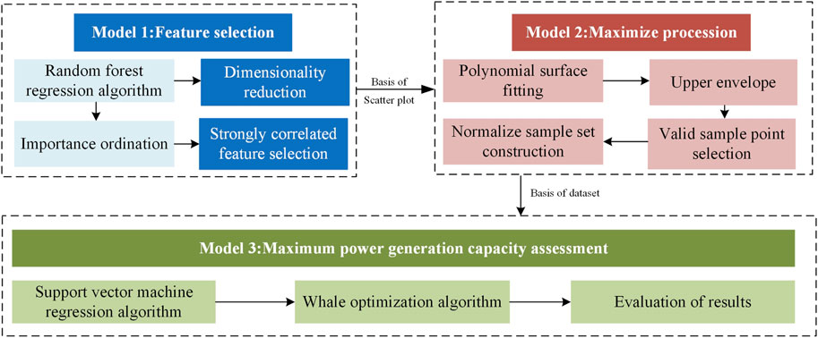
FIGURE 1. Overall framework of the three models.
The innovation of this paper lies in the envelope analysis method based on polynomial surface iterative fitting, which constitutes the data pre-processing model based on polynomial fitting. In addition, this paper mainly uses the RF algorithm for data correlation analysis and the whale optimization support vector regression algorithm for sample prediction training. The specific analysis contents of each model are as follows:
(1) The feature selection model utilizes the RF algorithm to analyze the correlation of key variables that influence wind power generation capacity, such as meteorological equipment, and selects the two most significant correlation variables. Chuanjun et al. (2021) did not consider the wind power time-varying characteristics and complex nonlinear relationships as well as the utilization of a gradient boosting decision tree and artificial neural network supervised learning algorithms in the original correlation analysis to train the wind power model. A correlation analysis based on the importance of the influencing factors and the amount of bias dependence was proposed. The correlation characteristics of the temperature and power system load characteristics were obtained through physical relationships and Pearson’s correlation coefficient, aiming to determine the dynamic relationship between multifactorial variable quantities (Rui et al., 2015). Different from the linear correlation analysis method, the feature selection model in this paper uses the random forest algorithm to conduct the correlation analysis of influencing factors, taking into account both linear correlation and nonlinear correlation so that the correlation analysis is more comprehensive.
(2) The data pre-processing model is based on polynomial surface fitting to maximize and normalize the original dataset, aiming to build a more accurate learning sample set. Currently, most research on the maximum capacity of new energy power is based on maximum power point tracking. Le et al. (2023) implemented an overview of modern MPPT algorithms applied to permanent magnet synchronous generators in wind power conversion systems with MPPT methods based on speed convergence, efficiency, self-training, and complexity. Venkata et al. (2023) directly adopted solar panel technical parameters and proposed a new method of MPPT for photovoltaic (PV) panels based on an SVR machine. Unlike Venkata et al. (2023), which focused on analyzing the unique and complex operating mechanisms of PV panels, this study commences from the perspective of data, which can considerably avoid complex mechanism analysis. This model focuses on the maximization method, and studies on upper-envelope analysis are limited.
(3) The maximum generation capacity evaluation model utilizes the whale optimization algorithm (WOA) to improve the SVR machine and derive the correspondence between the input features and maximum generation output to improve the accuracy of the maximum generation capacity regression learning of wind power plants. In order to improve the evaluation effect of maximum power generation capacity based on SVR, this paper selects the whale optimization algorithm to optimize the parameters of SVR. In the field of power forecasting, there are many studies on the optimization of support vector machines that choose the whale optimization algorithm. YUE et al. (2020) showed that compared with particle swarm optimization (PSO) and genetic algorithm (GA), the introduction of WOA to optimize the parameters in SVR can greatly improve the prediction accuracy of the SVR model. WANG et al. (2022b) analyzed genetic algorithm, whale optimization algorithm, and improved whale optimization algorithm (IWOA) to optimize the parameters of SVR. Compared with GA, the optimization effect of WOA is greatly improved, but that of IWOA is not obvious and the operation time is greatly increased. Therefore, WOA is selected to optimize the training parameters of SVR when the maximum generation capacity is evaluated in this paper.
2 Key feature selection model based on random forest
RF key feature selection refers to the selection of the most effective features from multiple-source feature variables to reduce the dimensionality of a dataset (Chuanjun et al., 2021). To build a model to calculate the maximum new energy generation capacity, the reliability of historical data and completeness of the key parameters are crucial for the accuracy of the model, and the accuracy of features and data determines the upper limit of the prediction model performance (Rui et al., 2015). The validity of data is fundamental in data mining-related studies. Therefore, to improve the data quality of the model, a real dataset should be obtained and pre-processed to construct a valid sample set.
For the correlation analysis of the maximum wind power generation capacity, the required data type is part of the meteorological dynamic information and historical operation information. First, the historical equipment data of wind turbines are obtained from the wind farm supervisory control and data acquisition system (SCADA system) and sampled every 10 min. Then, the data information of the region where the wind turbine is located is obtained from the numerical weather forecast, and the resolution is set at 10 min. Before the numbers of leaf nodes and decision trees were determined, the multi-source dataset to be selected had seven key features: wind speed, wind direction, ambient temperature of the numerical weather forecast at the time of prediction, actual nacelle temperature, blade angle, wind angle, and power generation at the previous prediction moment. The forecast key feature set is listed in Supplementary Table S1. Thus, the RF key feature selection method is utilized to select the two features with the highest contribution rate to power prediction to achieve effective dimensionality reduction and facilitate the subsequent improvement of the learning algorithm performance.
2.1 The random forest algorithm
RF is a novel machine learning (ML) algorithm. Feature selection utilizing the RF method is a step in data pre-processing that involves training the RF regression prediction model. This study utilizes the CART decision tree as a weightless sampling method for weak learners. The CART decision tree is a classifier that utilizes multiple decision trees to train and integrate prediction of samples, update the weight sampling technique to construct multiple samples by randomly sampling data from the original samples, and use a random splitting technique of nodes for each resampled sample to construct multiple decision trees. Finally, it combines the multiple decision trees and obtains the final prediction result by voting (Guo and Wen, 2016).
The RF model is an integrated algorithm based on decision trees. The classical algorithms for decision tree learning are ID3, C4.5, and CART. The CART algorithm was primarily utilized in this model. The algorithm utilizes the Gini index to measure the uncertainty of data and determines the optimal classification features to ensure that all attributes of the sample dataset are utilized and completely classified, which is a greedy algorithm. Suppose sample set A is divided into
However, the decision tree algorithm does not consider the correlation between feature attributes; the single-decision approach is easy to overfit, and information is gained from features with more types of values. Multiple decision trees can be combined to build an RF model to overcome the disadvantages of the decision tree algorithm (Ahmadi et al., 2020). The RF algorithm utilizes a sampling method without weights or put-backs to enhance the accuracy of the learning algorithm. Training sample data are sampled to generate n subsets of samples that are assigned to n decision trees. RF does not restrict the growth of each decision tree and does not require pruning of the decision trees.
A decision tree can be generated by utilizing two major steps: processing of divisible nodes and random selection of the desired variables to improve accuracy. When decision trees are generated via node splitting, each decision tree selects attributes and generates branches according to the splitting rule. In this study, the CART algorithm was selected as the base splitter of RF, and the Gini index was utilized as the node-splitting rule. To reduce the correlation of each decision tree and improve the classification accuracy when node splitting of decision trees is performed, several of these attributes are selected for comparison by randomly selecting variables (forest-RI) (Ziqiang et al., 2022).
The RF algorithm generates many decision trees through the aforementioned steps, and these decision trees constitute the RF. n randomly constructed decision trees are utilized to classify a test sample, and the classification results of each randomly constructed decision tree are aggregated to derive the final classification result according to the voting method.
2.2 Key feature selection algorithm based on random forest
The key feature selection model utilizes the RF algorithm to evaluate the importance of each feature. The importance score of each feature can be calculated depending on its use in different decision trees. The higher the score, the greater the influence of this feature on the prediction results. The RF feature selection principle can handle high-dimensional and sparse features, thereby avoiding conventional feature selection methods for dimensional disasters. Meanwhile, when the RF algorithm is utilized to analyze the correlation of feature variables, it analyzes from the perspective of linear correlation and nonlinear correlation of correlated factors. Furthermore, RF integrates multiple input attributes and is suitable for complex data; it is fast, efficient, and highly stable for processing sample data. Moreover, the model can achieve high classification accuracy and prediction capability without adjusting too many parameters.
In RF key feature selection,
Suppose n decision trees exist and n sample subsets are constructed, the importance of the ith feature can be calculated as follows:
Step 1. Initially, set n = 1 and construct a decision tree as
Step 2. Regression prediction is performed on the OOB dataset
Step 3. The value of the ith feature in
Step 4. Steps 1–3 are repeated for n = 2,3,4,…,N;
Step 5. The importance of the ith feature
3 Data pre-processing model based on polynomial fitting surfaces
This study mainly focuses on the data-driven statistical prediction model, which focuses on the maximum output of new energy rather than the real-time output prediction of new energy, which is also different from the existing power prediction method. There is no maximization processing in the existing power prediction technique, and the common method is to directly train and learn the acquired raw data after simple pre-processing, while this study requires complex pre-processing of the acquired raw data, which is also the innovation of this study. In this research, data pre-processing mainly includes normalization processing and maximization processing. Before using the upper envelope surface method to select the maximum output, the key feature data need to be normalized to improve the accuracy and efficiency of the model.
3.1 Normalization process
Before the maximum wind power generation capacity is predicted and calculated, wind speed and temperature need to be normalized. The wind speed is (0,20) m/s, and the temperature is at (−20,40)
In the wind power maximum generation capacity calculation model, wind speed and temperature can be normalized by analogy with existing wind power forecasts. The normalization method of both variables is the same, and the method is the ratio of the current value of the variable to the historical maximum value. The normalization formula is expressed as follows:
Here,
3.2 Maximization process
This study proposes maximization processing for the maximum generation capacity assessment requirement, with the ability to screen valid data points. We propose a processing method to screen the maximum wind power output points by utilizing polynomial surface-fitting iterations to construct valid datasets for subsequent ML. Because the dataset with zero power was not meaningful for the maximum generation capacity assessment, the dataset with zero output was removed in this study to improve the iteration efficiency.
After feature selection, wind speed and temperature were utilized as input feature variables to draw a three-dimensional (3D) scatterplot of wind speed, temperature, and exit force. After acquiring the 3D scatterplot, as shown in Figure 2, the maximization process to construct the upper envelope by analogy with the 2D planar scatterplot and the idea of polynomial plane fitting applied to the 3D scatterplot to construct the upper envelope surface were carried out. In the linear regression treatment, a fitted surface was constructed for the 3D scatterplot, a polynomial surface was fitted to the scatter points, and the scatter points in the upper part of the constructed surface were screened to form a set. This operation was repeated for the scattered points in this set, and the surface constructed by the scattered points in the final set approximated the best upper envelope of the original scattered-point plot in several iterations. The specific steps are as follows:
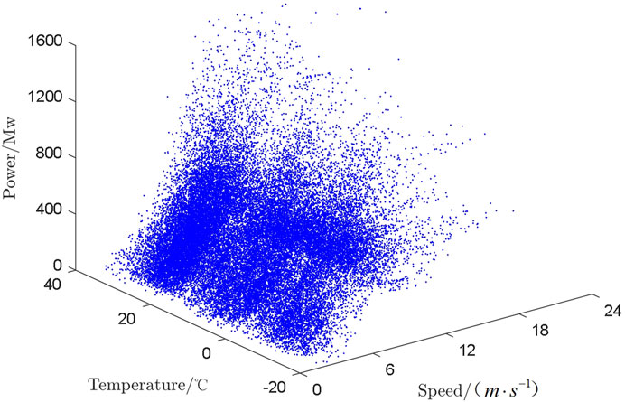
FIGURE 2. Wind speed-temperature-power scatterplot.
Step 1. A 3D scatterplot is constructed with wind speed, temperature, and historical wind power as the x-axis, y-axis, and z-axis, respectively, and the original dataset is recorded as set
Step 2. By utilizing a polynomial approach for surface fitting, a surface-fitting function
Step3. In the (i−1) iteration, let the scatter be
Step 4. The iteration is terminated when it satisfies the condition
4 Maximum generation capacity evaluation model based on whale optimization support vector regression
4.1 Maximum generation capacity assessment algorithm
4.1.1 Support vector regression machine
The basic principle of SVR is to calculate the decision function in the feature space for a given training sample set, followed by a regression prediction utilizing the decision function (Venkata et al., 2023). For linearly indistinguishable problems, mapping of the sample data to a high-dimensional feature space by utilizing a kernel function and determination of the linear decision function in the high-dimensional feature space outperform other ML algorithms when the number of samples is small. In this study, after maximization, the number of samples was 5%–10% of the original data; therefore, the SVR algorithm was adopted (Ghali et al., 2022).
The sample training set is
Let the decision function of the sample set in the feature space be
Here,
where
where
where
SVR is a supervised ML method with a complete theoretical foundation; however, different parameter selections have a direct impact on the prediction accuracy and generalization ability of the model (Shakul et al., 2022). The penalty parameter C and kernel function parameters must be optimized in the SVR model. Therefore, we utilize the whale algorithm to optimize the SVR parameters.
4.1.2 Optimization of SVR parameters based on the whale optimization algorithm
The WOA is a global search algorithm derived from the unique bubble-net feeding behavior of humpback whales (CHEN et al., 2023). The algorithm achieves an optimized search by simulating whales contracting the envelope, spiraling to update the hunt, and searching for prey (Samita et al., 2022). The whale optimization algorithm is simple in principle, easy to be programmed, and has better solution accuracy and convergence speed with fewer parameters. Optimizing the parameters of the new energy maximum power generation capacity evaluation model based on SVR can improve the evaluation accuracy of the prediction results. The WOA optimizes the parameters of SVR by optimizing the penalty coefficient C and kernel function parameters as well as utilizing the training error of SVR as the individual fitness value. The WOA–SVR parameter optimization process is shown in Figure 3.
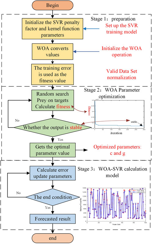
FIGURE 3. Flowchart of the support regression machine algorithm optimized by the whale algorithm.
When the whale algorithm was not utilized, the two parameters were not randomly selected; however, the plane where the two parameters are generally obtained was empirically divided into equally spaced grids, and the parameters on the grid nodes were selected individually for SVR training. After all nodes were trained, the training error was compared, and the parameter value with the smallest training error was selected as the optimal parameter value. The aforementioned optimization algorithm is simple, and the existence of the optimal parameters on the grid nodes is not guaranteed. Therefore, the optimization algorithm is too rough, and the parameters may only be local optimal solutions in the grid. In contrast, the WOA is a heuristic algorithm for optimal search, which is characterized by simple operation, simple structure, easy implementation, and few adjustable parameters in the parameter optimization process, which can considerably avoid being caught in the local optimal solution.
In the WOA, the whale perceives the prey, swims in the direction of the optimal whale individual, and identifies the location of the prey surrounding it (Chu et al., 2022). The mathematical model is shown in Eq. 8:
where t is the current number of generations sent,
where a is the control parameter,
When the whale obtains the position information of the prey, it spirals continuously to approach the prey, with the prey’s position as the center. To encircle and spirally approach the prey, the whale is judged by probability p whether to contract the encircling or spirally update the position. When p < 0.5, the encirclement contraction method is executed; when p > 0.5, the spiral update method is executed. The mathematical model is shown in Eq. 11:
where
The whale algorithm utilizes the size of A as the basis to determine whether to execute a random search for prey. When A < 1, the method of encircling the prey is executed; when A ≥ 1, the whale cannot obtain valid clues, and the random search for the prey is utilized to obtain valid information regarding the prey:
where
4.2 Evaluation indexes
The correlation coefficient and root-mean-square error were the main evaluation indexes in this study. The model performance is improved, and the prediction accuracy is higher when the correlation coefficient is closer to 1 and the root-mean-square error (Ermse) is small (ZHANG et al., 2022).
4.2.1 Correlation coefficient
The correlation coefficient r reflects the correlation between the predicted maximum power generation and the fluctuation trend of the measured maximum power generation in the envelope of the 3D scatterplot.
where
4.2.2 Root-mean-square error
Ermse is the most commonly utilized error evaluation metric to measure the superiority of ML.
where
5 Computer simulations and discussion
5.1 Random forest feature selection algorithm analysis
5.1.1 Optimization of the number of decision trees and leaf nodes
The number of decision trees and leaf nodes must be determined before selecting the key feature variables using the RF algorithm. The error of the RF model decreased with an increase in the number of decision trees; however, the computation time and the number of learning cycles of the model increased, and overfitting occurred, thus decreasing the generalization ability. Thus, the number of decision trees and leaf nodes must be optimized to ensure the effectiveness of the RF algorithm. Generally, the minimum number of leaf nodes is set to five for decision tree training in regression problems (Breiman, 2001).
In this example, the minimum leaf node parameters are assumed to be 5, 10, 20, 50, 100, 200, and 500 to determine the best decision tree and leaf node parameters for the same training set. The OOB error of different leaf nodes changed rapidly and slowly with an increase in the number of decision trees during the training process, and the fastest and most stable OOB error was selected. The number of leaf nodes with the smallest error was selected as the optimal leaf node parameter, and the minimum number of decision trees when the error was stable was selected as the optimal number of decision trees in the training model to optimize the training speed and reduce the training cost. The variation curves of the error results with the number of OOB decision trees for different leaf node parameters are shown in Figure 4.
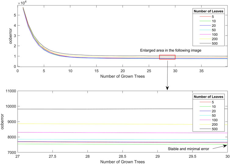
FIGURE 4. Variation curve of OOB error and the number of decision trees.
As shown in Figure 4, in the decreasing error phase with the number of decisions, the error-decreasing speeds of choosing the number of leaf nodes as 10 and 20 were similar, and both can be chosen as the parameter with the fastest error-decreasing speed. From a comprehensive consideration of the error stabilization phase curve, the minimum OOB error can be achieved when the number of leaf nodes is 10, whereas the stabilization error is larger when the number of leaf nodes is 20. Meanwhile, for the selection of the number of decision trees, the error remained stable after the decision trees reached 30, which is evident from the curve changes. Based on the aforementioned considerations, the optimal number of leaf nodes was set to 10, and the number of decision trees for training was set to 30.
5.1.2 Key feature selection
Data from a wind farm in China for 2021 were analyzed as a case study, and 52,067 time points were selected to obtain the corresponding data. The seven key features of 52,067 time points in the sample set were utilized as input independent variables, and the actual output power of the current moment was utilized as the input dependent variable, trained in an RF model with minimum blade number 10 and decision tree number 30. The importance of the seven features was measured by utilizing the feature importance measure based on OOB data. The importance measurement results are shown in Figure 5.
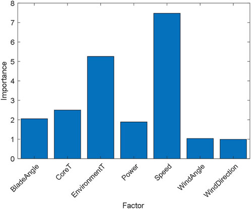
FIGURE 5. Histogram of feature importance measures.
As shown in Supplementary Table S2, the wind speed and environmental temperature significantly impact the actual power generation when utilizing the RF model for power generation prediction. Therefore, in the data pre-processing stage, to determine the maximum power generation boundary and predict the maximum power generation capacity, the two features of environmental temperature and wind speed were selected as data inputs to reduce data dimensionality, improve the prediction calculation efficiency, and avoid falling into the dimensional trap while retaining the features that significantly impact the predicted value to ensure the scientific accuracy and effectiveness of the prediction.
5.2 Analysis of the data pre-processing model
Data from a wind farm in China for 2021 were utilized as a case study, 52,067 time points were selected, and under each time point, three data points of wind speed, wind direction, and actual output power were available for this wind farm. A 3D right-angle coordinate system was constructed with wind speed as the x-axis, wind direction as the y-axis, and wind turbine historical real-time output as the z-axis. A 3D scatterplot of wind speed–wind direction–output of the wind turbine was drawn based on the obtained dataset. Meanwhile, the scatterplots in the original dataset were formed as a set of
A polynomial fit surface was constructed to determine the upper envelope; however, the upper envelope cannot be determined by performing a simple polynomial fit only once. To determine the target sample points, a polynomial fit surface was constructed several times by applying iterations. Suppose the iteration termination factor
After the first surface fit, as shown in Figure 6A, set
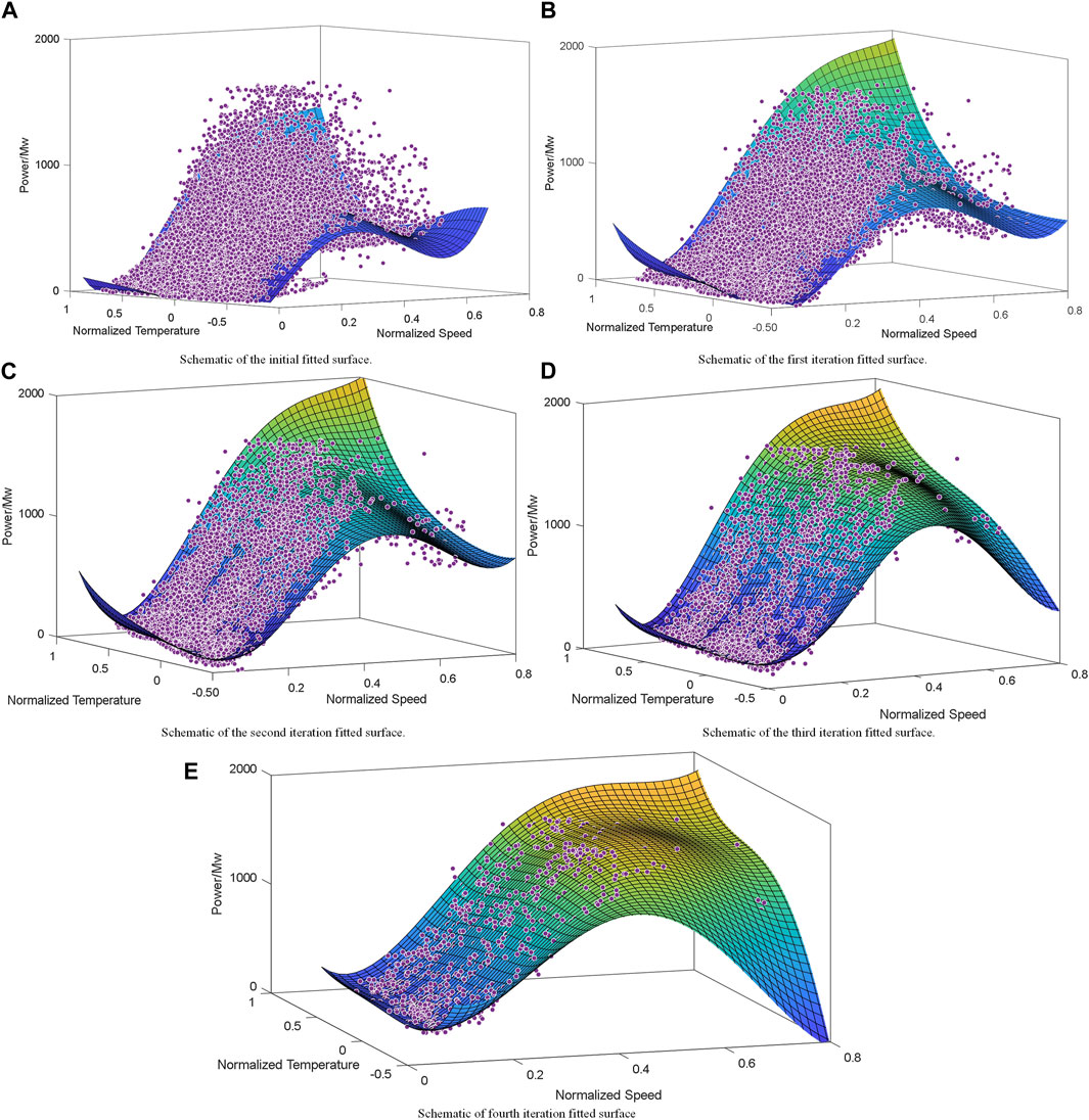
FIGURE 6. Schematic of the envelope construction process.
The results of the five polynomial surface-fitting constructions are shown in Figure 6. The iteration terminates when the difference in the number of elements in the target set between the two iterations is less than 2% of the original number of sample points for the first time, and the elements of the current iteration are considered valid sample points. As shown in Figure 6E, in the fourth iteration, the termination condition was satisfied for the first time, set
The polynomial fitted surface correlation coefficient formed as a result of the fourth iteration is shown in Supplementary Table S4. This polynomial, which was the basis for the screening of set
5.3 Analysis of the generation capacity boundary assessment model
To optimize the penalty coefficient C and kernel function parameters of SVR by utilizing the WOA, the population size was set to 20, and the iterations were calculated 300 times with the optimized values of both parameters ranging from 0.001 to 1,000. The individual whale position parameters in each iteration process were substituted into the SVR model for training, and the SVR training error was utilized as the fitness value of each individual whale. The minimum fitness value in the iteration was selected, and the whale position was updated for the next iteration. An adaptation curve of the minimum fitness value for each iteration with an increasing number of iterations was constructed, as shown in Figure 7. As the WOA optimization proceeded, the minimum fitness decreased gradually and converged to the optimal parameter point under the current parameter-taking range after nearly 100 iterations. In this example, the penalty factor and kernel function parameters were 6.6773 and 3.5954 after WOA optimization, respectively.

FIGURE 7. Adaptation curve graph.
The sample set was randomly divided into a training set and a test set according to a given ratio to test the model effects. The normalized wind speed values and temperature in the set were utilized as inputs, and the corresponding historical real-time wind farm output was utilized as the output. Before ML, the 429 datasets were randomly divided into 350 and 79 datasets by the program, and the randomly divided 350 and 79 datasets were utilized as the training set and test set to test the effect of the completed training ML model, respectively. To randomly assign the effective sample set of the experiment serial number
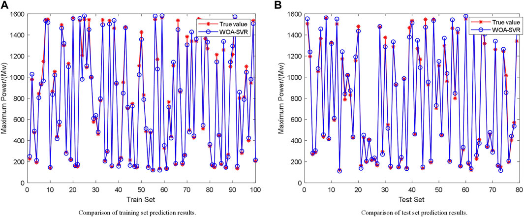
FIGURE 8. Comparison of WOA-SVR prediction results.
Based on the datasets within the training set, the model was trained using the WOA–SVR and unoptimized SVR algorithms, and the test set was validated, as shown in Figure 9. After optimization, Ermse was reduced from 0.055907 to 0.035662, and the correlation coefficient
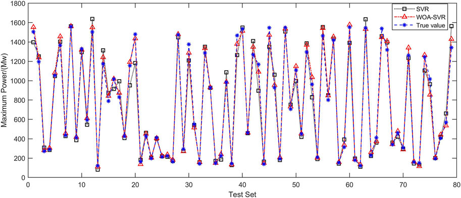
FIGURE 9. Comparison chart of test set prediction results.
Therefore, the WOA–SVR algorithm was more effective than the non-parameter-optimized SVR algorithm in predicting the maximum generation capacity. To analyze the power prediction result index, the Ermse and correlation coefficient were selected as measures, and the effective sample set was randomly divided into two parts, the training and test sets, and simulated thrice, that is,
From Supplementary Table S5, for the Ermse, the average error of the model constructed with the WOA–SVR algorithm was less than 3.3%, whereas that of the single SVR algorithm was over 5%; that is, the optimization of the whale algorithm decreased Ermse. For the squared correlation coefficient, the results of the three simulations of the WOA–SVR algorithm were over 0.99, whereas that of the single SVR algorithm was significantly lower than 0.97; that is, the correlation coefficient was closer to 1 owing to the WOA–SVR algorithm, which fully reflected the effectiveness of WOA–SVR parameter optimization.
6 Conclusion
This study proposed a polynomial surface fitting-based model to calculate and evaluate the maximum power generation capacity of new energy sources, which could be utilized to determine the available capacity of new energy sources and design a frequency stability control strategy to ensure the safe and economic operation of new energy power systems.
(1) A data-driven model was constructed, and the completeness and reliability of the data were crucial for the accuracy of the model calculation results. The utilization of RF feature selection for correlation analysis and effective screening of multi-source features could measure the nonlinear impact of changes in multiple influencing factors on the power generation capacity.
(2) The innovative step of the proposed model was based on the maximization analysis processing of key feature variables. Through polynomial surface-fitting iterative calculation, the upper envelope was constructed in the 3D scatterplot of the key feature variable—wind plant output—to achieve the maximization evaluation requirement.
(3) The WOA–SVR algorithm was utilized to predict the maximum power generation capacity of new energy sources, and a comparative analysis with the unoptimized SVR algorithm was conducted. The WOA–SVR algorithm was more effective and applicable.
The new energy maximum generation capacity assessment model was based on feature selection and maximization processing models, and the accuracy of the model influenced the assessment and analysis results. The data-driven model constructed in this study could be integrated with the maximum power tracking point of the physical model to analyze the size of the available FM capacity of new energy. The evaluation and analysis of the maximum power generation capacity in this study were completely based on historical data without relying on a physical model, which had a limited effect on the analysis of the sparse distribution of data points; thus, further studies involving a physical model are required.
Data availability statement
The original contributions presented in the study are included in the article/Supplementary Material; further inquiries can be directed to the corresponding author.
Author contributions
YH: Writing–original draft. HL: Writing–review and editing. YZ: Writing–review and editing. QC: Writing–review and editing. HC: Writing–review and editing. WC: Writing–review and editing.
Funding
The author(s) declare that no financial support was received for the research, authorship, and/or publication of this article.
Acknowledgments
This study was conducted at the School of Electrical and Information Engineering of Tianjin University, Tianjin, China.
Conflict of interest
Authors HL and QC were employed by State Grid Economic and Technological Research Institute Co., Ltd. Author WC was employed by State Grid Sichuan Economic Research Institute.
The remaining authors declare that the research was conducted in the absence of any commercial or financial relationships that could be construed as a potential conflict of interest.
The authors declare that this study received funding from the Science and Technology Project of the State Grid Corporation of China (No. 5100-202256014A-1-1-ZN). The funder had the following involvement in the study: data collection and analysis.
Publisher’s note
All claims expressed in this article are solely those of the authors and do not necessarily represent those of their affiliated organizations, or those of the publisher, the editors, and the reviewers. Any product that may be evaluated in this article, or claim that may be made by its manufacturer, is not guaranteed or endorsed by the publisher.
Supplementary material
The Supplementary Material for this article can be found online at: https://www.frontiersin.org/articles/10.3389/fenrg.2023.1323559/full#supplementary-material
References
Ahmadi, A., Nabipour, M., Mohammadi-Ivatloo, B., Amani, A. M., Rho, S., and Piran, M. J. (2020). Long-term wind power forecasting using tree-based learning algorithms. IEEE Access 8, 151511–151522. doi:10.1109/access.2020.3017442
Amir, M., and Zaheeruddin, H. A. (2022). Intelligent based hybrid renewable energy resources forecasting and real time power demand management system for resilient energy systems. Sci. Prog. 105 (4), 003685042211321. doi:10.1177/00368504221132144
Chen, B., Wang, J., Zhao, M., et al. (2023). Research on MPPT control of photovoltaic power generation system based on improved whale optimization algorithm. Proc. CSU-EPSA 35 (02), 19–26. doi:10.19635/j.cnki.csu-epsa.001057
Chu, Z., Chunlei, J., Lei, H., Ma, H., Nazir, M. S., and Peng, T. (2022). Evolutionary quantile regression gated recurrent unit network based on variational mode decomposition, improved whale optimization algorithm for probabilistic short-term wind speed prediction. Renew. Energy 197, 668–682. doi:10.1016/j.renene.2022.07.123
Chuanjun, P., Jianming, Y., and Yan, L. (2021). Correlation analysis of factors affecting wind power based on machine learning and Shapley value. IET Energy Syst. Integr. 3 (3), 227–237. doi:10.1049/esi2.12022
Ghali, Y., Sathyajith, M., and Leal, J. (2022). Power production forecast for distributed wind energy systems using support vector regression. Energy Sci. Eng. 10 (12), 4662–4673. doi:10.1002/ese3.1295
Guo, X., and Wen, Y. (2016). Data visualization research on monitoring data of wind turbines based on random forest. Electr. Meas. Instrum. 53 (22), 12–15+43.
Jiang, T., and Liu, Y. (2023). A short-term wind power prediction approach based on ensemble empirical mode decomposition and improved long short-term memory. Comput. Electr. Eng., 110. doi:10.1016/J.COMPELECENG.2023.108830
Kumar, V., Pal, Y., and Tripathi, M. M. (2019). A hybrid SVM-NARX based prediction method for Indian wind power sector. J. Statistics Manag. Syst. 22 (2), 363–378. doi:10.1080/09720510.2019.1580910
Le, X. C., Duong, M. Q., and Le, K. H. (2023). Review of the modern maximum power tracking algorithms for permanent magnet synchronous generator of wind power conversion systems. Energies 16 (1), 402. doi:10.3390/en16010402
Lin, Y., Cihang, Z., Yong, T., et al. (2019). Hierarchical model predictive control strategy based on dynamic active power dispatch for wind power cluster integration. IEEE Trans. Power Syst. 6 (34), 4617–4629. doi:10.1109/tpwrs.2019.2914277
Niu, D., and Ji, H. (2020). Quantitative analysis method for errors introduced by physical prediction model of wind power. Automation Electr. Power Syst. 44 (08), 57–65.
Ozkan, M. B., and Karagoz, P. (2019). Data mining-based upscaling approach for regional wind power forecasting: regional statistical hybrid wind power forecast technique (RegionalSHWIP). IEEE Access 7, 171790–171800. doi:10.1109/access.2019.2956203
Peng, X., Xiong, L., Wen, J., et al. (2016). A summary of the state of the art for short-term and ultra-short-term wind power prediction of regions. Proc. CSEE 36 (23), 6315–6326+6596. doi:10.13334/j.0258-8013.pcsee.161167
Qi, C., and Wang, X. (2021). Short-term prediction of offshore wind power considering wind direction and atmospheric stability. Power Syst. Technol. 45 (07), 2773–2780. doi:10.13335/j.1000-3673.pst.2020.1242
Rao, SNVB, Yellapragada, V. P. K., Padma, K., Pradeep, D. J., Reddy, C. P., Amir, M., et al. (2022). Day-ahead load demand forecasting in urban community cluster microgrids using machine learning methods. Energies 15 (17), 6124. doi:10.3390/en15176124
Rui, M. A., Zhou, X., Zhou, PENG, et al. (2015). Data mining on correlation feature of load characteristics statistical indexes considering temperature. Proc. CSEE 35 (1), 43–51. doi:10.13334/j.0258-8013.pcsee.2015.01.006
Samita, P., Prasad, B. P., and Prasad, D. D. (2022). Positional identification based whale optimization algorithm for dynamic thermal–wind–PV economic emission dispatch problem. Trans. Indian Natl. Acad. Eng. 7 (3), 977–994. doi:10.1007/s41403-022-00343-1
Shakul, S. H., Ramesh, R., Kannadasan, R., et al. (2022). A framework-based wind forecasting to assess wind potential with improved grey wolf optimization and support vector regression. Sustainability 14 (7), 4235. doi:10.3390/SU14074235
Shang, Yi, Gao, Z., Han, W., et al. (2020). Ultra-short-term wind power forecasting based on RF and GRU network. China Sci. 15 (09), 987–992.
Sun, Q., Yang, L., and Zhang, H. (2018). Smart energy-Applications and prospects of artificial intelligence technology in power system. Control Decis. 33 (05), 938–949. doi:10.13195/j.kzyjc.2017.1632
Venkata, M. P., Meyyappan, S., and RamaKoteswaraRao., A. (2023). Support vector regression machine learning based maximum power point tracking for solar photovoltaic systems. Int. J. Electr. Comput. Eng. Syst. 14 (1), 100–108. doi:10.32985/ijeces.14.1.11
Wang, K., Li, P., Tang, H., et al. (2021). Short term wind power prediction based on improved particle swarm optimization BP network. Ind. Control Comput. 34 (11), 119–121.
Wang, S., Chen, S., Chen, B., et al. (2014). Power model of wind power farm considering smoothing effect. J. South China Univ. Technol. Nat. Sci. Ed. 42 (04), 34–39.
Wang, Y., Liu, E., and Huang, Y. (2022a). An ultra-short-term wind power prediction method based on CNN-LSTM-lightGBM combination. Sci. Technol. Eng. 22 (36), 16067–16074.
Wang, T., Li, S., Huang, Y., and Sipeng, H. A. O. (2022b). Wind power forecast based on IWOA -svm. Mach. Electron. 40 (05), 9–12.
Wen, PENG, Xie, F., and Zhang, Z. (2019). Short-term wind power forecasting algorithm based on similar time periods clustering. Proc. CSU-EPSA 31 (10), 81–87. doi:10.19635/j.cnki.csu-epsa.000167
Xiang, X., Zhao, D., Wang, J., et al. (2012). A hybrid wind power prediction approach based on ARIMA and double BP neural network. Electr. Power Sci. Eng. 28 (12), 50–55.
Yan, J., Gao, X., Liu, Y., Han, S., Li, L., Ma, X., et al. (2015). Adaptabilities of three mainstream short-term wind power forecasting methods. J. Renew. Sustain. Energy 7 (5), 053101. doi:10.1063/1.4929957
Yue, X., Peng, X., and Lin, Li (2020). Short-term wind power forecasting based on whales optimization algorithm and support vector machine. Proc. CSU-EPSA 32 (02), 146–150.
Zeng, B., Xu, H., Zou, J., et al. (2013). A novel grey theory based short-term wind power prediction. Int. J. Appl. Math. Statistics™ 49 (19), 238–247.
Zhang, G., Ren, J., Zeng, Y., Liu, F., Wang, S., and Jia, H. (2023). Security assessment method for inertia and frequency stability of high proportional renewable energy system. Int. J. Electr. Power and Energy Syst. 153, 109309. doi:10.1016/j.ijepes.2023.109309
Zhang, Y., Ziyang, P. I., Zhu, R., et al. (2022). Wind power prediction based on WOA-BiLSTM neural network. Electr. Eng. 10, 28–31. doi:10.19768/j.cnki.dgjs.2022.10.009
Zhao, Y., Zhuo, L. I., Lin, Y. E., et al. (2023). A very short-term adaptive wind power forecasting method based on spatio-temporal correlation. Power Syst. Prot. Control 51 (06), 94–105. doi:10.19783/j.cnki.pspc.220850
Keywords: random forest, feature selection, polynomial fitting surfaces, whale optimization, support vector regression machine
Citation: Hu Y, Li H, Zeng Y, Chen Q, Cao H and Chen W (2023) Polynomial surface-fitting evaluation of new energy maximum power generation capacity based on random forest association analysis and support vector regression. Front. Energy Res. 11:1323559. doi: 10.3389/fenrg.2023.1323559
Received: 18 October 2023; Accepted: 30 November 2023;
Published: 21 December 2023.
Edited by:
Bilal Taghezouit, Renewable Energy Development Center, AlgeriaReviewed by:
Minh Quan Duong, The University of Danang, VietnamMohammad Amir, Indian Institutes of Technology (IIT), India
Copyright © 2023 Hu, Li, Zeng, Chen, Cao and Chen. This is an open-access article distributed under the terms of the Creative Commons Attribution License (CC BY). The use, distribution or reproduction in other forums is permitted, provided the original author(s) and the copyright owner(s) are credited and that the original publication in this journal is cited, in accordance with accepted academic practice. No use, distribution or reproduction is permitted which does not comply with these terms.
*Correspondence: Yuan Zeng, emVuZ3l1YW5AdGp1LmVkdS5jbg==