Generator condition monitoring method based on SAE and multi-source data fusion

With the increasing number of units involved in power system regulation and the increasing proportion of industrial load, a single data source has been unable to meet the accuracy requirements of online monitoring of unit conditions in the new power system. Based on the stacked autoencoder (SAE) network, combined with multi-source data fusion technology and adaptive threshold, a generator condition monitoring method is proposed. First, a SCADA–PMU data fusion method based on the weighted D–S evidence theory is proposed. Second, the auto-coding technology is introduced to build a stacked self-coding deep learning network model, extract the deep features of the training dataset, and build a generator fault detection model. Finally, by smoothing the reconstruction error and combining it with the trend change in the state monitoring quantity detected by the adaptive threshold, the fault judgment is realized. The simulation results show that, compared with the traditional method based on a single data source, the proposed method has higher robustness and accuracy, thus effectively improving the refinement level of generator condition monitoring.

1 Introduction

As one of the core components of the power plant, the generator set maintains high speed for a long time and runs continuously in multi-coupling fields such as machine, electricity, grid, and heat. With the increasing number of units involved in regulation and the increasing proportion of industrial load, abnormal parameters or control strategies (Zhu et al., 2018; Wang and Chen, 2020) are found in some units during operation. If the parameter errors are not found in time and the dynamic characteristics of the generator are grasped, the conventional system regulation strategy may have negative effects, such as unit reverse regulation and deviation between actual power output and issued instructions, under system disturbances, such as system faults and system joint debugging processes. In severe cases, the disturbance range of the system may be enlarged, and the generator oscillation and other events may occur, which may lead to system safety problems. Therefore, higher requirements (Li, 2015; Wei et al., 2021) are put forward for online monitoring and fault diagnosis technology of generator sets.

Data-driven methodologies and physical model-based methods can be used to diagnose generator faults. Li H. M. et al. (2010) built the heat conduction model of each part of the generator based on the finite analysis method and simulated the temperature to realize the condition monitoring of the generator. However, the process of modeling and solving physical models is complex, and it is difficult to consider all influencing factors. Once the model is built, it is difficult to modify, and it is not practical in practical engineering application.

In recent years, some progress in the research on generator condition monitoring based on data-driven has been made. Sun et al. (2012) proposed an SVM method based on particle swarm optimization for vibration fault monitoring of generator sets. Zare and Ayati (2021) established a multi-channel convolution neural network model, which can be used for fault monitoring of various units. Ren et al. (2019) used variational mode decomposition and transfer learning to monitor faults. However, most data-driven model training needs a large number of historical known fault samples, so the demand for fault data is high. However, in practice, it is difficult to collect all types of fault samples, which brings some difficulties (Li D. et al., 2010) to the application of this type of algorithm.

A stacked autoencoder (SAE) is an efficient algorithm of deep learning, which only reconstructs the normal operation data, reduces the dependence on fault data, and is suitable for fault monitoring of small data. Zhao et al. (2018) and Zhao et al. (2019) realized fault monitoring of wind turbines through the SAE deep learning network based on sample data in the SCADA system. However, with the increasing number of units involved in regulation and the increasing proportion of industrial load in the power system, a single data source can no longer meet the accuracy requirements of online monitoring of unit status (Jiang et al., 2017). Under system disturbances, such as system fault and system joint debugging, SCADA and PMU record the fluctuation data of each unit in the network. SCADA and PMU have their own advantages and disadvantages. In order to realize their complementary advantages, it is necessary to integrate their monitoring data (Huang et al., 1999; Huang and Jia, 2017).

At present, most of the methods for fault identification in generator sets are to artificially select a certain monitoring parameter to set a fixed early warning threshold (Fang et al., 2021) according to historical experience. Chen et al. (2020) analyzed and calculated the contribution degree of each state parameter to the overrun of the monitoring index on the SAE model and then determined the threshold of the monitoring index under the normal operation of the unit. Xing (2021) calculated the absolute value of the average value of each state parameter by the sliding window and determined the product of its maximum value and sensitivity coefficient as the threshold value to monitor the state. However, the standard of the normal working state of the generator set is changing all the time, and the traditional method of judging the abnormal performance index of the equipment by a fixed threshold has its limitations, which can easily lead to misjudgment and missed judgment (Tian et al., 2021).

In view of this, this paper proposes a generator condition monitoring method based on the SAE network, which combines multi-source data fusion technology with the adaptive threshold. First, a SCADA–PMU data fusion technique based on the notion of weighted D–S evidence is suggested. Then, automatic coding technology is introduced to build a stacked self-coding deep learning network model, extract the depth characteristics of the training dataset, and build a generator condition monitoring model. Finally, combined with the adaptive threshold, the running state of the generator is monitored. The simulation results based on real-world examples demonstrate the great accuracy and robustness of the suggested strategy.

The main contributions of this paper are as follows: this paper uses SCADA–PMU fusion data to monitor the generator condition. Compared with a single data source, it solves the problems caused by the long sampling period of SCADA data and the single type of PMU data and effectively improves the accuracy and robustness of generator condition monitoring. The adaptive threshold suggested in this study resolves the issues of alarm latency brought on by a too-high threshold and false alarms brought on by a too-low threshold and effectively improves the refinement level of generator condition monitoring.

2 Multi-source data fusion technology

In this study, the identical data types gathered by SCADA and PMU are combined, the data from each device are synchronized, the data are then combined using the D–S evidence theory, and the decision-making outcomes are analyzed as a result. Figure 1 depicts the data fusion decision model.

FIGURE 1

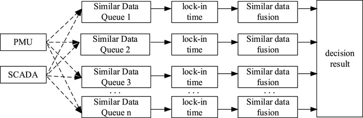
FIGURE 1. Data fusion decision model.

2.1 Determining the reference time

For the fusion of timescaled SCADA data and timescaled PMU data, time synchronization must be achieved first. The measurement time is relatively short and can be considered as both stationary. The usual method for measuring the temporal synchronization relationship of mixed measurement data is to obtain the correlation coefficient between the two.

${\rho }_{gw}\left(t_1,t_2-\tau \right)=\frac{c_{sw}\left(t_1,t_2-\tau \right)}{\sqrt{C_{ss}\left(t_1,t_2\right)c_{ww}\left(t_2-\tau ,t_2-\tau \right)}},(1)$

where ${\rho }_{gw}$ is the correlation coefficient of PMU measurement $Z_{\mathrm{w}}$ and SCADA measurement ${\mathrm{Z}}_s$; $t_1$ is the current SCADA measurement time (unknown); $t_2$ is the timescale of the current PMU data; $\tau$ is the time series of the current PMU; and $C$ is the cross-covariance function. Take $c_{sw}$ as an example, and it is expressed as follows:

$C_{\text{sw}}\left({\mathrm{t}}_1,{\mathrm{t}}_2-\tau \right)=R_{\text{sw}}\left({\mathrm{t}}_1,{\mathrm{t}}_2-\tau \right)-{\mu }_s{\mu }_w^{\mathrm{T}},(2)$

where ${\mu }_s$ and ${\mu }_w$ are the mean values of ${\mathrm{Z}}_s$ and $Z_w$ over a period of time, respectively. $R_{\text{sw}}$ is the correlation function of measuring ${\mathrm{Z}}_s$ and $Z_w$, and its expression is given as

$R_{\text{sw}}\left({\mathrm{t}}_1,{\mathrm{t}}_{\mathbf{2}}\right)=E\left\{{\mathrm{Z}}_s\left({\mathrm{t}}_1\right){\left[Z_w\left(t_2\right)\right]}^{\mathrm{T}}\right\},(3)$

${\rho }_{gw}\left(t_1,t_2-{\tau }_t{\rho }_{gw}\left(t_1,t_2-{\tau }_t\right)\right)=\max \left[{\rho }_{gw}\left(t_1,t_2-\tau \right)\right],(4)$

$t=t_2-\tau t,(5)$

where ${\rho }_{gw}\left(t_1,t_2-{\tau }_t\right)$ is a matrix of correlation coefficients; ${\tau }_t$ is the most relevant corresponding moment; and $t$ is the fusion data benchmark moment.

2.2 Determining a weight matrix of fusion data

The weight value is determined by the measurement data accuracy, and the data accuracy is determined by the measurement accuracy of the device and the reference time deviation:

$\epsilon =e_t+e_m,(6)$

where $\epsilon$ is the measurement data error; $e_t$ is the time synchronization error; and $e_m$ is the measurement error of the device.

The time synchronization error $e_t$ is determined by the reference time deviation and the rate of change of the measured quantity:

$e_t=k{t}_d,(7)$

where $k$ is the rate of change of the measurement and $t_d$ is the deviation between the measuring time and the reference time.

When the measurement error of the equipment is known, the time synchronization error must be determined first in order to derive the overall error. From the time synchronization of the timescale existing in the PMU measured data, it can be seen that the SCADA measured delay is regarded as obeying the following probability density:

$f\left(t_{\mathrm{d}}\right)=\frac{1}{{\sigma }_{t\sqrt{2\pi }}}{e}^{-{\left(t_d-t\right)}^2/\left(2{\sigma }_t^2\right)},(8)$

where ${\sigma }_t^2$ is the variance of $t_d$.

The overall error variance is stated as follows:

$E{\left[\epsilon \epsilon \right]}^T=E\left[e_{\mathrm{m}}{e}_{\mathrm{m}}^T\right]+k^{2}E\left[t_{\mathrm{d}}{t}_{\mathrm{d}}^T\right],(9)$

where $k^{2}E\left[t_{\mathrm{d}}{t}_{\mathrm{d}}^T\right]$ is the synchronization error variance ${\sigma }_t^2$.

As a result, the time synchronization-aware weight matrix can be expressed as follows:

$R^{-1}=\frac{1}{E{\left[\epsilon \epsilon \right]}^T}.(10)$

2.3 Data fusion technology based on the D–S evidence theory

In order to solve the problem of inconsistent sampling time between SCADA and PMU data, this paper finds samples similar to SCADA data in historical PMU data samples and uses the hot platform interpolation method to fill SCADA data.

This paper proposes a weighted D–S evidence theory-based data fusion approach. The difference between historical SCADA and PMU data is used to determine the weight of the SCADA data. The specific steps are as follows:

Step 1. Establish a recognition framework. The data samples to be fused are analyzed, and PMU and SCADA are taken as elements to form the recognition framework $\mathrm{\Theta }$ in the D–S evidence theory.

$\mathrm{\Theta }=\left\{{\theta }_1,{\theta }_2,\dots ,{\theta }_n\right\},(11)$

where $\theta$ is called an event or element of $\mathrm{\Theta }$. Their various combinations constitute the power set $2^{\mathrm{\Theta }}$, which is expressed as follows:

$2^{\mathrm{\Theta }}=\left\{\varnothing ,\left\{{\theta }_1\right\},\left\{{\theta }_2\right\},\dots ,\left\{{\theta }_n\right\}\right\}.(12)$

Step 2. Establish an initial trust allocation. In the recognition framework, the basic probability distribution function $m$ is obtained according to the data samples of the same category in the proposition.

$\left\{\begin{array}{c}m\left(\varnothing \right)=0,\\ {\displaystyle \sum _{A\subseteq \mathrm{\Theta }}}m\left(A\right)=1.\end{array}\right.(13)$

The basic probability number of event A is referred to as $m\left(A\right)$ in the formula, and it represents how much confidence is placed in A.

Step 3. According to the causal relationship, calculate the trust degree $m$ of all propositions. The trust degree of each proposition in the recognition framework is built using the reliability function and likelihood function of the D–S evidence theory. The degree of trust of a proposition is equal to the sum $Bel$ of the initial degree of trust of evidence in each of its premises.

$Bel\left(A\right)={\displaystyle \sum _{B\subseteq A}}m\left(B\right),(14)$

where $Bel\left(A\right)$ represents the degree of trust in the event A.

Step 4. Evidence synthesis. The information offered by various sources of evidence is combined using the D–S evidence theory, and the confidence level of each statement is calculated. The synthesis rules are shown in Formula 16:

$m\left(A\right)=\left\{\begin{array}{c}\frac{{\displaystyle \sum _{A^{\prime }\cap B_j=A}}{m}_1\left(A_i\right)m_2\left(B_j\right)}{1-K}\\ 0\end{array}\right.,(15)$

where $A$ and $B$ represent SCADA and PMU, respectively. $i$ and $j$ represent specific feature data in SCADA and PMU data, and the coefficient $\frac{1}{1-K}$ represents the normalized constant.

Step 5. Data fusion. Finally, the trust degrees of SCADA and PMU propositions are taken as weights, and the final fusion data $M$ is obtained by weighting them.

$M_i=m\left(A\right)A_i+\left[1-m\left(A\right)\right]B_i.(16)$

3 Stacked self-coding network

3.1 Self-encoder

A self-coding network consists of two visible layers of $d$ nodes and a hidden layer of $h$ nodes, as shown in Figure 2.

FIGURE 2

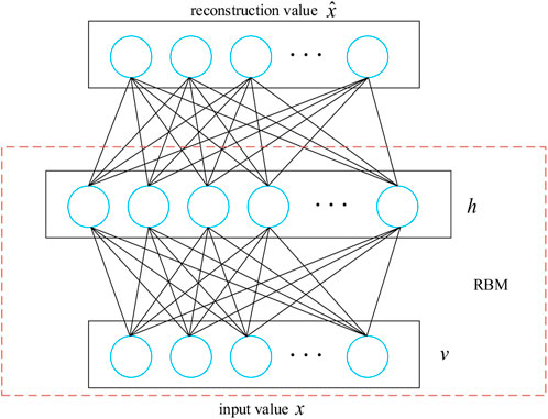
FIGURE 2. Self-coding network model structure.

In the model training process, input $x$ is encoded through the hidden layer to obtain $y$. The model then converts the encoded $y$ into a set of outputs through the decoder. The output layer is also considered the reconstruction of the input because the input and output layers both have the same number of nodes, designated as $\widehat{x}$ and having the same physical meaning as $x$. The reconstruction process can be expressed as

$y=f\left(W_{y}x+a\right),(17)$

$\widehat{x}=f\left(W_{z}x+b\right),(18)$

$f\left(x\right)=\frac{1}{1+{\mathrm{e}}^{-x}},(19)$

where $W_y$ and $W_z$ are the weights of the encoding and decoding processes, respectively; unit biases of the intermediate and output layers are represented by $a$ and $b$, respectively; and $f\left(\right)$ is the activation function. Therefore, in the training process, it is necessary to adjust the following parameters: $\theta$ = [$W,a,b$].

The objective function of the model is given as

$E=\underset{W,a,b}{\mathrm{arg\hspace{0.17em}min}}\left(c\left(x,\widehat{x}\right)\right),(20)$

where $\widehat{x}$ depends on parameter $\theta$ and $c\left(x,\widehat{x}\right)$ represents error $E$.

The basic structure of the self-encoder is a restricted Boltzmann machine (RBM), in which the nodes of the input and hidden layers can only take 0 or 1, that is, (v, h) $\in$ {0,1}. According to the Gibbs distribution, the joint distribution of the unit nodes can be obtained as

$P\left(v,h\right)=\frac{1}{z}{e}^{h^{T}Wv+b^{T}h+a^{T}v},(21)$

where $z$ is the normalized constant.

The conditional probability distribution of the unit nodes in the RBM can be expressed as

$E\left(v,h\right)=-h^{T}Wv-b^{T}h-a^{T}v,(22)$

$P\left(v_i=1|h\right)=f\left(a_i+W_{y}h\right),(23)$

$P\left(h_j=1\mid v\right)=f\left(b_i+W_{z}v\right).(24)$

The structure learning of RBM aims to fit the input data to the maximum extent. The reconstruction error $R_e$ is used as an index to describe the fitting degree:

$R_e\left(x,\widehat{x}\right)={‖x-\widehat{x}‖}^2.(25)$

Equation 26 represents the loss function. In order to update the network parameter $\theta$, we need to minimize the global loss function by the gradient descent method, so as to obtain the optimal solution of parameter $\theta$.

$J_{AE}\left(\theta \right)=\frac{1}{N}{\displaystyle \sum _x}{R}_e\left(x,f\left(x\right)\right),(26)$

$W^{\left(k+1\right)}=W^{\left(k\right)}+\epsilon \frac{\partial J_{AE}\left(\theta \right)}{\partial W},(27)$

$a^{\left(k+1\right)}=a^{\left(k\right)}+\epsilon \frac{\partial J_{AE}\left(\theta \right)}{\partial a},(28)$

$b^{\left(k+1\right)}=b^{\left(k\right)}+\epsilon \frac{\partial J_{AE}\left(\theta \right)}{\partial b},(29)$

where $\epsilon$ is the initial learning rate.

3.2 Stacked self-coding network

The SAE model is trained according to the training dataset of generator condition monitoring. The procedure is to train a single RBM, use the hidden layer’s output as the input of the following level, and then train the network parameters of the following level step by step until the full self-coding network has been parameter trained. By connecting the input and hidden layers of several self-encoders, an SAE network model is formed, which can deeply mine the characteristics of generator state variable data. Figure 2 shows a typical SAE network structure.

In the training process, the condition monitoring data $x$ of the generator set without labels in the long-term normal operation state is used as the pre-training sample. The model parameter $\theta$ is trained by minimizing the reconstruction error $R_e$ so that the input data $x$ is as close as possible to the decoded reconstruction value $\widehat{x}$. The input $x$ of the SAE network model can be expressed as $x$ = [I_A, I_B, I_C, I_fd, U_A, U_B, U_C, P, Q, θ, T_e, W_m, f, Δf], where the symbols in the formula correspond to ABC three-phase current and voltage, excitation current, output active and reactive power, power angle, electromagnetic torque, generator speed, frequency, and frequency change.

The output of the hidden layer can be utilized as the input of the higher layer to extract deeper features after the network has been created. This is performed by extracting features from the data and storing them in the hidden layer. If the model can well reconstruct the output data into the initial input, the reconstructed value of the input is obtained, which means that the trained model parameters retain enough rich information characteristics of the input data because the input variables correspond to the output variables and have the same physical meaning. Self-coding networks are connected to form a deeper SAE model and minimize the loss of input information, so that the network can maintain the constant complexity of data.

3.3 Adaptive threshold settings

In order to deal with the dynamic non-stationary characteristics of the generator during operation, it is necessary to filter and smooth the reconstruction error $R_{\mathrm{e}i}$, as shown in Eqs 30, 31. The processed reconstruction error value can be used to calculate an adaptive threshold for detecting anomalies. The alarm threshold can be calculated by adding the noise value to the standard deviation of the original reconstruction error $\sigma$, as shown in Eq. 32a.

$X_t=c+{\epsilon }_t+{\displaystyle \sum _{i=1}^p}{\phi }_i{X}_{t-i}+{\displaystyle \sum _{j=1}^q}{\theta }_j{\epsilon }_{t-j},(30)$

$y\left(p\right)=\frac{1}{{\displaystyle \sum _{k=-i}^i}w\left(k\right)}\left({\displaystyle \sum _{k=-i}^i}x\left(p+k\right)w\left(k\right)\right),(31)$

$U\left(t\right)={R_{\mathrm{e}i}}^{\prime }\pm n\sigma ,(\mathrm{32a})$

where p and q are the autoregressive and moving average orders of the model; φ and θ are undetermined coefficients that are not zero; ε_t is the independent error term; X_t is a stationary, normal, and zero mean time-series; y(p)is the weighted average of point p, p = 3, 4,..., n-2; w(k)is the weighting function, where w(k) = 1/(ak2+1), with the adaptive factor a, a > 0, and an integer k; x(p + k) is the measured value at point p + k on a curve; $y_i$ represents the reconstruction error $R_{\mathrm{e}i}$; $k$ is the sampling length; $U\left(t\right)$ is the alarm threshold; ${R_{\mathrm{e}i}}^{\prime }$ is the current value of the reconstruction error after the smoothing process; and $n$ is taken as 3.

When the generator works abnormally, the characteristics of the reconstruction error distribution will change, resulting in the reconstruction error value falling outside the control range. When this trend changes beyond the preset threshold, the generator can be judged to be abnormal. In practice, the monitoring threshold is usually set high, and there may be lag in monitoring abnormal changes in parameters directly. Therefore, the adaptive threshold can be used to determine the fault of the generator.

$\left\{\begin{array}{cc}{R}_e>U\left(t\right),& \text{abnormal\hspace{0.17em}warning},\\ R_e\le U\left(t\right),& \text{normal}.\end{array}\right.(\mathrm{33a})$

4 Experiment and result analysis

4.1 Data acquisition and parameter setting

In this paper, the experimental verification is divided into simulation example and actual example. The simulation example is based on the simulation data of a 60-MW single-machine system constructed using Simulink to establish the sample set. In the actual example, the monitoring data of a 250-MW #1 generator in a real power plant in Yunnan in the past 2 years under normal conditions are selected to establish the training sample set. All the simulation experiments are programmed in the Python environment.

Based on the operation data of multiple generators under normal operating conditions for several years as the training dataset of the model, different hidden layers and initialization parameters of RBM were selected to construct the SAE network model. The reconstruction error of the network was analyzed and compared. It was found that the SAE model of the generator was set with four hidden layers, each with a unit count of 1000, 500, 250, and 50, respectively. When the parameters W, a, and b of the SAE model are initialized to a random smaller value that follows a Gaussian distribution, the initial learning rate ε is set to 0.1, and the network update rate is set to 0.001; this set of parameters can better preserve the information of the training dataset. Moreover, when verified with multiple sets of data samples, this set of parameters has good stability. Therefore, this article finally selected the optimal parameter that retains the least generator information loss as the basic parameter of the model to further train the SAE network. Taking into account the impact of the iteration period on training time, the iteration period for parameter tuning is selected as 200.

4.2 Analysis of simulation results

In order to test the usefulness and accuracy of the abnormal state monitoring method of the generator based on data fusion, this study replicates the normal operation of the generator by increasing or decreasing the load.

Two faults are, respectively, set to simulate the method’s efficacy and correctness to carry out simulation verification:

Fault 1. Overload operation of the generator. The system is continuously connected to the load until the generator is overloaded at the 300th time point.

Fault 2. Generator three-phase short circuit. During the system, the load is increased or decreased to simulate the working condition under normal operation until the three-phase short-circuit fault occurs at the 400th time point.

In order to verify the robustness of this method, three methods are used to monitor the fault condition:

Method 1. Condition monitoring method based on SCADA–PMU fusion data and fixed threshold (Zhao et al., 2018).

Method 2. Condition monitoring method based on single SCADA data and adaptive threshold (Zhao et al., 2019).

Method 3. Condition monitoring method based on single PMU data and adaptive threshold.

Method 4. Condition monitoring method based on SCADA–PMU fusion data and adaptive threshold.

4.2.1 Simulation results of the data fusion method

In this paper, PMU and SCADA are regarded as elements in the recognition frame $\mathrm{\Theta }$, which are denoted as $\mathrm{\Theta }=\left\{A,B\right\}$. The importance of shared features of PMU and SCADA in input $x$ = [ I_A, I_B, I_C, U_A, U_B, U_C, P, Q, θ, W_m, f] of the SAE network model is taken as the trust degree in the D–S evidence theory, as shown in Table 1.

TABLE 1

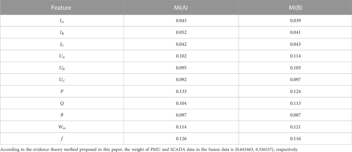
TABLE 1. Distribution of feature confidence.

4.2.2 Validity analysis of the adaptive threshold

This research simulates fault 1 using Methods 1 and 4 to determine the efficacy of the adaptive threshold. The simulation results are shown in Figure 3.

FIGURE 3

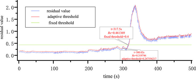
FIGURE 3. Simulation results of fault 1 by Methods 1 and 4.

Figure 3 shows that the monitoring variable $R_e$ starts to increase at 200 s, deviating from the original steady trend, and the load demand has approached the rated power of the generator at this time. When $R_e$ crosses the adaptive threshold at 300.02 s, a warning is issued. Approximately 10 s later, $R_e$ crosses again and remains above the adaptive threshold, thus judging that there is a fault. However, because the threshold value is generally set high in practice, the fixed threshold only sends an early warning signal at 317.5 s. The simulation results of Methods 1 and 4 for fault 2 are shown in Figure 4.

FIGURE 4

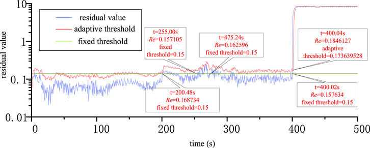
FIGURE 4. Simulation results of fault 2 for Methods 1 and 4.

Figure 4 shows that the monitoring variable $R_e$ begins to increase at 200 s, breaking away from the steady trend. The reason is that after 200 s, the load is randomly increased or decreased every 20 s to simulate the adjustment instruction of the AGC system to generator peak shaving. At 400.04 s, $R_e$ crosses and peaks above the adaptive threshold; the fault is judged, and an early warning signal is issued. Because the fixed threshold is set according to the normal operation of the generator in the previous 200 s, although the warning signal is generated 0.02 s earlier than the adaptive threshold when the generator is short-circuited, many false alarms are generated in the process of peak regulation of the generator. Compared with the fixed threshold, the adaptive threshold proposed in this paper solves the false alarm caused by a too-low threshold and the alarm hysteresis caused by a too-high threshold and has good robustness and accuracy.

4.2.3 Robustness analysis of fused data

The reconstruction effect of the stacked self-coding network is assessed in this paper using the mean absolute error and the root mean square error, with the mean absolute error and root mean square error being expressed as shown in Eqs 32b, 33b, respectively:

$\text{MAE}=\frac{{\displaystyle \sum _{i=1}^m}\left|y_i-x_i\right|}{m},(\mathrm{32b})$

$\text{RMSD}\sqrt{\frac{{\displaystyle \sum _{i=1}^m}{\left(y_i-x_i\right)}^2}{m},}(\mathrm{33b})$

where $x_i$ is the actual value of the multidimensional state variable of the ith sample, $y_i$ is the multidimensional state variable reconstruction residual of the ith sample, and $m$ is the sample number of the test dataset.

The stacking self-coding network proposed in this paper is used to simulate and verify the normal working condition of fault 1 by using Methods 2, 3, and 4, respectively, and the distribution of reconstruction residuals under the normal working condition of the model is shown in Figure 5.

FIGURE 5

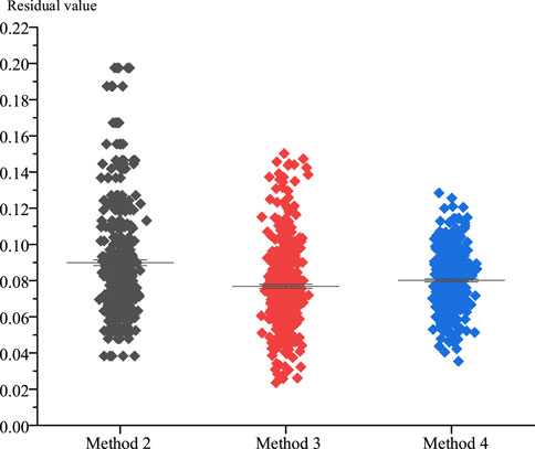
FIGURE 5. Distribution of residual values of the three methods.

Figure 5 shows that when Method 4 is used to train the model, the highest residual value is the smallest and the model residual value distribution is the closest. The reconstructed residual error results of the model under all working conditions are shown in Table 2.

TABLE 2

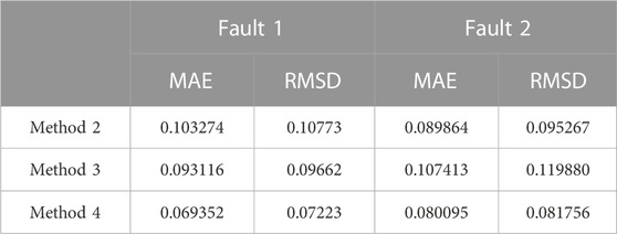
TABLE 2. Residual error results of model reconstruction.

As can be seen from comparing the simulation results in Table 2, the reconstruction effect of the model is best when using Method 4, and it is more resilient to the disturbance of time-varying working conditions. The average absolute error and root mean square error of the model are the smallest when using Method 4 to train the model.

4.2.4 Accuracy analysis of fusion data

The simulation results of fault 1 using Methods 2, 3, and 4 and the difference in distribution of its threshold and residual values are shown in Figures 6, 7, respectively.

FIGURE 6

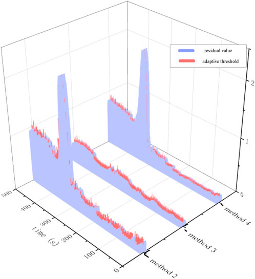
FIGURE 6. Simulation results of fault 1.

FIGURE 7

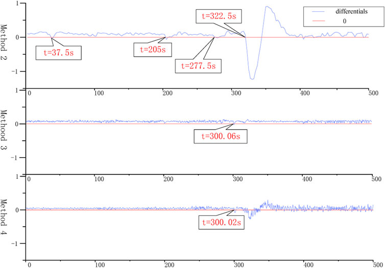
FIGURE 7. Difference between the threshold and residual values of fault 1.

Figure 7 shows the difference between the threshold value and the residual value. When the difference value drops below 0, it means that $R_e$ crosses the line and sends out a signal. It can be clearly seen from the figure that due to the limitation of SCADA data sampling step size, the warning time for $R_e$ to cross the threshold in Method 2 is 322.5 s, which is approximately 20 s slower than that in the other two methods. At the same time, the false alarms appeared at 37.5 s, 205 s, and 277.5 s in Method 2. Method 3 is also affected by the lack of PMU monitoring data, and $R_e$ is generally small. After the warning is issued at 300.06 s, $R_e$ falls back below the threshold after 0.04 s, and the response to the fault is not obvious enough, and there may be no alarm in the face of a gradual fault. Method 4 not only has no false alarm but also has the fastest warning time among the three methods, which shows that the reconstruction effect of Method 4 is the best, and the accuracy of disturbance under time-varying working conditions is better than the other two methods.

The alarm time and relative error of faults 1 and 2 simulated by Methods 2, 3, and 4 are shown in Table 3.

TABLE 3

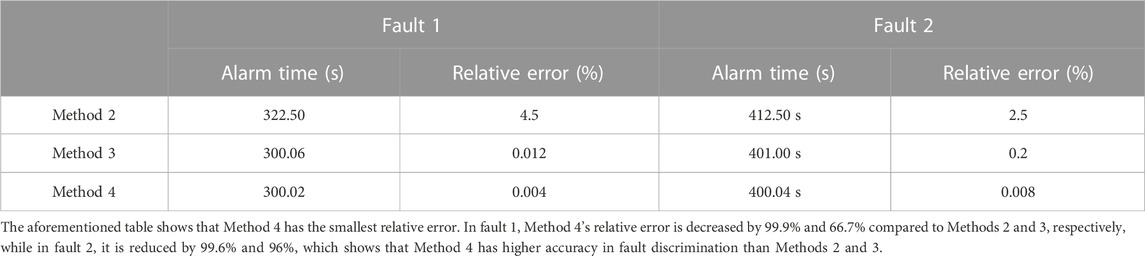
TABLE 3. Time for the residual value to cross the threshold.

4.3 Actual example

The fault case of #1 generator is that the load slip occurs at 10:14:57 on a certain day, then the output of #1, #2, #3, #4, and #5 generators in the power plant decreases, and the output of #1 ∼ #5 units decreases to 0 after approximately 48.55 s.

The operation fusion data of the #1 unit in a period of time before and after the failure is used for the test, and the simulation results are shown in Figure 8.

FIGURE 8

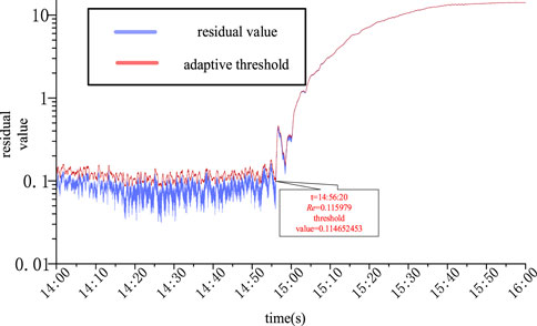
FIGURE 8. Simulation results of the #1 unit.

It can be seen from the simulation results that the monitoring variable $R_e$ suddenly increases at 10: 14: 56: 20 ms, crosses the threshold, and gives an early warning but falls back to the threshold after approximately 0.4 s. Finally, at 14 min and 59 s, it crosses again and remains above the threshold. At this time, it is determined that a fault has occurred and an early warning signal is sent out. It can be found that the method can send out the abnormal warning earlier, and the effectiveness and applicability of the method are verified by combining with the actual fault cases.

When the unit is in normal operation, the generator is in a state of dynamic balance; there is an internal relationship between the monitoring variables, and the trend change remains relatively stable. When an anomaly occurs, the long-term stable relationship is destroyed, and the monitoring quantity reflecting the overall state will deviate from the original trend. Through the examination of the generator of unit #1’s experimental findings, it can be verified that the fault breaks the relationship between the parameters, resulting in a change of trend of $R_e$.

This paper not only improves the monitoring threshold of the generator abnormal condition but also fully considers the influence of data structure on the monitoring model. Therefore, the monitoring scheme obtained has higher robustness and accuracy than the traditional methods.

5 Conclusion

For the research on the generator condition monitoring method, this paper proposes a generator condition monitoring method based on the SAE network, which combines multi-source data fusion technology and adaptive threshold. The proposed method’s effectiveness is confirmed by the actual fault scenario, which also serves the goal of the generator condition monitoring.

In this paper, the data of SCADA and PMU are fused to extract the internal relationship of multiple fused data parameters of the generator, and the abnormal state of the generator is judged by combining with the SAE network. Aiming at the sampling difference between SCADA and PMU data, a new data fusion method and adaptive threshold based on the D–S evidence theory is proposed in this paper, and it is combined with the SAE network to monitor the operation status of the generator. The simulation results demonstrate that the suggested method has more robustness and accuracy than the conventional method and can actually improve the refinement level of generator condition monitoring by realizing gradual failure prediction.

Data availability statement

The original contributions presented in the study are included in the article/Supplementary Material; further inquiries can be directed to the corresponding author.

Author contributions

CX: conceptualization, validation, writing–original draft, and writing–review and editing. XX: conceptualization and writing–review and editing. XH: methodology and writing–review and editing. ML: validation and writing–review and editing.

Funding

The authors declare that no financial support was received for the research, authorship, and/or publication of this article.

Conflict of interest

Authors CX, XX, XH, and ML were employed by the Electric Power Research Institute of Yunnan Power Grid Co., Ltd.

Publisher’s note

All claims expressed in this article are solely those of the authors and do not necessarily represent those of their affiliated organizations, or those of the publisher, the editors, and the reviewers. Any product that may be evaluated in this article, or claim that may be made by its manufacturer, is not guaranteed or endorsed by the publisher.

References

Chen, J., Jian, Li, Chen, W., and Sun, P. (2020). Anomaly detection method for wind turbine generator condition based on sliding window and multiple SNR stack de-noising self-coding. Electrotech. Trans. 35 (02), 346–358. doi:10.19595/j.cnki.1000-6753.tces.181577

CrossRef Full Text | Google Scholar

Fang, Y., Tang, S., Gu, B., Dai, S., and Ye, X. (2021). Research on data fusion technology based on binary bit missing identification and improved D-S evidence theory. Chin. J. Electr. Eng. 16 (03), 184–191.

Google Scholar

Huang, S., and Jia, W. (2017). A new method for locating stator ground fault of large turbogenerator. Power Syst. Prot. Control 45 (09), 35–40.

Google Scholar

Huang, Y., Tao, Y., Zhou, J., and Su, D. (1999). Application of D-S evidence theory in multi-sensor data fusion. J. Nanjing Univ. Aeronautics Astronautics 1999 (02), 57–62.

Google Scholar

Jiang, G., He, H., Xie, P., and Tang, Y. (2017). Stacked multilevel-denoising autoencoders: a new representation learning approach for wind turbine gearbox fault diagnosis. IEEE Trans. Instrum. Meas. 66 (9), 2391–2402. doi:10.1109/tim.2017.2698738

CrossRef Full Text | Google Scholar

Li, D., Rui, Li, and SunYuan Zhang, (2010). Data compatibility analysis of WAMS/SCADA hybrid measurement state estimation. Proc. Chin. Soc. Electr. Eng. 30 (16), 60–66.

Google Scholar

Li, H. M., Hou, J. Y., Li, J. Q., Wang, H. Y., and Xu, G. D. (2010). Multi-loop mathematical model of interturn short circuit in turbogenerator excitation winding. Proc. Chin. Soc. Electr. Eng. 30 (33), 58–64. doi:10.13334/j.0258-8013.pcsee.2010.33.009

CrossRef Full Text | Google Scholar

Li, J. (2015). Study on dynamic inter-turn short circuit fault location of turbogenerator excitation winding. Proc. Chin. Soc. Electr. Eng. 35 (07), 1775–1781. doi:10.13334/j.0258-8013.pcsee.2015.07.027

CrossRef Full Text | Google Scholar

Ren, H., Liu, W., and ShanWang, M. X. (2019). A new wind turbine health condition monitoring method based on VMD-MPE and feature-based transfer learning. Measurement 148, 106906. doi:10.1016/j.measurement.2019.106906

CrossRef Full Text | Google Scholar

Sun, H. C., Huang, C. M., and Huang, Y. C. (2012). Fault diagnosis of steam turbine-generator sets using an EPSO-based support vector classifier. IEEE Trans. Energy Convers. 28 (1), 164–171. doi:10.1109/tec.2012.2227747

CrossRef Full Text | Google Scholar

Tian, Ye, Xu, T., Yan, Li, Deng, X., and Wang, Y. (2021). Fault line detection in resonant grounding system based on reconstruction error and multi-scale cross sample entropy. Power Syst. Prot. Control 49 (13), 95–104. doi:10.19783/j.cnki.pspc.201061

CrossRef Full Text | Google Scholar

Wang, H., and Chen, Q. (2020). Transient stability assessment method based on cost-sensitive stacked variational autoencoders. Proc. Chin. Soc. Electr. Eng. 40 (07), 2213–2220. doi:10.13334/j.0258-8013.pcsee.182346

CrossRef Full Text | Google Scholar

Wei, S. R., Zhang, X., Fu, Y., Ren, H. H., and Ren, Z. X. (2021). Early fault warning and diagnosis of offshore doubly-fed wind turbine based on GRA-LSTM-Stacking model. Proc. Chin. Soc. Electr. Eng. 41 (07), 2373–2383. doi:10.13334/j.0258-8013.pcsee.200224

CrossRef Full Text | Google Scholar

Xing, Y. (2021). Research on key technologies of operation condition monitoring and health maintenance of wind turbine. Beijing: North China Electric Power University. doi:10.27140/d.cnki.ghbbu.2021.000150

CrossRef Full Text | Google Scholar

Zare, S., and Ayati, M. (2021). Simultaneous fault diagnosis of wind turbine using multichannel convolutional neural networks. ISA Trans. 108, 230–239. doi:10.1016/j.isatra.2020.08.021

PubMed Abstract | CrossRef Full Text | Google Scholar

Zhao, H., Yan, X., Wang, G., and Yin, X. (2019). Fault diagnosis of wind turbine generator based on deep self-coding network and XGBoost. Automation Electr. Power Syst. 43 (01), 81–86.

Google Scholar

Zhao, H. S., Liu, H. H., Liu, H. Y., and Lin, Y. K. (2018). Wind turbine generator condition monitoring and fault diagnosis based on stacked self-coding network. Automation Electr. Power Syst. 42 (11), 102–108.

Google Scholar

Zhu, Q., Chen, J., Li, H., Shi, D., Li, Y., and Duan, X. (2018). “Power system transient stability assessment based on stacked autoencoders,” in Proceedings of the Chinese society of electrical engineering. doi:10.13334/j.0258-8013.pcsee.170095

CrossRef Full Text | Google Scholar