 Yazeed Yasin Ghadi1
 Hossam Kotb2*
 Kareem M. Aboras2
 Mohammed Alqarni3
 Amr Yousef3,4
 Masoud Dashtdar5
 Abdulaziz Alanazi6
- 1Department of Computer Science and Software Engineering, Al Ain University, Abu Dhabi, United Arab Emirates
- 2Department of Electrical Power and Machines, Faculty of Engineering, Alexandria University, Alexandria, Egypt
- 3Electrical Engineering Department, University of Business and Technology, Jeddah, Saudi Arabia
- 4Engineering Mathematics Department, Faculty of Engineering, Alexandria University, Alexandria, Egypt
- 5Department of Electrical Engineering, Faculty of Sciences and Technologies Fez, Sidi Mohamed Ben Abdullah University, Fes, Morocco
- 6Department of Electrical Engineering, College of Engineering, Northern Border University, Arar, Saudi Arabia
A combined algorithm for reconfiguring and placement of energy storage systems, electric vehicles, and distributed generation (DG) in a distribution network is presented in this paper. The impact of this technique on increasing the network’s resilience during critical periods is investigated, as well as improvements in the network’s technical and economic characteristics. The three objective functions in this regard are the network losses, voltage profile, and running costs, which include the costs of purchasing electrical energy from the upstream network and the devices used, as well as the cost of load shedding. In addition, the impacts of the presence of DG on power flow and the modeling of the problem’s objective function are examined. To solve the problem of reconfiguration and placement of a multi-objective distribution feeder, a genetic algorithm (GA) and shuffled frog leaping algorithm (SFLA) hybrid algorithm is used. The proposed GA–SFLA algorithm is used to solve the problem with changes in its structure and its combination in three stages. Finally, the proposed method is implemented on the 33-bus distribution network. The simulation results show that the proposed method has an effective performance in improving the considered objective functions and by establishing a suitable fit between the different objective functions based on the three-dimensional Pareto front. Moreover, it introduced a more optimized architecture with lower loss, lower operating costs, and greater reliability compared to other optimization algorithms.
1 Introduction
In recent years, increasing penetration of distributed generation (DG) sources in distribution systems has improved various characteristics such as reliability and reduced losses. On the other hand, due to the uncertainty of DG sources, providing too much load using these technologies will cause problems such as instability. In this way, to increase the penetration of renewable energy sources, the role of other technologies in power systems has become more prominent. Energy storage systems (ESSs) are one of these efficient pieces of equipment in the network, which can increase the penetration of renewable resources in the network by taking advantage of their charging and discharging properties. On the other hand, ESSs are not the only devices capable of charging and discharging in the network, and the properties of electric vehicles (EVs) can be used to improve the characteristics of the system and its optimal use (Karthikeyan et al., 2018; Dashtdar et al., 2020; Dashtdar et al., 2022a; Nawaz et al., 2023). Like ESSs, EV batteries can be charged and discharged. Due to the low battery capacity, it is possible to show its effect by combining these devices in the network. In addition, due to the expansion of the use of smart grids, basic issues in power systems have become more important, among these issues are reconfiguration, increasing the resilience of the distribution network under critical conditions such as floods and storms. This issue has been examined from different perspectives. One of the most important indicators for improving resilience is reducing system load shedding. Therefore, changing the structure of the distribution network and adding up-to-date technologies according to the existing conditions can lead to the improvement in the overall performance of the system (Sharma et al., 2020; Shi et al., 2022; Sui et al., 2022).
Several studies have been carried out on the optimal placement of energy storage devices, DG, and optimal reconfiguration in the network. In these studies, various optimization methods have been used to determine decision variables. Daily reconfiguration is carried out to reduce losses and improve reliability, which was initially executed using classical methods, but the distribution network includes hundreds of switches, so it was not possible to consider all the existing configurations and check all of them by classical methods, which is why today smart methods are used. The genetic algorithm (GA) was utilized by Dashtdar et al. (2021a) for reconfiguration and optimal placement of UPQC in the distribution network. One of the operational goals of reconfiguration is to improve the load balance index, which was studied by Kahouli et al. (2021), simultaneously reducing losses and reliability as objective functions. A multi-objective approach for optimizing the stochastic reconfiguration problem in the presence of wind turbines (WTs) and fuel cells is provided in the work of Nikkhah and Rabiee (2019).
Connecting DG resources to distribution systems can have a positive or negative effect on network performance, which can include reducing losses, improving voltage profile, improving reliability, reducing environmental pollution, and postponing investment for network development. The presence of DG in the reconfiguration problem will cause changes in the way of power flow and determine the objective function, which is generally considered a cost function with the presence of DG. Each DG source’s cost function is regarded as a multiplier of the power generated by it. Using the quadratic function to calculate the power generation cost of DGs is more suitable because the calculated cost for power generation will be closer to reality (Arif et al., 2017; Hamida et al., 2018; Dashtdar et al., 2021b; Dashtdar et al., 2022b). The appropriate allocation of DGs in the distribution system is a problem of optimization with both discrete and continuous variables. Some researchers have used intelligent and evolutionary methods to find the optimal location of DGs. Rafi and Dhal, (2020a) presented a new strategy for the optimal allocation of DG in the distribution feeder to minimize losses and increase the voltage at the end of the feeder during peak load using a hybrid optimization technique. Reddy et al. (2018) presented a method based on an Ant Lion Optimization algorithm to optimize DG in radial distribution systems and minimize losses from the point of view of subscribers. Hassan et al. (2022) presented the nature-inspired optimization algorithm as well as the techno-economic pattern to determine the optimal size and location of DG in distribution systems. By examining the research in this field, we notice a new perspective called the combination of two reconfiguration problems at the same time as the optimal allocation of DG units. Mahboubi-Moghaddam et al. (2016) proposed the multi-objective reconfiguration of distribution network feeders, considering the operating cost, transition stability, and losses using the EGSA. In this article, the transient stability is calculated by using the critical clearing times index and considering the probability of fault occurrence in different locations. In the work of Sedighizadeh et al. (2017), using the imperialist competitive multi-objective algorithm based on fuzzy logic, optimal reconfiguration for distribution networks to improve simultaneous losses, Average Energy Not Supplied (AENS), the System Average Interruption Frequency Index (SAIFI), the System Average Interruption Duration Index (SAIDI), and the Average Service Unavailability Index (ASUI) is proposed. Hooshmand and Rabiee (2019) proposed multi-objective energy management, considering the effects of reconfiguration, renewable resources, demand response, and energy storage. The proposed model simultaneously minimizes the cost of purchasing energy and unsupplied energy by determining the optimal location of renewable resources, storage devices, and demand response. Truong Anh et al. (2018) first addressed the placement and optimal size of the DG using the runner root algorithm and then performed the reconfiguration of the distribution network in the presence of the DG to reduce losses. Siahbalaee et al. (2019) presented a method for reconfiguration in the presence of DG, with the aim of minimum losses, minimum number of switches, and minimum voltage deviation of buses using the improved shuffled frog leaping algorithm (SFLA) and evaluated the effect of simultaneous reconfiguration and placement of DG in reducing losses and increasing the minimum level voltage. Teimourzadeh and Mohammadi-Ivatloo (2020) discussed optimization of the reconfiguration problem in the presence of DG to reduce losses and improve the voltage profile, in which different load levels were considered and the three-dimensional group search optimization (3D-GSO) method was used to solve the optimization problem. DG sources are modeled as negative load, and its effect on power flow is considered as voltage constraints. So far, meta-heuristic algorithms with various efficiency and accuracy and with different objective functions have been presented for the reconfiguration and placement problem of DG such as GA (Saonerkar and Bagde, 2014; Ajmal et al., 2021; Mahdavi et al., 2021), PSO (Jena and Chauhan, 2016; Saleh et al., 2018; Rafi and Dhal, 2020b), SFLA (Arandian et al., 2014; Azizivahed et al., 2017; Onlam et al., 2019), fuzzy (Sedighizadeh and Bakhtiary, 2016; Mohammadi et al., 2017; Hosseinimoghadam et al., 2020), and ABC (Jamian et al., 2014; Quadri and Bhowmick, 2020; Dashtdar et al., 2022c).
In recent years, there have been significant advancements in the field of multi-objective optimization of distribution networks with DG and EV placement. For instance, a study by Lotfi et al. (2020) presented a comprehensive analysis of the reconfiguration and optimization of distribution networks considering DG integration. The authors propose a methodology based on a multi-objective particle swarm optimization algorithm to minimize losses, improve voltage profile, and optimize the operation of DG units. Another relevant work in this field was conducted by Lotfi and Ghazi (2021). They investigated the integration of renewable energy sources, such as wind energy, into distribution networks. The authors propose a multi-objective optimization approach to simultaneously minimize power losses, improve voltage profile, and enhance the overall performance of the network. Furthermore, a recent study by Lotfi (2022) focused on the mutual effect of network reconfiguration and EV charging/discharging in distribution networks. The authors proposed a multi-objective optimization algorithm to optimize the placement of EV charging stations and the reconfiguration of the network, considering the impact on power losses, voltage profile, and EV charging/discharging. Additionally, the integration of ESSs is an essential aspect of the optimization of distribution networks. Lotfi (2020) investigated the impact of ESSs on the operation and performance of distribution networks with DG and EVs. The authors proposed a multi-objective optimization algorithm to minimize losses, improve voltage profile, and optimize the operation of energy storage systems in the network.
By including these references, we aim to provide a better understanding of the motivation behind our research, highlight the novelty of the proposed method, and demonstrate our awareness of relevant past works in the field. So, in this article, the problem of multi-objective optimization of reconfiguration of distribution networks with the placement of DG is discussed. The advantage of the proposed method in this article compared to previous research is the simultaneous combination of three objective functions including losses, voltage profile, and operating costs consisting of the costs of purchasing electrical energy from the upstream network and the devices used and the cost of load shedding. In this regard, a comprehensive mathematical model is presented to investigate the increasing penetration of wind energy as a renewable energy source in the network. In addition, in this model, the mutual effect of network reconfiguration on the number of vehicles being charged and discharged in the electric vehicle parking lot is investigated. The presented model is evaluated in 24 h under normal and critical conditions. In this way, assuming that the connection with the upstream network is interrupted during certain hours of the day, the amount of load interruption before and after the occurrence of the fault is obtained. Finally, according to the objective of the problem, from the point of view of the distribution company, in addition to minimizing the cost of purchasing electric energy from the upstream network and wind turbine owners and the cost of buying and selling energy to ESSs and EV parking, it also minimizes the cost of shedding controllable loads. Due to the complexity of solving the problem, therefore, the algorithm used must be accurate and efficient. In this article, an improved multi-objective hybrid algorithm combining GA and SFLA is presented by applying changes in their structure in three stages to minimize the cost of operation losses and improve the voltage profile. Finally, the differences and characteristics of the proposed strategy with references (Lotfi 2020; Lotfi et al., 2020; Lotfi and Ghazi, 2021; Lotfi, 2022) can be listed as follows:
• Optimal placement of PV, WT, ESS, and EV units in the network based on criteria F1, F2, and F3
• A detailed description of how to implement power flow in the network in the presence of DG units and display the power and voltage output of each network section
• Considering critical and real conditions such as failure and exit of some network lines, in addition to bringing the strategy closer to reality, reducing the costs of load shedding is evaluated in the problem
• Performance evaluation of the proposed hybrid GA–SFLA algorithm based on MID, diversity, NPS, and spacing criteria
This article is structured as follows: Section 2 defines the problem formulation and constraints. Section 3 presents the structure of the proposed hybrid GA–SFLA algorithm for solving the problem. Section 4 presents the simulation results and discussion. Finally, Section 5 summarizes the conclusion and future work.
2 Modeling and formulation of the placement and reconfiguration problem
Figure 1 shows the general problem space and solving method schematically. Here, three objective functions, including operating costs, losses, and total voltage deviations, are defined, and through simultaneous placement and reconfiguration, these objective functions based on the power flow are tried to be minimized with a subset of simple recursive equations. The algorithm implemented to solve the problem is a hybrid algorithm with a combination of GA and SFLA features, which are defined in three stages. The following section details how to model the units and formulate the problem along with the constraints. In this research, two types of DG sources, wind and solar, are used, and their output has uncertainty, so the important issue is how to model this uncertainty.
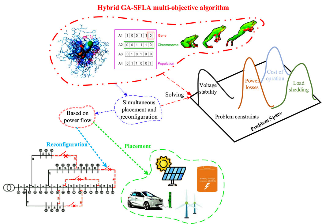
FIGURE 1. General space of the placement and reconfiguration problem.
2.1 Solar photovoltaic modeling
The amount of solar radiation and the ambient temperature are two critical factors that influence probability variations and behavior in photovoltaic (PV) power generation. The probability distribution function of these parameters can be generated using a variety of distribution functions, and the normal distribution function is utilized in this article to simulate the relevant parameters. After modeling solar radiation and ambient temperature with a probability distribution function, Eq. 1 is used to obtain the amount of PV generation power (Lotfi and Ghazi, 2021):
where the amount of solar radiation and ambient temperature under standard conditions are considered as GSTC = 1,000 W/m2 and Tr = 25°C, respectively. GING is the amount of solar radiation, Tc is the temperature around the cell, and kα is the temperature coefficient for the maximum power. Figure 2 shows the probability distribution function of PV generation power.
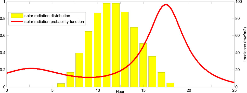
FIGURE 2. Probability power of the PV unit.
2.2 Wind turbine modeling
The wind speed is continually fluctuating. The average amount provided for a certain area cannot simply represent the amount of WT generation installed in that location. Probability distribution functions can be utilized to determine the abundance of wind speed in a region. The Weibull distribution is more commonly used in wind speed forecasting. The general relationship of a Weibull distribution with variable X with scale parameter λ and shape parameter K is expressed through the following equation (Lotfi, 2022):
For wind speed, we use the same probability distribution based on the following equation (Lotfi, 2022):
The parameters c and h represent scale and shape parameters for wind speed v, respectively. In this article, the values of c and h are considered as 9 and 2, respectively. The wind speed influences the output power of a WT, and there is a non-linear relationship between these two variables. The “power–speed” characteristic curve of WT, represented by Eq. 4 (Lotfi, 2022), illustrates the amount of active power produced by WT for varying wind speeds.
where vco, vr, and vci are the cut-out speed, rated speed, and cut-in speed, respectively. PWT,r is the rated speed of WT. Moreover, the probability distribution function of the WT-generating unit is depicted in Figure 3.
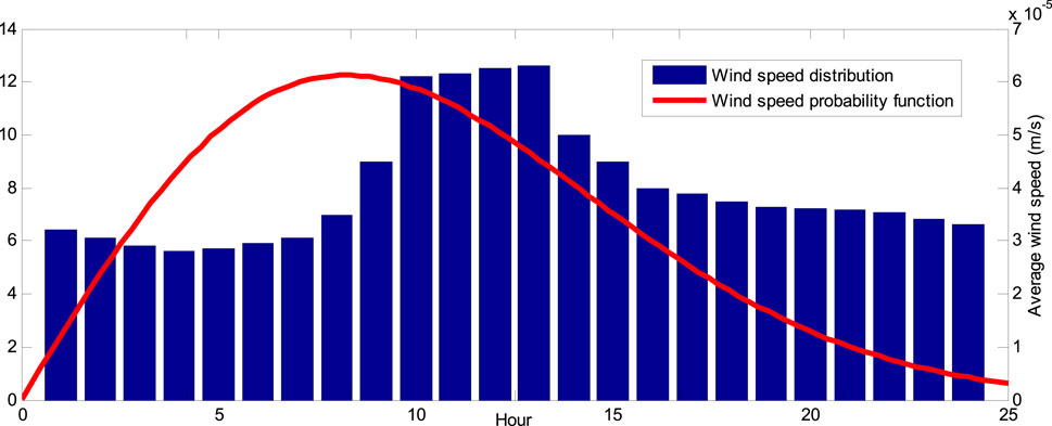
FIGURE 3. Probability power of the wind unit.
2.3 Modeling of the energy storage system
ESS is a system that stores energy at certain times and re-injects it into the system at other times. The performance of the ESS creates two important possibilities for the distribution network. One is the increase of inertia in the island network, which leads to the improvement of system stability, and the other is the activation of this system to improve economic performance. The operation of the ESS is based on the pricing shown in Figure 4, which shows the electricity price chart at different hours of the day based on the normalized monetary unit.
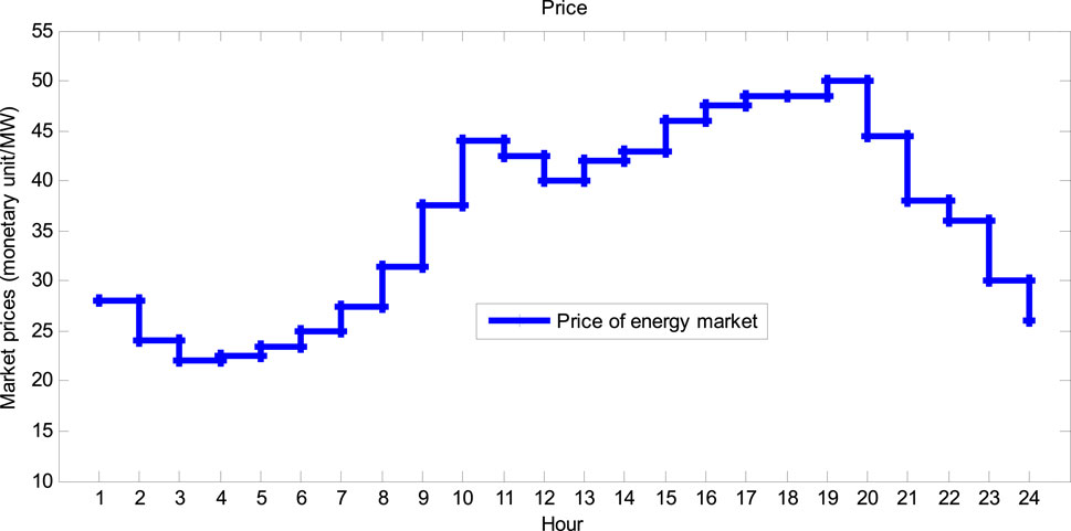
FIGURE 4. Electricity prices at different hours.
The considered protocol is in the following form of (Lotfi, 2020):
where EP(t) is the electricity price at time t, ESS(t) is the energy available in the energy storage system at time t, Δt is the smallest part of time equal to 1 h, and ch_rate and disch_rate are the charging and discharging rates of the ESS, respectively, which represent the power injected into the network during ESS operation.
2.4 Problem formulation
A multi-objective function is considered in this work which includes all costs of the distribution company and consists of three objectives. The first goal is to minimize the voltage deviations (VDs) of the entire network, which is defined as follows (Lotfi, 2020):
where Vit is the voltage of the ith bus at time t and Vide is the desired voltage of the ith bus equal to 1 p. u. Most losses in power systems are related to distribution networks. Reducing losses in distribution networks frees up system capacity, especially during load peak hours. Here, the second goal is to reduce the losses of the entire system, which is defined as follows (Lotfi, 2020):
where Ilt is the current of the lth line at time t and Rl is the resistance of the lth line of the network. One of the main goals in the design and development of distribution networks is to transfer electric power from distribution stations to subscribers at the lowest cost while maintaining network operation limits. Therefore, the third objective is to reduce the operating cost of the distribution network by considering DG, which is expressed as follows:
As shown in Eq. 8, the objective function F3 consists of different costs. Here, EP(t) is the price of electricity, the FRES function is related to the total cost of purchasing electrical energy from the upstream network and renewable wind and solar units, and the FEES function considers the costs of charging and discharging the battery so that when the ESS is charged, it can receive an amount from its owner and in case of discharge, an amount is paid to the ESS owner. The FEV function considers the parking costs of electric vehicles. In this model, each vehicle pays or receives an amount to the distribution company according to the amount of charging or discharging. The FVOLL function is related to the cost of load shedding. Naturally, due to the high cost of load interruption for the distribution company, there is no load interruption in normal situations, but in critical times due to the low availability of resources, there is a need to interrupt the load, where
To form the multi-objective function according to Eq. 10, the normalized form is used, where each function is normalized based on its maximum value, so the problem of the units of the functions not being the same is solved, and the functions also change in an almost equal interval. Therefore, in this article, the goal of minimizing Eq. 9 will be based on optimal reconfiguration and DG placement in the network, and this will be achieved under the condition that the constraints of the problem are met and network information can be extracted correctly. So, one of the important factors in this issue will be how to implement power flow in the distribution network because DG and reconfiguration have a direct effect on it, which will be mentioned in the next section.
2.5 Power flow equations
With the increasing effect of DG, the distribution network transforms from a passive to an active network. This requires changes in the analysis and distribution strategy. In the presence of DG, conventional power flow methods for the distribution system no longer have the desired performance, so it is necessary to make changes in these methods so that DGs, which are generally modeled as active photovoltaic (PV) or active–reactive power (PQ) nodes, can be included in power flow calculations. Therefore, DG units, which are controlled as PQ buses, are entered as loads with negative impedance in the power flow. Figure 5 shows a single-line diagram of a sample feeder with DG. In this case, the power flow used, which is generally forward–reverse power flow, is not complicated, but for DG units that are controlled as PV buses, the correct amount of reactive power injection produced by the unit must be determined. For this purpose, an initial guess for the amount of injected reactive power is considered, and the power flow of the network is similar to the previous state. Then, by comparing the relevant bus voltage with the desired value, the voltage difference is calculated, and the amount of injected or received reactive power is calculated to provide the desired voltage. Then, with the new value of the calculated reactive power, the power flow is performed again and the PV bus voltage difference is calculated, and this process continues until the desired constant voltage is reached. Finally, according to Figure 5, power flow equations can be defined as follows (Lotfi, 2020; Lotfi et al., 2020; Lotfi and Ghazi, 2021; Lotfi, 2022):
where Pk is the active power of bus k, Qk is the reactive power of bus k, Ploss,k is the loss of active power of bus k, Qloss,k is the loss of reactive power of bus k, PLk+1 is the active power consumption of bus k+1, QLk+1 is the reactive power consumption of bus k+1, Rk is the resistance of the communication line between bus k and k+1, Xk is the reactance of the communication line between bus k and k+1, Yk is the parallel admittance of bus k, and Vk is the voltage range of bus k.
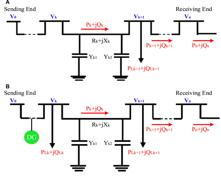
FIGURE 5. Single-line diagram of a sample feeder, (A) without DG and (B) with DG.
2.6 Problem constraints
The constraints of the problem consist of the reconfiguration limitations, power flow, maintenance of network characteristics, and the units used in it, which were pointed out. A graph is a radial network consisting of a tree without loops. To apply the reconfiguration limit for this condition, the number of network lines must be equal to the number of network buses minus one. Therefore, Eq. 14 must be valid, where Nbus is the number of network buses and Lr (i,j) is a binary variable indicating the state of the lines (Lotfi, 2020; Lotfi et al., 2020; Lotfi and Ghazi, 2021; Lotfi, 2022).
One of the main constraints is the consideration of power flow limits, in which various operating and physical limits of the network, such as network voltage limits, power passing through lines, and power injection to the network, are considered. In this article, in addition to the injection power from the upstream network, the power of WT, ESS units, and EV parking lots is considered. In addition, the power passing through the network lines is limited according to the network configuration (Lotfi, 2020; Lotfi et al., 2020; Lotfi and Ghazi, 2021; Lotfi, 2022).
Equations 15, 16 show active and reactive power balance relationships, respectively. Equation 17, 18 show the power flow in the grid lines. In Eqs 15, 16, the binary variable Lr (i,j) determines the disconnection and connection state of the lines and influences the power flow. Here, B (i,j) and G (i,j) are, respectively, the conductance and susceptance of the line between buses i and j.
According to Eqs 19, 20, 21, to comply with the limit of voltage and power passing through the lines, the apparent power passing through the lines must be within the specified range and the voltage of the buses must be within its permitted range. Furthermore, according to Eq. 22, the amount of interrupted load of each bus is determined according to the maximum bus load (Lotfi, 2020; Lotfi et al., 2020; Lotfi and Ghazi, 2021; Lotfi, 2022).
DG resources have generation limitations that are considered in this research. Eqs 23, 24 show the limit of active and reactive power of WT and Eq. 26 the limit of the active power of PV according to the available power of these sources every hour. In these relationships, the binary variables LWT (i) and LPV (i) determine the installation location of WT and PV units, respectively. According to Eqs 25, 26, 27, the number of WT and PV units that can be installed in the entire network is limited to a certain number, and this number can be affected by various factors. Here, eWT (t) and ePV (t) are the available power coefficients of WT and PV, respectively (Lotfi, 2020; Lotfi et al., 2020; Lotfi and Ghazi, 2021; Lotfi, 2022).
Eqs 28, 29 show the maximum charging and discharging power of ESS, respectively. In these relationships, the binary variables αESSch (i,t) and αESSdCh (i,t), respectively, determine the charge or discharge state of the battery, and according to Eq. 30, only one of them can be one in a specific hour. The number of ESSs that can be installed in the network is limited according to Eq. 31. In Eq. 32, SOCESS (i,t) represents the state of charge of ESS. Here, ηESSch (i,t) and ηESSdCh (i,t) are the charging and discharging efficiency of ESS and LESS(i), respectively, which determine the installation location of ESSs (Lotfi, 2020; Lotfi et al., 2020; Lotfi and Ghazi, 2021; Lotfi, 2022).
The limitations of the EV battery are modeled as the ESS battery. In addition to considering the charging and discharging state of the EV battery, the distance traveled by each EV is one of the elements of the energy function stored in the EVs (Lotfi, 2020; Lotfi et al., 2020; Lotfi and Ghazi, 2021; Lotfi, 2022).
Equation 33 shows the amount of energy of each EV. It should be noted that in this paper, it is assumed that there is a public parking lot in the network where EVs can be charged and discharged. The location of this parking lot is determined like other devices of the network. According to Eq. 36, the charging and discharging mode of an EV battery is defined according to binary variables αEVch (i,t) and αEVdch (i,t). In addition, PEVTR (i,v,t) is the power used to move the EV in the transportation system, which is obtained according to Eq. 37. δEV (v) is the consumption factor of EVs, and Eqs 38, 39 limit the type of each EV and the total number of EVs in the network, respectively. Here, LPL(i) determines the installation location of the EV charging station, and E0EV is the initial energy value of the EV.
3 The presented method for solving the problem based on a hybrid GA–SFLA multi-objective algorithm
One of the requirements in every reconfiguration problem is power flow. Irrespective of whether the reconfiguration problem is solved by mathematical methods or meta-heuristic methods, since restrictions such as the voltage of the nodes and the current of the branches must be observed, it needs power flow. Therefore, it is necessary to pay special attention to power flow in the distribution network. Another requirement of the reconfiguration problem is their solution method. Since almost all the mathematical methods that have been used so far in solving the reconfiguration problem are single-objective and used only to minimize the losses, and since in this article, the reconfiguration is supposed to be carried out simultaneously with the placement of the DG, and we also want to improve the losses and the voltage and operating cost, so mathematical modeling will be a complex issue. In this article, the hybrid GA–SFLA multi-objective algorithm is used in three stages based on answers in the form of a Pareto front to solve the problem.
3.1 Power flow in the distribution network
The power flows that are used in the reconfiguration issue should be written in a general way; that is, it should be effective for different configurations. Therefore, the algorithm must first have the ability to recognize the topology of the network, in such a way that it knows about all the branches of the network separately, from the slack bus to the end bus related to that branch. For example, if the network has four branches, two parameters must be defined, one of which shows the number of lines related to each branch, from the first line to the last line of the desired branch, and the other shows the number of buses in each branch, from the slack bus to the last bus of the subject branch. Before the topology detection algorithm is explained, it should be said that in any configuration that is given to the power flow program, all the information related to that configuration that is used in the power flow, including the active and reactive power of buses, the number of lines, the number of buses at both ends of each line, and the resistance and reactance of each line is given to the power flow. Suppose we want to get the network topology of Figure 6. According to the numbering of each line in Figure 6, Table 1 shows the beginning and end buses of each line.
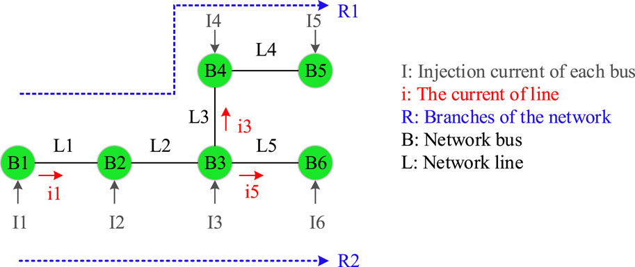
FIGURE 6. Sample distribution network for topology detection.
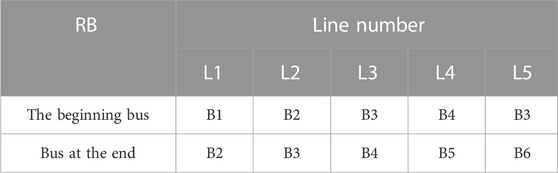
TABLE 1. Information about buses connected to lines.
The topology detection algorithm is as follows (Abul’Wafa, 2011):
• First, we need to know how many branches there are in each configuration. For this, we put all the beginning and end buses in the S vector. According to Table 1, the S vector will be as follows:
Buses that are repeated more than twice in the S vector show that a branch is coming out of those buses. The number of output branches is equal to the number of repetitions minus 2. For example, bus 3 (B3) was repeated three times, so one branch has been coming out from it. Here, the variable RB is defined, which represents the number of branches and is initially equal to 1.
• In this step, the RB variable is checked for each bus. Therefore, for each bus, the previous condition is checked and added to RB. As shown in Figure 6, only bus 3 is repeated more than twice, so the number of branches is equal to 2.
• The following process should now be carried out for as many as RBs:
(a) We start from the slack bus and set the desired variable B equal to 1.
(b) Then, we check from Table 1 that B contains the bus of the beginning or end of which line. If the bus was the beginning of the line, we set BB = B and B equal to the end bus, and if the bus was the end of the line, we again set BB = B and B equal to the first bus, and then, we store the number of the line in vector R and BB and B in vector N, and finally, we delete the column corresponding to that line.
(c) We continue the previous step until no line is found when checking B. It should be noted that if, during checking, we found that B was present in more than one line (that is, we reached nodes with several branches coming out of it, which is B3 here), we will choose one line at will; however, we must note that when we want to find the number of lines and buses of the next branches when we reach B3, the line selected in the previous step among the lines connected to B3 should not be chosen. The process of topology detection is as follows.
According to Table 2, after step (b) and checking line L1, column L1 is removed from Table 1 and the vectors R1 = [L1] and N1 = [B1, B2] are formed. Now, B = B2, and among the lines in Figure 6, only B2 exists in L2. After checking the L2 line, as shown in Table 3, vector R1 = [L1, L2] and N1 = [B1, B2, B2, B3] can be formed again.
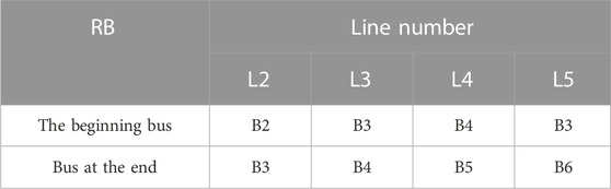
TABLE 2. The first step is to evaluate the lines.
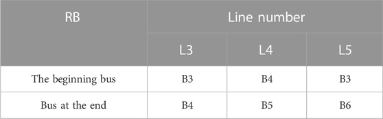
TABLE 3. The second step is to evaluate the lines.
Next is B = B3, and this bus is in lines L3 and L5. Therefore, a line, for example, line L5, is selected at will. After checking the L5 line, as shown in Table 4, vector R1 = [L1, L2, L5] and N1 = [B1, B2, B2, B3, B3, B6] can be formed again.
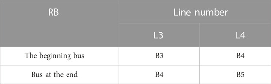
TABLE 4. The second step is to evaluate the lines.
B6 does not exist in any other line; thus, a branch is specified, and for the next branch, the same process starts from the beginning, with the difference that when it reaches bus B3, previously selected line L5 is no longer selected. Finally, the vectors R and N for all two branches become R1 = [L1, L2, L5], R2 = [L1, L2, L3, L4], N1 = [B1, B2, B3, B6], and N2 = [B1, B2, B3, B4, B5]. Therefore, by using the presented method, we can obtain the branches of any network configuration. As a result, by having branches, power flow calculations, including the calculation of TV and TI matrices (based on KVL and KCL), are implemented more easily.
According to Figure 6, the injected current in each bus can be obtained from Eq. 42, where Qi, Pi, and Vi are the reactive and active power of the load and the voltage of the ith bus, respectively. The negative sign is because the load is consumed in each bus, while this sign will be positive for the buses that DG is connected to.
The relationship between the injection current and branch current can be expressed as Eq. 43 based on the KCL law. These relationships can be defined based on the TI matrix as Eq. 44.
Similar to the previous case, the relationship between the branch current and bus voltage can be defined based on the KVL law, this time with the TV matrix. In Eq. 45, the method of calculating the bus voltage is defined, and in Eq. 46, the relationship between the voltage difference to the slack bus and the branch current is defined.
After calculating the DLF, first, all the buses are given an initial value of one. Then, the following process continues until the error is less than the desired value:
• According to the voltage and power of loads, the injection current of each bus is calculated.
• Using DLF, ΔV is calculated, and according to Eq. 47, the voltage of each bus is calculated:
• The amount of error in each step is calculated as follows:
Finally, the above algorithm is converged, and the voltages are calculated. Figure 7 summarizes the stages of the power flow algorithm.
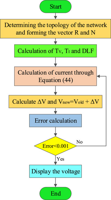
FIGURE 7. Flowchart of the power flow algorithm.
3.2 Hybrid GA–SFLA multi-objective algorithm
Although in the research conducted in the field of hybrid algorithms, GA is usually used as the basic algorithm, in this research, the concept of the SFLA is used as the basic algorithm. SFLA has a very good speed and also due to the grouping of the chromosomes, it will be possible to check all the chromosomes more easily during the execution of the program. However, the accuracy of the answers obtained in this algorithm is not enough, and this accuracy will decrease significantly in problems with a larger search space. GA is the most well-known meta-heuristic algorithm that has completely normal calculations and also has a high capability for changes in its operators. Therefore, it can be considered a suitable option for the auxiliary algorithm. In addition to using this algorithm, it is necessary to make changes to the operator of this algorithm to improve its efficiency of this algorithm. As shown in Figure 8, considering the multi-objective space of the problem, the hybrid GA–SFLA multi-objective algorithm based on the Pareto front is used to optimize the problem. Generating a complete Pareto front is one of the key components in various stages of multi-objective optimization. One of the most important features of the Pareto front is that one solution cannot be preferred over the other among the solutions, between two different solutions. A complete Pareto front gives the decision makers the authority to make the right choice according to the conditions of the project in terms of the project completion time, the costs of each activity, and finally, the minimum required. Considering that this research aims to optimize F1, F2, and F3 at the same time, therefore, we need to present a series of solutions with the same desirability among all the available solutions. For this, we use the Pareto front. As shown in Eq. 49, if any of the following conditions are met, the answer u will prevail over the answer v.
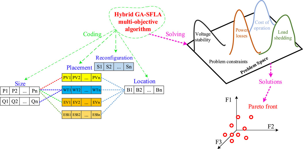
FIGURE 8. Optimization of the problem space based on the Pareto front.
Here, A and B mean F1 and F2, respectively. This comparison will be made for two factors, F1 and F3, as well as F2 and F3, to finally achieve a three-dimensional Pareto front. In the following discussion, the structure of the proposed algorithm will be presented. First, the structure of the improved SFLA will be introduced, and then, the method of combining it with GA will be presented in three steps.
3.2.1 Structure of the improved SFLA
Each frog in the SFLA technique indicates a potential solution to the problem. The initial population is separated into multiple independent groups using the assumed procedure with an equal number of frogs in each group. This algorithm employs two strategies for exploration based on this classification. The first strategy is called local search. As a result, by exchanging information, the frogs in each group increase their food position. The second technique involves information exchange between groups, in which the information gathered after each local search is compared between groups. To execute the algorithm, first, the algorithm’s initial parameters are specified, and then a random population with member POP is formed. The merit of each member is computed, and the population is divided into m groups, each of which has n members, after sorting the population in descending order. This classification should be made in such a way that members with the highest merit are represented in all groups. Then, a local search is performed for the mutation of the frogs with the lowest merit toward the frogs with the highest merit. This mutation is according to the following equation (Zhang et al., 2019):
where Xb and Xw denote the frogs with the best and worst solutions, respectively, D is the mutation value of the weakest frog toward the best member of the group, Dmax is the highest permissible limit for the frog mutation, and r is a random number between [0,1]. Based on Eq. 50, the direction of movement of the weakest frog toward the best frog is shown in Figure 9A. After applying the above changes, if the new frog has a better solution than the worst frog in the set, it will be replaced; otherwise, the same actions will be repeated by replacing Xg with Xb. If a more suitable solution cannot be found by applying the above changes, a solution will be generated randomly and will be replaced by the worst member of the group. This procedure is repeated for a set number of iterations until the algorithm’s completion conditions are finally met.
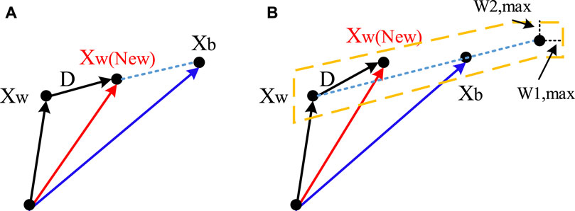
FIGURE 9. Mutation of the weakest frog to the best member of the group, (A) in the SFLA and (B) in the improved SFLA.
Here, two techniques are used to improve the performance of SFLA. In the first technique, by changing the mutation relation, the speed of the algorithm can be improved. In the second technique, by defining subgroups, the possibility of stopping the algorithm in local optima can be reduced. As mentioned previously, the position of the worst frog in each group is improved according to the position of the best frog in that group or the best frog in the whole population of frogs using Eq. 50. Using these relationships, the new position of the worst frog is located along the line between Xw and Xb, and the new position of the worst frog cannot be around this line. The existence of this limitation can reduce the convergence speed of the algorithm or converge the algorithm to the wrong solutions. Figure 9B shows this change in the algorithm. Based on this distribution, the frog with the lowest merit will have the least probability, and the frog with the strongest merit will have the highest probability. In the following section, the method of using improved SFLA in combination with GA is described. Figure 10 shows the structure of the proposed hybrid algorithm. As can be seen, the implementation process of this algorithm is divided into three general steps. In the following section, these three steps are introduced separately and in order.
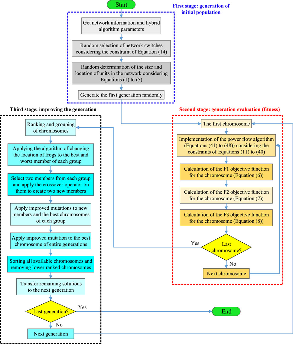
FIGURE 10. Structure flowchart of the proposed hybrid algorithm.
3.2.2 Step 1: generation of the initial population
At this stage of the model, an initial population will be created with a certain number of possible solutions that are randomly selected. In this step, there is a function that prevents the creation of duplicate solutions to have the maximum number of distinct solutions. Since in this problem, the goal is simultaneous placement and reconfiguration, according to Figure 11, each chromosome is composed of the state of several network switches, the size of units, and the location of units. The status of the switches is defined as open and closed by considering the constraint of Eq. 14, and the location and size of the units represent the power capacity of each unit that is installed in a specific bus and since each unit will a different capacity depending on the installation location, Eqs 1–5 should be considered in determining the location and size. Therefore, according to the probability of producing DG units in different time intervals, Eqs 1–5 are used.

FIGURE 11. Structure of each chromosome.
3.2.3 Step 2: generation evaluation (fitness)
In this step, voltage deviations, losses, and operating costs are calculated for all the produced solutions, and these values are used to calculate the fitness function of each chromosome. The values obtained for each solution provide the conditions for sorting the solutions as well as selecting the appropriate solutions in the next step. It should be noted that at this stage, the information obtained from the power flow algorithm is used to calculate the functions F1, F2, and F3.
3.2.4 Step 3: improving generation
In this stage of the model, according to the operators in the improved SFLA as well as the improved operators of GA, the new generation population is created. The improved mutation function, which has a substantial effect on raising the quality of solutions, is one of the most essential components of this stage. The mutation function in the normal genetic algorithm works in such a way that it randomly selects one or more genes from the chromosome and changes its value. However, by doing such work, the value of the fitness function of the chromosome may decrease and, thus, deviate from the optimal solution. Therefore, in the first part, it is necessary to prevent such a problem, the mutation function works in such a way that it does not reduce the value of the fitness function of the chromosome. For this purpose, in the improved mutation function, it is assumed that if the mutation causes a decrease in the value of the fitness function, changes on the chromosome should be omitted. Furthermore, because the selection of genes is carried out randomly and the change in the number of genes is made randomly, it is possible that in successive mutations during generations, due to the repetition of the selection of genes or the selection of inappropriate genes consecutively, the performance of the mutation function is greatly reduced and may not have a significant impact on the solutions. To increase the effect of the mutation function, the random selection of this function should undergo minor changes so that the nature of its randomness is not lost. For this purpose, each chromosome is assigned an array of suitable gene numbers for mutation. Furthermore, for each gene, an array of suitable options is assigned to select the value in the mutation function. The process of running the program is such that in each chromosome, the mutation function randomly selects the appropriate option from among the remaining available options, and if this gene change does not have a positive effect on the fitness function, it is selected from the arrays of appropriate options and the appropriate amount of each gene will be deleted. In this way, if there is no change in the best available chromosome in one generation, in the next generation, and when the mutation function is applied, the selection is still carried out randomly but in a more limited range. In this way, in addition to preventing a significant increase in calculation time, the accuracy and quality of optimal solutions will also increase. It should be noted that here, the mutation used in the improved SFLA is used instead of the mutation of GA.
4 Simulation results and discussion
The proposed method is implemented on the 33-bus distribution network in MATLAB software. The single-line diagram of the network is shown in Figure 12A, and the network includes 37 transmission lines of which lines 33–37 are open. To observe the effect of different devices on the network, the network load at peak time is 4.365 MW. The network load will change according to the pattern outlined by Soroudi et al. (2015) over 24 h, as shown in Figure 12B. Moreover, Figure 12C shows the network energy price in $/kW. In this research, it is assumed that two WT units with a capacity of 800 kW and two PV units with a capacity of 500 kW, whose output will be changed according to Hooshmand and Rabiee (2019), can be installed. Furthermore, an ESS unit with a capacity of 500 kWh, whose information is provided in the work of Carpinelli et al. (2013), can be installed in the network. In this study, similar to the work of Ghahramani et al. (2018), five types of EV units are used, and the type of vehicle is determined based on the driving pattern. In addition, one charging station for EVs is considered in the network. The maximum and minimum of each type of EV are 30 and 5, respectively. The total number of charging station EVs is 100. Information about EVs and the distance traveled by each type of EV in 24 h is provided in the work of Parvania et al. (2013). The factor δEV (v) in Eq. 37 is considered equal to 1/6 (kW/km). The cost that the distribution company pays in 24 h to buy electricity from the power injection units to the grid is determined according to the work of Parvania et al. (2013). Furthermore, the cost of lost energy VOLL is considered to be 1,000 $/MW in this research.
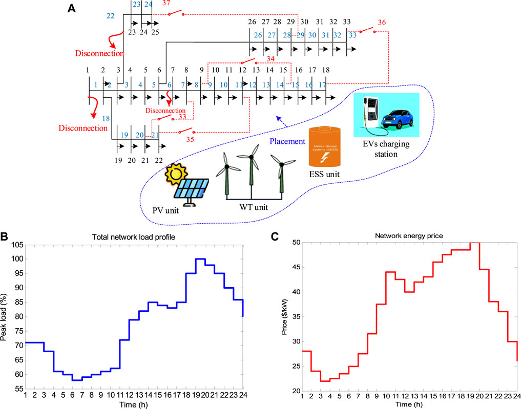
FIGURE 12. (A) Single-line diagram of the 33-bus distribution network, (B) total network load profile, and (C) network energy price (Soroudi et al., 2015).
In this section, to evaluate the proposed method, its performance is examined in four scenarios:
• Scenario 1: Reconfiguration and simultaneous placement in the network with the presence of all units (WT, PV, ESS, and charging station)
• Scenario 2: Simultaneous reconfiguration and placement in the network without considering ESSs and EVs
• Scenario 3: Placement in the network with all units and without considering reconfiguration
• Scenario 4: Network in a critical state
In this research, the goal is to optimize three objective functions F1, F2, and F3 using a hybrid GA-SFLA multi-objective algorithm based on obtaining the Pareto front of optimal solutions that have minimum voltage deviations, losses, and operating cost. In the following discussion, the results of its performance will be shown for different scenarios. In scenario 1, all units including WT, PV, EVs, and EV parking are present, and the network will have reconfiguration capability. In scenario 1, the cost of 24 h of operation is 3,094.75 $, the optimal location for installing WT is on buses 18 and 30, the optimal location for installing PV is on buses 10 and 16, and the optimal location for installing ESS and charging stations for EVs is on buses 16 and 32, respectively. Furthermore, the losses and voltage deviations during 24 h in scenario 1 are 729.84 kW and 3.624 p. u., respectively. In this scenario, lines with numbers 7, 9, 14, 15, and 24 are open. Figure 13 shows the level of power changes of network units along with the ESS charge level in scenario 1. It can be seen that the changes in charging and discharging states of the ESS can be defined according to the load pattern and energy price in such a way that the ESS is charged during off-peak load hours and discharged during peak load hours.
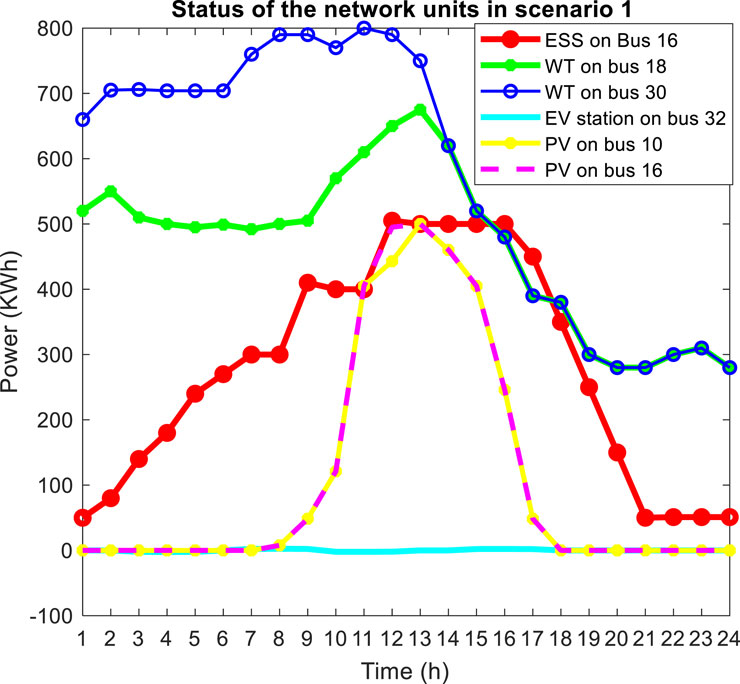
FIGURE 13. Level of power changes in network units in scenario 1.
Figure 14 shows the 3D Pareto front obtained from the final developed model for scenario 1. In this figure, the solutions of the first-generation hybrid GA–SFLA algorithm (orange dots) and the optimized solutions of the last generation (blue dots) are shown with different symbols. As shown in the figure, the minimum voltage deviations, losses, and operating costs in the first population are equal to 5.272 p. u., 745.73 kW, and 3,100.78 $, respectively. After running the program for 50 consecutive generations, the minimum voltage deviations, losses, and operating costs are equal to 3.624 p. u., 729.84 kW, and 3,094.75 $, respectively. These outputs indicate that the desired variables have been optimized during the progress of the generation. It can be pointed out that the population points of the last generation have improved significantly. In this way, the objective functions of F1, F2, and F3 of this generation have decreased compared to the first generation. In addition, the performance of the hybrid GA–SFLA algorithm is compared with the basic GA, which is shown in Figure 14 of the latest generation GA with a green symbol. In this algorithm, the best solutions are obtained as 9.041 p. u., 1803.36 kW, and 7,739.05 $ , which means that the hybrid GA–SFLA algorithm has a better performance of 2.5% than the basic GA in problem optimization. Finally, Figure 15 shows the average power flow from each network line during 24 h for scenario 1. For example, the power flow changes in lines 13, 17, and 18 are shown during 24 h, and it should be noted that the negative bars indicate the reverse direction of the power flow between the two buses.
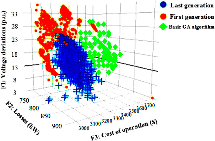
FIGURE 14. Pareto front obtained by the proposed hybrid algorithm.
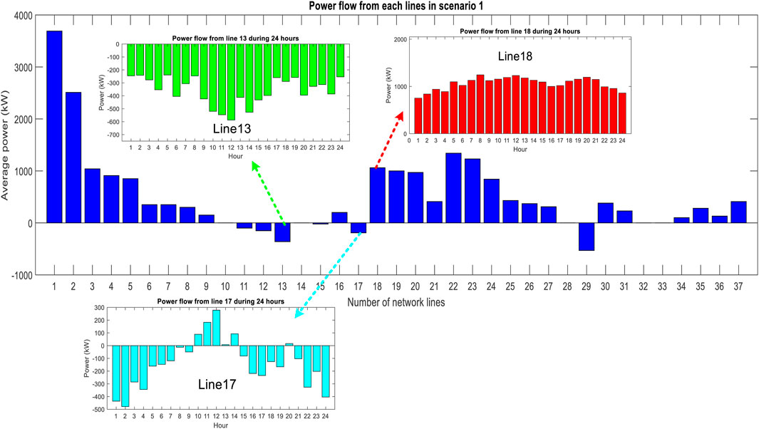
FIGURE 15. Power flow in network lines based on the average transmission value for scenario 1.
In scenario 2, there are no ESS and EV units, so the effect of the ESS and EVs on the network configuration, injected power from the upstream network, and DG power amount can be investigated. In this scenario, the 24-h operating cost of the network is 3,142.71 $, which has increased compared to scenario 1. The optimal installation location of WTs is on buses 18 and 30 and PVs on buses 15 and 31. Network losses and voltage deviations are equal to 1,263.33 kW and 8.783 p. u, respectively, which shows the effect of the ESS and EVs on reducing the three objective functions F1, F2, and F3. In scenario 2, lines with numbers 4, 7, 11, 13, and 16 are open.
Due to the low capacity of DG sources (500 kW) in both scenarios 1 and 2, with and without ESSs, DG sources generate their maximum possible power. Here, to observe the effect of the ESS and EVs on DG, it is assumed that the network with WTs with a capacity of 800 kW is investigated in two separate scenarios with and without ESSs and EVs. According to Figure 16, the presence of ESSs and EVs increases the generation capacity of DG resources. The comparison of the results of these two scenarios, where the capacity of WTs is 800 kW, is shown in Table 5.
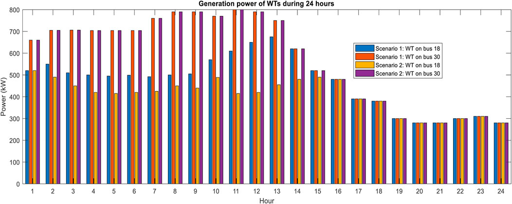
FIGURE 16. Generation power of WTs in scenarios 1 and 2.
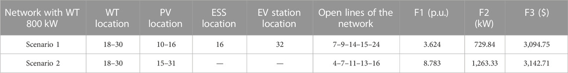
TABLE 5. Comparison of the results in two scenarios 1 and 2 with and without ESS and EVs with WT 800 kW.
In scenario 3, the network is evaluated in the initial configuration without considering the reconfiguration capability. The value of the F3 function in this scenario is 3,113.17 $. It can be said that network reconfiguration reduces the cost of operation, compared to scenario 2, it can be said that the effect of reconfiguration is less than that of the presence of ESSs and EVs. In this scenario, losses are equal to 1,105.12 kW and voltage deviations are equal to 7.211 p. u. In addition, in this scenario, WTs are installed on buses 14 and 32, PVs on buses 15 and 30, and EV charging stations and ESSs are installed on buses 14 and 32, respectively. The network is in its initial configuration, so lines with numbers 33 to 37 are open. As shown in Figure 17, the ESS and EV station charge level installed in this scenario is compared with scenario 1, which shows that the ESS and EV station charge level is affected by reconfiguration. Although both devices have the function of energy storage, ESSs can be used to support the network load and store the production power of the units, while the charging stations help to transport EVs and transfer energy to distant places. To better understand the issue, the performance of the ESS and EVs with different power levels is shown in Figure 17A. As shown in Figure 17B, due to the difference in the installation location of the EV station and the changes in the charge and discharge level of the station at different hours, the travel patterns in EVs have changed in scenarios 1 and 3, as shown in Figures 17C, D.
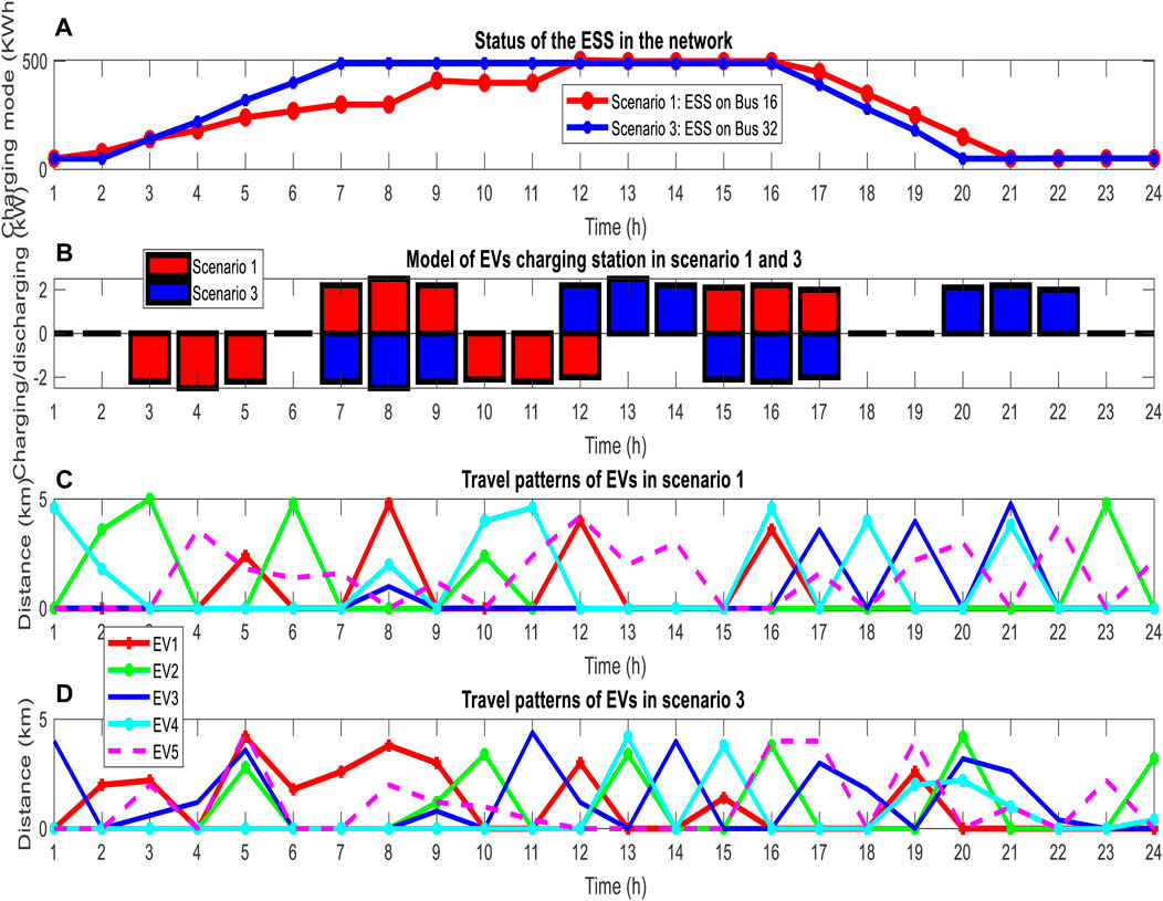
FIGURE 17. (A) ESS charge level changes in scenarios 1 and 3, (B) EV station charge level changes in scenarios 1 and 3, (C) travel patterns of EVs in scenario 1, and (D) travel patterns of EVs in scenario 3.
In scenario 4, according to Figure 12, it is assumed that the connection between the distribution network and the substation will be cut off between 8 and 10 o’clock, as well as lines 6 and 22. Here, to evaluate the effect of reconfiguration, the network is examined with and without considering the reconfiguration capability. In the case that the network has the capability of reconfiguration, the cost of operating the network in 24 h is 6,116.1 $, and in the case that the network does not have the capability of reconfiguration, this cost increases to 23,913.1 $, which is due to the number of lost loads in this case. As an example, bus 18 lost only 134 kW of load in the case with reconfiguration capability, while in the case without reconfiguration capability, the amount of load cut in this bus was 1,742 kW. Figure 18A shows the amount of load shedding in two modes with and without reconfiguration, and Figure 18B shows the cost difference between these two modes. As can be seen, with reconfiguration, we have been able to reduce the cost of load shedding in the entire network buses from 15,782 $ to 1,214 $, which has saved approximately 14,568 $. It can be said that reconfiguration will reduce the cost of the distribution company and also reduce the amount of interrupted load, which itself leads to the improvement of network resilience. In the case with reconfiguration capability, the optimal location to install WTs is on buses 30 and 32, PVs on buses 18 and 23, the ESS on bus 22, and the EV charging station on bus 3. Furthermore, lines numbered 9, 13, and 36 are assumed to be open and lines 6 and 22 are assumed to be disconnected. In the case without reconfiguration, the optimal location to install WTs is on buses 14 and 25, PVs on buses 7 and 11, the ESS on bus 6, and the EV charging station on bus 3. In addition, lines 6 and 22 are disconnected. In Figure 18C, the voltage profile in bus 18 is shown; as can be seen in the case without reconfiguration, the voltage of this bus is collapsing and exceeding the high voltage limit, which shows the effect of reconfiguration on network security from the point of view of voltage stability in critical times. Finally, to better compare the effect of network reconfiguration and the ESS on model outputs, the results of different scenarios are summarized in Table 6.
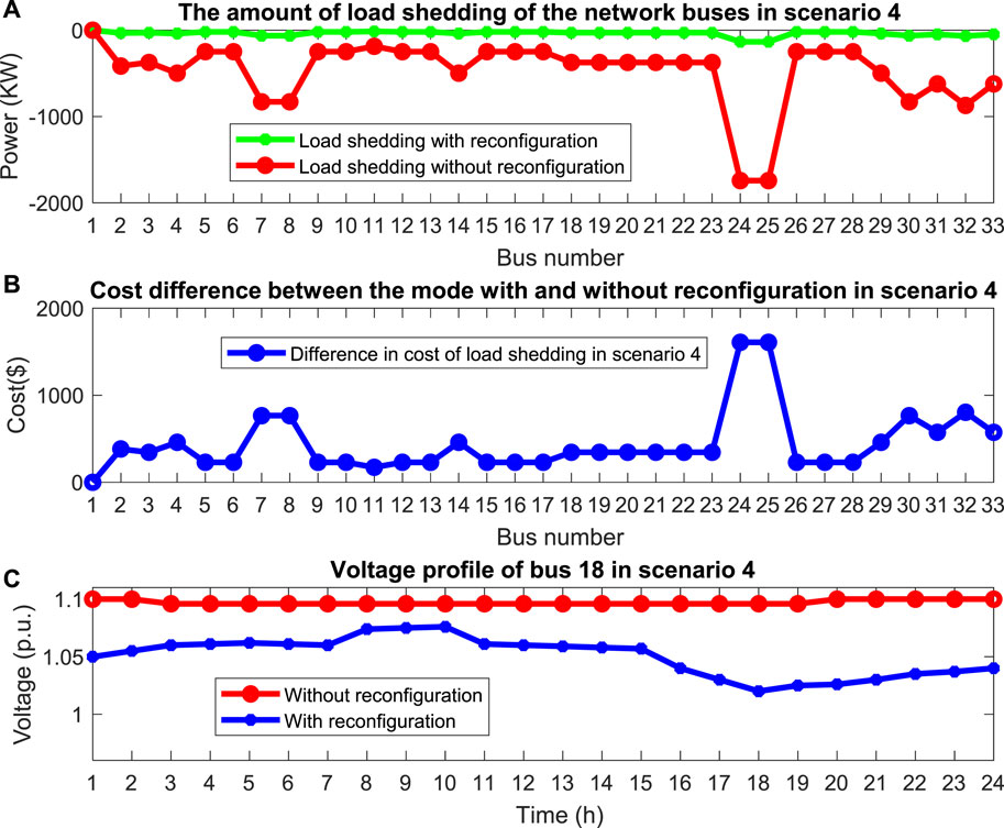
FIGURE 18. (A) Load shedding in scenario 4 with and without reconfiguration, (B) difference in the cost of load shedding between the two modes with and without reconfiguration, and (C) voltage profile in bus 18 in two cases with and without reconfiguration.
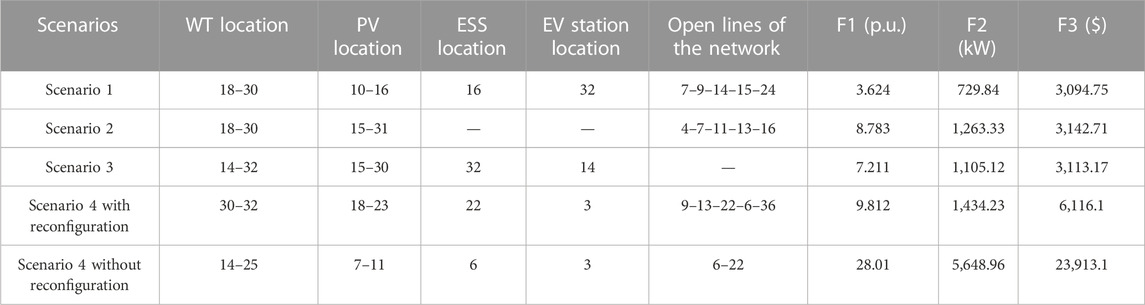
TABLE 6. Comparison of different scenarios of the network.
4.1 Performance evaluation of the hybrid GA–SFLA algorithm based on standard indicators
In this section, the performance of the hybrid GA–SFLA algorithm is compared with a non-dominated sorting genetic algorithm (NSGA-II) (Verma et al., 2021) based on standard indicators such as mean ideal distance (MID), maximum spread or diversity, spacing, and a number of Pareto solution (NPS), to evaluate the proposed algorithm. At first, these indicators are defined, and then, the results of the algorithms are presented. In general, unlike single-objective optimization, two main criteria including maintaining diversity among Pareto solutions and convergence to a set of Pareto solutions can be considered for multi-objective optimization. One of these criteria is maximum spread or diversity, which measures the length of the diameter of the space cube used by the end values of the objectives for the set of non-dominant solutions. Equation 51 shows the calculation procedure of this index. In our three-objective model, this criterion is equal to the Euclidean distance between three boundary solutions in the objective space. The bigger this criterion, the better the performance.
Using Eq. 52, the spacing criteria find the relative space of consecutive solutions. Here, the measured space is equal to the lowest value of the sum of the absolute values of the difference in the values of the objective functions between the ith solution and the solutions located in the final non-dominated group. It should be noted that this spacing criterion differs from the Euclidean minimum distance criterion between solutions.
Here, the NPS criterion presents the number of Pareto optimal solutions that can be found in each algorithm. In multi-objective discussions based on the Pareto approach, one of the objectives is to keep the fronts as close as possible to the origin of the coordinates; the MID criterion determines the distance of the fronts from the best value of the population. After defining the standard criteria, as shown in Figure 19, the performance of the proposed algorithm based on the four criteria is graphically compared with the NSGA-II. Then, based on the outputs, the algorithms have been studied and evaluated statistically with the help of variance analysis.
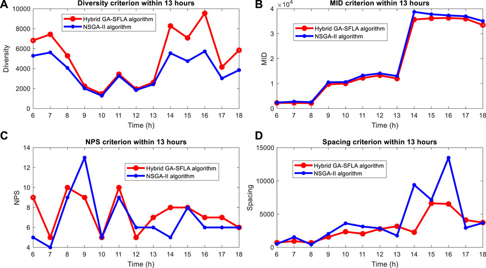
FIGURE 19. Comparison results of the proposed algorithms and NSGA-II based on (A) Diversity, (B) MID, (C) NPS and (D) Spacing criterion.
Figure 19 shows the performance results of the proposed algorithms and NSGA-II under the same conditions for scenario 1 within 13 h based on four defined standard criteria. As can be seen, the total value of MID, diversity, NPS, and spacing criteria in the proposed algorithm is better than NSGA-II. To evaluate and compare more accurately, we have used statistical analysis. As mentioned, in this section, we used variance analysis, the results of which are shown in Figure 20.
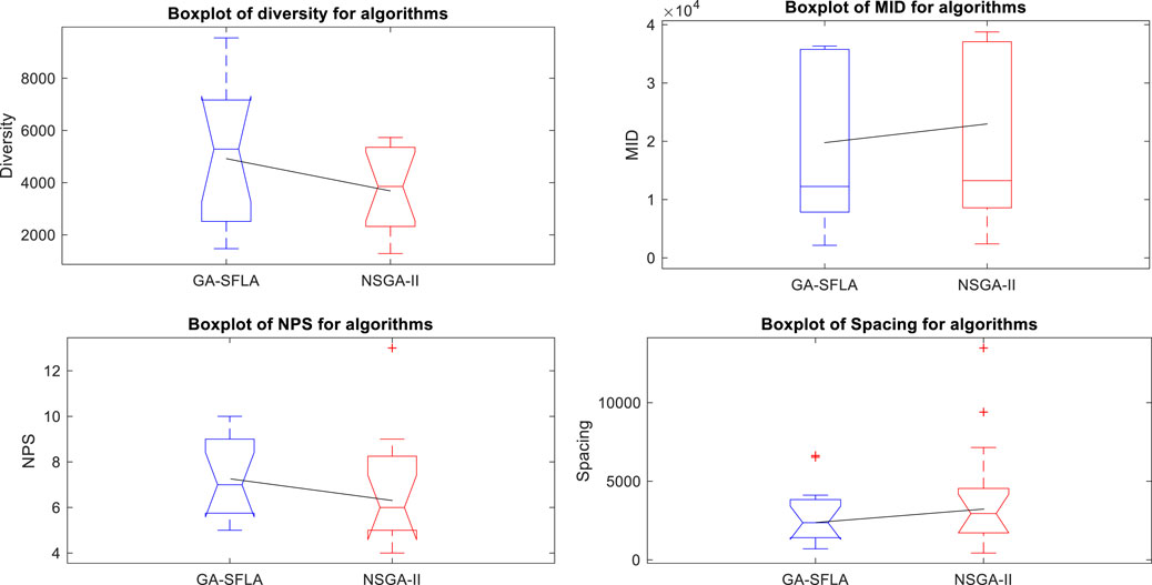
FIGURE 20. Box plot comparing the confidence interval based on the standard criteria of multi-objective algorithms.
Finally, a comparison was made between the proposed algorithm and other algorithms under the same conditions (assuming the same installation location of the units in the network) for scenario 1, and its results are shown in Table 7. As can be seen, the proposed algorithm has performed better in optimizing three objective functions.

TABLE 7. Comparison between the results of different algorithms for scenario 1.
5 Conclusion
In this article, various economic and technical objectives on the distribution network are investigated by presenting a multi-objective method and using the hybrid GA–SFLA algorithm. In this regard, three important tools are analyzed, which are reconfiguration, DG and ESS units, and EVs. The objective functions include voltage deviations, losses, and operating costs, the improvement of which leads to an increase in the technical quality of the system as well as an increase in the economic efficiency of the network. Here, a comprehensive model for distribution network reconfiguration based on the placement of ESS units, EVs, and DGs is presented, in which the effect of ESS units on the penetration of DGs and the network reconfiguration is evaluated. In addition, to show the effect of network reconfiguration on improving network resilience, the problem model is solved in a critical state. To solve the problem in different scenarios, an improved algorithm combining GA and ISFLA was used, and the results show that after increasing the number of generations, a significant improvement has occurred in the obtained solutions. Finally, a three-dimensional Pareto front is obtained to provide superior solutions, which indicates that the solutions improve significantly during the generations of algorithm execution. The simulation results show that simultaneous placement with reconfiguration with the proposed strategy has improved 1.98 times in the objective function of voltage deviations, reduced network losses by 375.28 kW, and reduced operating costs by 47.96$. Furthermore, under the same conditions, the proposed hybrid algorithm compared to the PSO, ISFLA, and ACO algorithms improved 6.496, 3.121, and 2.134 p. u., respectively, for objective function F1 and improved 1,471.59, 611.81, and 557.4 kW for objective function F2 and improved 4,758.37, 2,796.59, and 1772.7 $ for objective function F3. The evaluations of the proposed algorithm with other algorithms show its better performance, resulting in a 2.5% improvement compared to the basic GA. Finally, the obtained results can be expressed as follows:
• The distribution network configuration is affected by the presence of energy storage devices such as ESSs and EVs
• The optimal location of operation of DGs, ESSs, and EV charging stations is affected by network reconfiguration
• ESSs and EVs increase the penetration of DGs in the network
• Network reconfiguration is a suitable method to improve network resilience
• The reconfiguration of the distribution network can affect charging and discharging strategies
• Energy storage devices and network reconfiguration can reduce power losses individually or jointly
• The reconfiguration of the distribution network can improve the security of the network from the point of view of voltage stability in critical times
• Reconfiguration of the distribution network and energy storage devices plays a prominent role in reducing operating costs
• A hybrid GA–SFLA algorithm has a significant effect in optimizing three objective functions compared to similar algorithms such as GA and NSGA-II, resulting in performance improvement ranging between 1% and 2.5%
The findings of this study have several implications for future research in the field of distribution network optimization. The following areas can be explored:
1. Investigating the optimal integration of other renewable energy sources, such as solar and wind, into the distribution network along with DGs, ESS units, and EVs
2. Evaluating the impact of different load profiles and demand patterns on the optimal reconfiguration and placement of network components
3. Considering the uncertainties and variability associated with renewable energy sources and load demand in the optimization model
4. Exploring the potential benefits and challenges of implementing smart grid technologies and advanced control strategies in the distribution network
5. Assessing the environmental impacts and sustainability aspects of the proposed optimization strategies
Although this study has contributed significantly to the field, it is essential to acknowledge its limitations and challenges. Some potential areas of improvement and future research are as follows:
1. Enhancing the computational efficiency of the hybrid GA–SFLA algorithm to handle larger-scale distribution networks and more complex optimization problems
2. Incorporating more realistic and detailed models for the devices used in the network, such as considering the aging and degradation of DGs, ESS units, and EVs over time
3. Addressing the potential cybersecurity risks associated with the integration of advanced technologies and communication systems in the distribution network
In conclusion, the present study demonstrated the effectiveness of the hybrid GA–SFLA algorithm in optimizing multiple objective functions for distribution network reconfiguration and placement of DGs, ESS units, and EVs. The findings contribute to the existing body of knowledge and open up opportunities for future research in this field.
Data availability statement
The original contributions presented in the study are included in the article/Supplementary Material; further inquiries can be directed to the corresponding author.
Author contributions
YG: formal analysis, funding acquisition, visualization, methodology, and writing–review and editing. HK: conceptualization, supervision, and writing–original draft. KA: methodology, project administration, supervision, and writing–original draft. MA: investigation, software, visualization, and writing–review and editing. AY: formal analysis, funding acquisition, project administration, resources, validation, and writing–review and editing. MD: conceptualization, investigation, methodology, software, and writing–review and editing.
Funding
The authors declare financial support was received for the research, authorship, and/or publication of this article. The authors extend their appreciation to the Deanship of Scientific Research at Northern Border University, Arar, KSA, for funding this research work through the project number “NBU-FFR-2023-0140.” They also gratefully thank the Prince Faisal bin Khalid bin Sultan Research Chair in Renewable Energy Studies and Applications (PFCRE) at Northern Border University for their support and assistance.
Conflict of interest
The authors declare that the research was conducted in the absence of any commercial or financial relationships that could be construed as a potential conflict of interest.
Publisher’s note
All claims expressed in this article are solely those of the authors and do not necessarily represent those of their affiliated organizations, or those of the publisher, the editors, and the reviewers. Any product that may be evaluated in this article, or claim that may be made by its manufacturer, is not guaranteed or endorsed by the publisher.
References
Abul’Wafa, A. R. (2011). A new heuristic approach for optimal reconfiguration in distribution systems. Electr. Power Syst. Res. 81 (2), 282–289. doi:10.1016/j.epsr.2010.09.003
Ajmal, A. M., Ramachandaramurthy, V. K., Naderipour, A., and Ekanayake, J. B. (2021). Comparative analysis of two-step GA-based PV array reconfiguration technique and other reconfiguration techniques. Energy Convers. Manag. 230, 113806. doi:10.1016/j.enconman.2020.113806
Arandian, B., Rahmat-Allah, H., and Gholipour, E. (2014). Decreasing activity cost of a distribution system company by reconfiguration and power generation control of DGs based on shuffled frog leaping algorithm. Int. J. Electr. Power & Energy Syst. 61, 48–55. doi:10.1016/j.ijepes.2014.03.001
Arif, A., Wang, Z., Wang, J., and Chen, C. (2017). Power distribution system outage management with co-optimization of repairs, reconfiguration, and DG dispatch. IEEE Trans. Smart Grid 9 (5), 4109–4118. doi:10.1109/tsg.2017.2650917
Azizivahed, A., Narimani, H., Naderi, E., Fathi, M., and Narimani, M. R. (2017). A hybrid evolutionary algorithm for secure multi-objective distribution feeder reconfiguration. Energy 138, 355–373. doi:10.1016/j.energy.2017.07.102
Carpinelli, G., Celli, G., Mocci, S., Mottola, F., Pilo, F., and Proto, D. (2013). Optimal integration of distributed energy storage devices in smart grids. IEEE Trans. smart grid 4 (2), 985–995. doi:10.1109/tsg.2012.2231100
Dashtdar, M., Bajaj, M., and Hosseinimoghadam, S. M. S. (2022a). Design of optimal energy management system in a residential microgrid based on smart control. Smart Sci. 10 (1), 25–39. doi:10.1080/23080477.2021.1949882
Dashtdar, M., Bajaj, M., Hosseinimoghadam, S. M. S., Sami, I., Choudhury, S., Rehman, A. U., et al. (2021a). Improving voltage profile and reducing power losses based on reconfiguration and optimal placement of UPQC in the network by considering system reliability indices. Int. Trans. Electr. Energy Syst. 31 (11), e13120. doi:10.1002/2050-7038.13120
Dashtdar, M., Flah, A., Seyed Mohammad, S. H., Kotb, H., Jasińska, E., Gono, R., et al. (2022c). Optimal operation of microgrids with demand-side management based on a combination of genetic algorithm and artificial bee colony. Sustainability 14 (11), 6759. doi:10.3390/su14116759
Dashtdar, M., Najafi, M., and Esmaeilbeig, M. (2020). Calculating the locational marginal price and solving optimal power flow problem based on congestion management using GA-GSF algorithm. Electr. Eng. 102 (3), 1549–1566. doi:10.1007/s00202-020-00974-z
Dashtdar, M., Najafi, M., and Esmaeilbeig, M. (2021b). Reducing LMP and resolving the congestion of the lines based on placement and optimal size of DG in the power network using the GA-GSF algorithm. Electr. Eng. 103 (2), 1279–1306. doi:10.1007/s00202-020-01142-z
Dashtdar, M., Najafi, M., Esmaeilbeig, M., and Bajaj, M. (2022b). Placement and optimal size of DG in the distribution network based on nodal pricing reduction with nonlinear load model using the IABC algorithm. Sādhanā 47 (2), 73–17. doi:10.1007/s12046-022-01850-1
Ghahramani, M., Nojavan, S., Zare, K., and Mohammadi-ivatloo, B. (2018). “Short-term scheduling of future distribution network in high penetration of electric vehicles in deregulated energy market,” in Operation of distributed energy resources in smart distribution networks (Cambridge: Academic Press), 139–159.
Hamida, I. B., Brini Salah, S., Msahli, F., and Mohamed, F. M. (2018). Optimal network reconfiguration and renewable DG integration considering time sequence variation in load and DGs. Renew. energy 121, 66–80. doi:10.1016/j.renene.2017.12.106
Hassan, A. S., ElSaeed, A., Othman, F. M. B., and Ebrahim, M. A. (2022). Improving the techno-economic pattern for distributed generation-based distribution networks via nature-inspired optimization algorithms. Technol. Econ. Smart Grids Sustain. Energy 7 (1), 1–25. doi:10.1007/s40866-022-00128-z
Hooshmand, E., and Rabiee, A. (2019). Energy management in distribution systems, considering the impact of reconfiguration, RESs, ESSs, and DR: a trade-off between cost and reliability. Renew. energy 139, 346–358. doi:10.1016/j.renene.2019.02.101
Hosseinimoghadam, S. M. S., Dashtdar, M., Dashtdar, M., and Roghanian, H. (2020). Security control of islanded micro-grid based on adaptive neuro-fuzzy inference system. Sci. Bulletin” Ser. C Electr. Eng. Comput. Sci. 1, 189–204.
Jamian, J. J., Wardiah, M. D., Mokhlis, H., Mustafa, M. W., Lim, Zi J., and Abdullah, M. N. (2014). Power losses reduction via simultaneous optimal distributed generation output and reconfiguration using ABC optimization. J. Electr. Eng. Technol. 9 (4), 1229–1239. doi:10.5370/jeet.2014.9.4.1229
Jena, S., and Chauhan., S. (2016). “Solving distribution feeder reconfiguration and concurrent DG installation problems for power loss minimization by multi swarm cooperative PSO algorithm,” in Proceedings of the 2016 IEEE/PES Transmission and Distribution Conference and Exposition (T&D), Dallas, TX, USA, May 2016 (IEEE), 1–9.
Kahouli, O., Alsaif, H., Bouteraa, Y., Ali, N. B., and Mohamed, C. (2021). Power system reconfiguration in distribution network for improving reliability using genetic algorithm and particle swarm optimization. Appl. Sci. 11 (7), 3092. doi:10.3390/app11073092
Karthikeyan, N., Raj Pokhrel, B., Pillai, J. R., and Bak-Jensen., B. (2018). “Utilization of battery storage for flexible power management in active distribution networks,” in Proceedings of the 2018 IEEE Power & Energy Society General Meeting (PESGM), Portland, OR, USA, August 2018 (IEEE), 1–5.
Lotfi, H. (2020). Multi-objective energy management approach in distribution grid integrated with energy storage units considering the demand response program. Int. J. Energy Res. 44 (13), 10662–10681. doi:10.1002/er.5709
Lotfi, H. (2022). Multi-objective network reconfiguration and allocation of capacitor units in radial distribution system using an enhanced artificial bee colony optimization. Electr. Power Components Syst. 49 (13-14), 1130–1142. doi:10.1080/15325008.2022.2049661
Lotfi, H., and Ghazi, R. (2021). Optimal participation of demand response aggregators in reconfigurable distribution system considering photovoltaic and storage units. J. Ambient Intell. Humaniz. Comput. 12, 2233–2255. doi:10.1007/s12652-020-02322-2
Lotfi, H., Ghazi, R., and Naghibi-Sistani, M. B. (2020). Multi-objective dynamic distribution feeder reconfiguration along with capacitor allocation using a new hybrid evolutionary algorithm. Energy Syst. 11 (3), 779–809. doi:10.1007/s12667-019-00333-3
Mahboubi-Moghaddam, E., Mohammad, R. N., Khooban, M. H., Ali, A., and Javid sharifi, M. (2016). Multi-objective distribution feeder reconfiguration to improve transient stability, and minimize power loss and operation cost using an enhanced evolutionary algorithm at the presence of distributed generations. Int. J. Electr. Power & Energy Syst. 76, 35–43. doi:10.1016/j.ijepes.2015.09.007
Mahdavi, M., Haes Alhelou, H., Bagheri, A., Djokic, S. Z., and Ricardo Alan, V. R. (2021). A comprehensive review of metaheuristic methods for the reconfiguration of electric power distribution systems and comparison with a novel approach based on efficient genetic algorithm. IEEE Access 9, 122872–122906. doi:10.1109/access.2021.3109247
Mohammadi, M., Mohammadi Rozbahani, A., and Bahmanyar, S. (2017). Power loss reduction of distribution systems using BFO based optimal reconfiguration along with DG and shunt capacitor placement simultaneously in fuzzy framework. J. Central South Univ. 24 (1), 90–103. doi:10.1007/s11771-017-3412-1
Nasir, M. N. M., Shahrin, N. M., Bohari, Z. H., Sulaima, M. F., and Hassan, M. Y. (2014). “A Distribution Network Reconfiguration based on PSO: considering DGs sizing and allocation evaluation for voltage profile improvement,” in Proceedings of the 2014 IEEE Student Conference on Research and Development, Penang, Malaysia, December 2014 (IEEE), 1–6.
Nawaz, A., Wu, J., Ye, J., Dong, Y., and Long, C. (2023). Distributed MPC-based energy scheduling for islanded multi-microgrid considering battery degradation and cyclic life deterioration. Appl. Energy 329, 120168. doi:10.1016/j.apenergy.2022.120168
Nikkhah, S., and Rabiee, A. (2019). Multi-objective stochastic model for joint optimal allocation of DG units and network reconfiguration from DG owner’s and DisCo’s perspectives. Renew. energy 132, 471–485. doi:10.1016/j.renene.2018.08.032
Onlam, A., Yodphet, D., Chatthaworn, R., Surawanitkun, C., Siritaratiwat, A., and Khunkitti, P. (2019). Power loss minimization and voltage stability improvement in electrical distribution system via network reconfiguration and distributed generation placement using novel adaptive shuffled frogs leaping algorithm. Energies 12 (3), 553. doi:10.3390/en12030553
Parvania, M., Fotuhi-Firuzabad, M., and Shahidehpour, M. (2013). Optimal demand response aggregation in wholesale electricity markets. IEEE Trans. smart grid 4 (4), 1957–1965. doi:10.1109/tsg.2013.2257894
Quadri, I. A., and Bhowmick, S. (2020). A hybrid technique for simultaneous network reconfiguration and optimal placement of distributed generation resources. Soft Comput. 24 (15), 11315–11336. doi:10.1007/s00500-019-04597-w
Rafi, V., and Dhal, P. K. (2020a). “Loss minimization based distributed generator placement at radial distributed system using hybrid optimization technique,” in Proceedings of the 2020 International Conference on Computer Communication and Informatics (ICCCI), Coimbatore, India, January 2020 (IEEE), 1–6.
Rafi, V., and Dhal, P. K. (2020b). Maximization savings in distribution networks with optimal location of type-I distributed generator along with reconfiguration using PSO-DA optimization techniques. Mater. Today Proc. 33, 4094–4100. doi:10.1016/j.matpr.2020.06.547
Reddy, V., V.c., V. R., and T., G. M. (2018). Ant Lion optimization algorithm for optimal sizing of renewable energy resources for loss reduction in distribution systems. J. Electr. Syst. Inf. Technol. 5 (3), 663–680. doi:10.1016/j.jesit.2017.06.001
Saleh, O. A., Elshahed, M., and Elsayed, M. (2018). Enhancement of radial distribution network with distributed generation and system reconfiguration. J. Electr. Syst. 14 (3), 36–50.
Saonerkar, A. K., and Bagde, B. Y. (2014). “Optimized DG placement in radial distribution system with reconfiguration and capacitor placement using genetic algorithm,” in Proceedings of the 2014 IEEE international conference on advanced communications, control and computing technologies, Ramanathapuram, India, May 2014 (IEEE), 1077–1083.
Saonerkar, A. K., Tiwari, S., Pande, A. S., Sharma, P. G., and Bagde, B. Y. (2016). “Optimized distribution loss evaluation in ring main distribution system with DG placement, reconfiguration, and capacitor placement using GA,” in Proceedings of the 2016 International Conference on Inventive Computation Technologies (ICICT), Coimbatore, August 2016 (IEEE), 1–7.
Sedighizadeh, M., and Bakhtiary, R. (2016). Optimal multi-objective reconfiguration and capacitor placement of distribution systems with the Hybrid Big Bang–Big Crunch algorithm in the fuzzy framework. Ain Shams Eng. J. 7 (1), 113–129. doi:10.1016/j.asej.2015.11.018
Sedighizadeh, M., Esmaili, M., and Mahmoodi, M. M. (2017). Reconfiguration of distribution systems to improve reliability and reduce power losses using imperialist competitive algorithm. Iran. J. Electr. Electron. Eng. 13 (3), 287–302.
Sharma, S., Rehman Niazi, K., Verma, K., and Rawat, T. (2020). Impact of battery energy storage, controllable load, and network reconfiguration on contemporary distribution network under uncertain environment. IET Generation, Transm. Distribution 14 (21), 4719–4727. doi:10.1049/iet-gtd.2020.0369
Shi, Q., Li, F., Jin, D., Olama, M., Wang, X., Winstead, C., et al. (2022). Co-optimization of repairs and dynamic network reconfiguration for improved distribution system resilience. Appl. Energy 318, 119245. doi:10.1016/j.apenergy.2022.119245
Siahbalaee, J., Rezanejad, N., and Gevork, B. (2019). Gharehpetian. "Reconfiguration and DG sizing and placement using improved shuffled frog leaping algorithm. Electr. Power Components Syst. 47, 16–17. doi:10.1080/15325008.2019.1689449
Soroudi, A., Siano, P., and Keane, A. (2015). Optimal DR and ESS scheduling for distribution losses payments minimization under electricity price uncertainty. IEEE Trans. smart grid 7 (1), 261–272. doi:10.1109/tsg.2015.2453017
Sui, Q., Li, F., Wu, C., Feng, Z., Lin, X., Wei, F., et al. (2022). Optimal scheduling of battery charging–swapping systems for distribution network resilience enhancement. Energy Rep. 8, 6161–6170. doi:10.1016/j.egyr.2022.04.060
Teimourzadeh, H., and Mohammadi-Ivatloo, B. (2020). A three-dimensional group search optimization approach for simultaneous planning of distributed generation units and distribution network reconfiguration. Appl. Soft Comput. 88, 106012. doi:10.1016/j.asoc.2019.106012
Tolabi, H. B., Ali, M. H., and Rizwan, M. (2014). Simultaneous reconfiguration, optimal placement of DSTATCOM, and photovoltaic array in a distribution system based on fuzzy-ACO approach. IEEE Trans. Sustain. Energy 6 (1), 210–218. doi:10.1109/TSTE.2014.2364230
Truong Anh, V., Ngoc Ton, T., Thuan, T. N., and Duong, T. L. (2018). Two states for optimal position and capacity of distributed generators considering network reconfiguration for power loss minimization based on runner root algorithm. Energies 12, 106–111. doi:10.3390/en12010106
Verma, S., Pant, M., and Snasel, V. (2021). A comprehensive review on NSGA-II for multi-objective combinatorial optimization problems. Ieee Access 9, 57757–57791. doi:10.1109/access.2021.3070634
Zhang, X., Fu, Z., Chen, H., Mao, W., Liu, S., and Liu, G. (2019). Levy flight shuffle frog leaping algorithm based on differential perturbation and quasi-Newton search. IEEE Access 7, 116078–116093. doi:10.1109/access.2019.2936254
Glossary
Keywords: multi-objective functions, energy storage, distributed generation, electric vehicles, reconfiguration, placement, GA–SFLA algorithm
Citation: Ghadi YY, Kotb H, Aboras KM, Alqarni M, Yousef A, Dashtdar M and Alanazi A (2023) Reconfiguration and displacement of DG and EVs in distribution networks using a hybrid GA–SFLA multi-objective optimization algorithm. Front. Energy Res. 11:1304055. doi: 10.3389/fenrg.2023.1304055
Received: 28 September 2023; Accepted: 27 November 2023;
Published: 19 December 2023.
Edited by:
Deepak Kumar, Birla Institute of Technology, IndiaReviewed by:
Srinvasa Rao Gampa, Seshadri Rao Gudlavalleru Engineering College, IndiaHossein Lotfi, Hakim Sabzevari University, Iran
Copyright © 2023 Ghadi, Kotb, Aboras, Alqarni, Yousef, Dashtdar and Alanazi. This is an open-access article distributed under the terms of the Creative Commons Attribution License (CC BY). The use, distribution or reproduction in other forums is permitted, provided the original author(s) and the copyright owner(s) are credited and that the original publication in this journal is cited, in accordance with accepted academic practice. No use, distribution or reproduction is permitted which does not comply with these terms.
*Correspondence: Hossam Kotb, aG9zc2FtLmtvdGJAYWxleHUuZWR1LmVn