An ultra-short-term forecasting method for multivariate loads of user-level integrated energy systems in a microscopic perspective: based on multi-energy spatio-temporal coupling and dual-attention mechanism

An ultra-short-term multivariate load forecasting method under a microscopic perspective is proposed to address the characteristics of user-level integrated energy systems (UIES), which are small in scale and have large load fluctuations. Firstly, the spatio-temporal correlation of users’ energy use behavior within the UIES is analyzed, and a multivariate load input feature set in the form of a class image is constructed based on the various types of load units. Secondly, in order to maintain the feature independence and temporal integrity of each load during the feature extraction process, a deep neural network architecture with spatio-temporal coupling characteristics is designed. Among them, the multi-channel parallel convolutional neural network (MCNN) performs independent spatial feature extraction of the 2D load component pixel images at each moment in time, and feature fusion of various types of load features in high dimensional space. A bidirectional long short-term memory network (BiLSTM) is used as a feature sharing layer to perform temporal feature extraction on the fused load sequences. In addition, a spatial attention layer and a temporal attention layer are designed in this paper for the original input load pixel images and the fused load sequences, respectively, so that the model can better capture the important information. Finally, a multi-task learning approach based on the hard sharing mechanism achieves joint prediction of each load. The measured load data of a UIES is analyzed as an example to verify the superiority of the method proposed in this paper.

1 Introduction

Due to the swift economic and social growth, global warming, shortage of fossil energy and environmental pollution problems are becoming more and more prominent (Ji et al., 2018). Promoting the transformation of the traditional energy system, to improve the efficiency of energy utilisation and to reduce carbon emissions is currently a major issue facing the global energy industry (Cheng et al., 2019a). The traditional energy system is limited to the independent planning, design and operation of energy systems such as electricity, gas, heat and cold, which artificially severs the coupling relationship between different types of energy sources, and is unable to give full play to the complementary advantages between energy sources (Wang et al., 2019). Energy utilisation efficiency, renewable energy consumption, energy conservation and emission reduction have all encountered bottlenecks (Cheng et al, 2019b). In response to the above problems, the concepts of energy internet (EI) and integrated energy system (IES) have been put forward and highly valued by many countries, which emphasise the development mode of changing from the production and supply of each energy source to the operation of joint scheduling of multiple energy sources (Li et al., 2018; Li and Xu, 2018; Zhu et al., 2021). Among them, IES, as an important physical carrier of EI, is an important energy utilisation method in the process of energy transition, as well as an effective method to promote renewable energy consumption and improve energy efficiency (Wu et al., 2016). User-side multivariate load ultra-short-term prediction as the IES optimal scheduling, the primary premise of energy management, is no longer limited to the independent prediction of a single energy consumption, it must take into account multiple energy systems at the same time (Li et al., 2022), which puts forward higher requirements for the accuracy and reliability of the IES multivariate load prediction, and it has become one of the research hotspots in the energy field at the present time.

Theoretically, traditional load forecasting has developed into a more developed system that focuses mostly on single loads like electricity, natural gas, cooling, and heating. Data-driven artificial intelligence techniques have been extensively employed in the research of load forecasting applications since the emergence of a new generation of artificial intelligence technology. On a technological level, there are two general groups of AI-based load prediction techniques: deep learning techniques and conventional machine learning techniques.

To accurately anticipate daily peak demand for the next month, Gao et al. (2022a) used a hybrid of extreme gradient boosting (XGBoost) and multiple linear regression (MLR). Short-term load forecasting in the literature (Singh et al., 2017) was accomplished with the help of a three-layer feedforward artificial neural network (ANN). For predicting the following day’s electrical usage over a period of 24 h, a support vector regression machine (SVM) based technique was presented in the literature (Sousa et al., 2014). Short-term electric demand forecasting using a hybrid model based on feature filtering convolutional neural network (CNN) with long and short-term memory was developed by Lu et al. (2019). Short-term cold load prediction in buildings using deep learning algorithms was achieved by Fan et al. (2017). It was suggested by Gao et al. (2022b) to forecast the cold load of big commercial buildings using a hybrid prediction model based on random forest (RF) and extreme learning machine (ELM), and the benefits of this model were validated in terms of time complexity and its own superior generalisation ability. Xue et al. (2019) proposed a heat load prediction framework based on multiple machine learning algorithms, such as SVM, deep neural network (DNN), and XGBoost, and then implemented a multi-step ahead heating load prediction in a district heating system to verify the superiority of the recursive strategy. A novel empirical wavelet transform (EWT) technique has been developed in the literature (Al-Musaylh et al., 2021) for revealing the intrinsic patterns in daily natural gas consumption demand data. For short-term gas load forecasting, Xu and Zhu, 2021 created a neural network that combines a time-domain convolutional network (TCN) with a bi-directional gated recurrent unit (BiGRU).

The foundation of conventional machine learning techniques is feature engineering, which is labor-intensive, sensitive to noise and outliers, and inefficient when dealing with high-dimensional data. Contrarily, the multi-layer mapping of deep learning allows for the effective extraction of the data’s deep characteristics, greatly enhancing the model’s capacity to represent the pattern of sample distribution. As a result, it demonstrates improved load forecasting prediction accuracy.

In fact, traditional energy system studies focus on a single type of energy, while IES considers diverse energy demands and focuses on high-quality multi-class energy studies (Hu et al., 2019). If the traditional single-load prediction method is still used, it is difficult to capture the correlation characteristics between different loads, and the prediction accuracy cannot be guaranteed. Therefore, how to properly dispose of the coupling relationship between multiple loads, set a more complete input feature set, effectively learn multiple energy coupling information, and achieve accurate IES multiple load forecasting based on this information is the focus of current research. The main mainstream techniques to deal with the coupling are multivariate phase space reconstruction (MPSR) (Zhao et al., 2016), multi-task learning (MTL) (Shi et al., 2018), and convolutional neural networks (CNN) (Li et al., 2022). In addition, Bai et al. (2022) utilized the minimum redundancy maximum relevance (MRMR) to screen feature sequences and the Seq2Seq model based on the dual attention mechanism to learn the spatio-temporal properties of urban energy load sequences. The above literature verifies that considering the coupling characteristics among loads helps to improve the forecasting accuracy, and also verifies the role of the attention mechanism.

Previously, IES load prediction models have focused on single-load independent prediction, while single-task load prediction methods consider every prediction task simply, mutually independent subproblem, which ignores the coupling relationships within multiple source loads in IES (Zhu et al., 2019). Multi-task learning improves model generalization by using a shared mechanism to train multiple tasks in parallel to obtain information implicit in multiple related tasks. In recent years, multi-task learning has been gradually applied to IES multivariate load prediction. Niu et al. (2022) constructed a new multi-task loss function weight optimisation method to search for optimal multi-task weights for balanced multi-task learning (MTL), which improves the prediction of IES multivariate loads.

Currently, the vast majority of studies on IES multivariate load forecasting are limited to macroscopic class load forecasting methods, focusing only on mining the correlation between each load’s own sequence and sequences of other external macro-factors. However, in some cases, the load variation patterns of different load nodes (e.g., substations, parks, and customers) within the same region may be potentially correlated in space and time due to the same external factors (e.g., weather and electricity prices). In order to improve the IES multiple load forecasting method, it is necessary to consider the spatial and temporal correlation of each load node in the IES. At this stage, the research on IES multiple load forecasting based on microscopic class load forecasting methods is still in its infancy. Compared with the previous studies, the contributions of this paper are as follows.

(1) The spatio-temporal correlation of the energy-using behavior of each load unit in the UIES is comprehensively analyzed, and each load unit is defined as a load pixel point. Based on the strong correlation of adjacent pixel points in static images and with reference to the storage method of color images, an IES multivariate load input feature set in the form of image-like based on the microscopic class load prediction method is proposed, which is a novel method for constructing the IES input feature set.

(2) A deep spatio-temporal feature extraction network (MCNN-BiLSTM) for multivariate load prediction is proposed. Among them, MCNN is used to perform independent spatial feature extraction for each load component pixel image, and BiLSTM is used to realize temporal feature extraction for fused load features at each time step. To realize end-to-end training from space to time and collaborative mining of spatio-temporal information.

(3) A multi-head attention mechanism is introduced in the spatial and temporal dimensions, respectively. This attention mechanism is a plug-and-play module that is placed before MCNN and before BiLSTM to enable the model to pay differential attention to the information in the original input load pixel image and the fused load sequence during the learning process.

(4) Using BiLSTM as the feature sharing layer, a multi-task learning approach under the hard sharing mechanism is adopted to further learn the inherent coupling information among electricity, heat, and cold loads. In order to adapt to the characteristics of the fluctuation of the three load profiles, as well as to explore the correlation of each load with meteorological factors and calendar rules, three fully connected neural networks with different structures are designed as feature interpretation modules.

2 User-level IES load characterization

2.1 User-level IES energy coupling mechanism

A user-level IES is an integrated energy system constructed at the distribution and usage levels to meet the diversified energy needs of multiple types of users, such as industrial parks, commercial centres, residential buildings and educational institutions. A typical interactive structure of a user-level IES is shown in Figure 1, which can be roughly divided into the IES side and the end-user side. On the IES side, the IES service provider conducts accurate multiple load forecasting based on the metered data of users’ energy consumption of electricity, heat, cooling, etc. collected in real time through intelligent terminals, so as to coordinate the transformation, storage, and distribution of energy sources within the IES to satisfy the diversified energy demand of users.

FIGURE 1

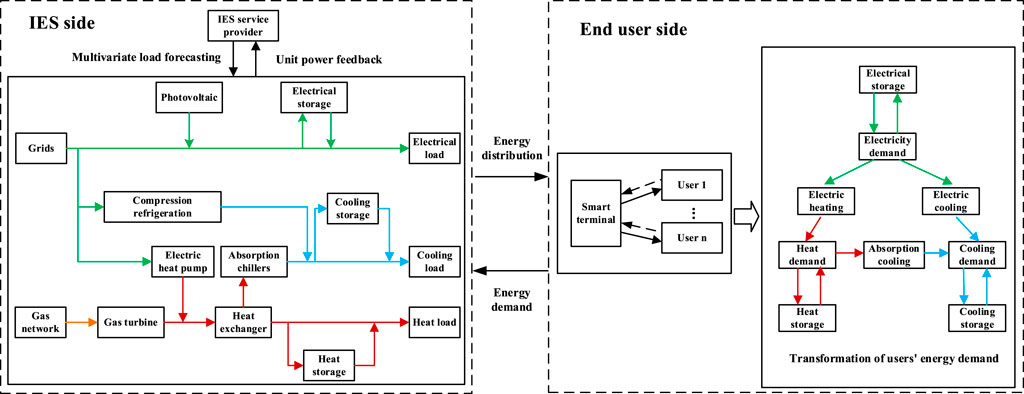
FIGURE 1. Simplified model of the UIES interaction structure.

In IES operation, external energy inputs come from the grid and the natural gas network, internal energy generation comes from rooftop photovoltaic systems and micro-gas turbines, various energy conversion equipment couples the different energy systems in a flow of energy, and energy storage equipment is used to increase the economy and flexibility of the system operation. The IES provider’s ability to provide electricity, heat, and cooling to its customers for a variety of energy needs is significantly affected by meteorological conditions, day-type information and building characteristics. In terms of meteorological conditions, the demand for heating and cooling loads varies seasonally with the gradual change in temperature. In terms of day-type information, the difference in human production activities between weekdays and holidays results in differences in energy demand. In terms of building characteristics, different system functions are important reasons for influencing the characteristics of energy use. Industrial areas tend to consume large amounts of electrical loads, and the cooling and heating loads play an auxiliary role to jointly serve the production schedule. The fluctuation of cooling and heating loads in commercial and living areas is closely related to human activities and shows some correlation. Figure 2 shows the variation of the total electric, thermal and cooling loads of the user-level IES studied in this paper under four seasons of the year, and the temperature variation under the corresponding moments.

FIGURE 2

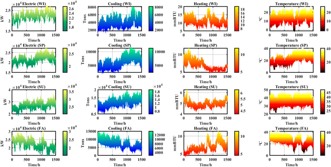
FIGURE 2. Multi-energy load correlation analysis of UIES.

As can be seen from Figure 2, the fluctuation of various types of loads in this UIES is accompanied by obvious seasonal changes. And the degree of coupling between the loads under different time periods has a certain degree of variability. Among them, the demand size of each load in summer and winter seasons has a large difference, which is especially obvious in the hot and cold loads. The spring and autumn seasons show a clear transition, with the change of temperature, the fluctuation of the hot and cold loads show a diametrically opposite trend, and the cold loads show a high degree of consistency between the overall external morphology and the temperature change. In addition, the overall trend of electric load and cold load is consistent in different periods, which indicates that the change in demand for cold load also affects the level of electric energy consumption.

2.2 Spatial correlation analysis of load units

In this paper, buildings and activity places with load collection equipment are defined as load units in the UIES, and the macro load sequence of the UIES is aggregated from the corresponding micro load sequence of each load unit. In UIES, the energy consumption behavior of users is a dual reflection of the energy demand of load units at both macro and micro levels, which depends on macro-level factors such as energy price fluctuations, climate seasons, day-type information, etc., as well as micro-level factors such as regional planning layout and building design characteristics. At the macro level, UIES is confined to smaller spatial scales, load units are influenced by the same microclimatic conditions in the same local area, and the energy use behavior of users maintains a certain degree of consistency. At the micro level, load units with similar geospatial locations or with the same functional attributes tend to have similar energy use habits. However, the types of load units with different functional attributes and their building sizes are often different, which directly leads to some differences in users’ energy use habits, energy end-uses (cooling, heating, lighting, etc.) and the proportion of each energy consumption. In addition, users’ energy use behavior can be simultaneously affected by equipment accidents and maintenance, extreme weather, major events and other emergencies, resulting in sudden changes in loads. Figure 3 shows the electrical, thermal and cooling load change curves for the nine load units in the UIES over a 240-h period.

FIGURE 3

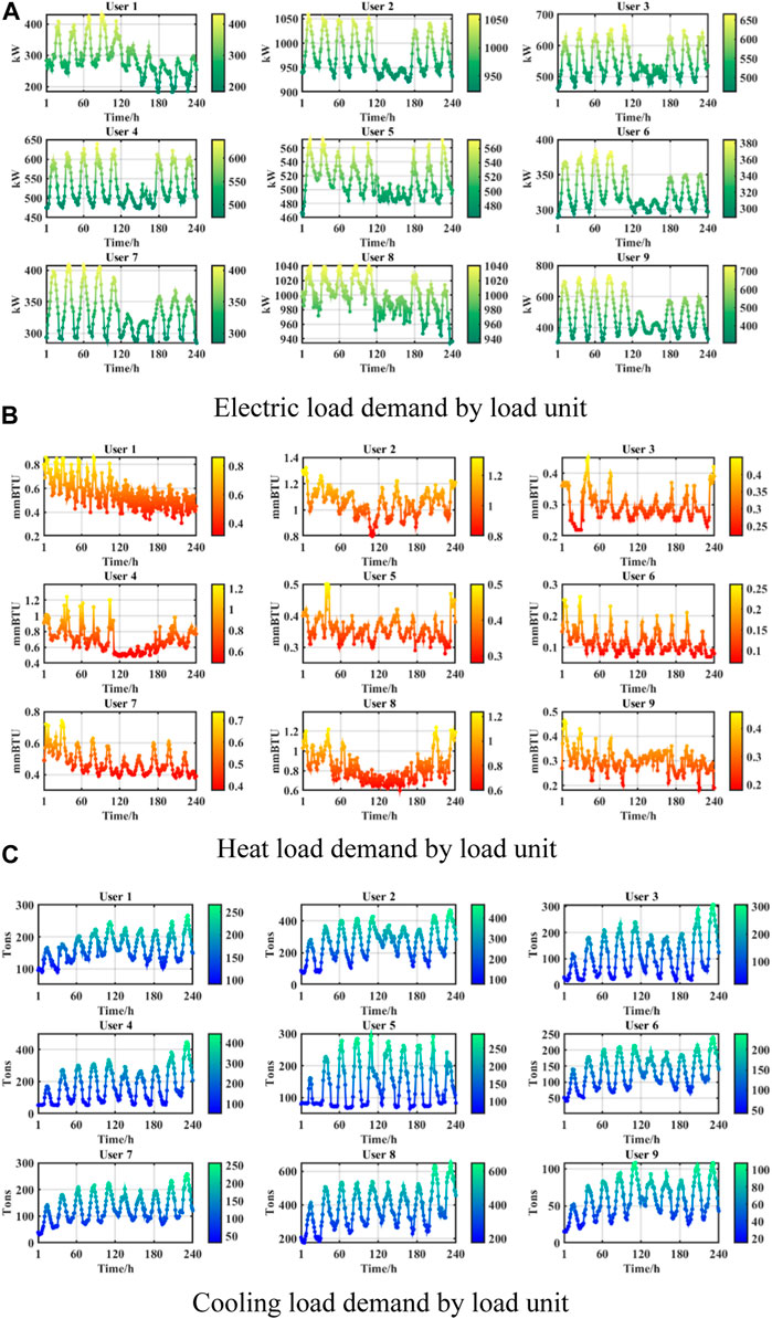
FIGURE 3. Demand for various types of energy of load units. (A) Electric load demand by load unit. (B) Heat load demand by load unit. (C) Cooling 199 load demand by load unit.

As can be seen in Figure 3, the three types of loads in each load unit exhibit a high degree of variability in their external patterns. Among them, the electrical load is significantly affected by the variation of day types. In addition to User1, the load change patterns of User2 to User9 have some correlation, which is manifested as having continuous fixed large peaks on weekdays and certain small peaks on double holidays. The fluctuation of the cold load has no obvious weekday or double holiday pattern, showing a gradual increase in progressive change. For the heat load, affected by the climate characteristics, its demand scale is much smaller than the electricity, cold load, the user heat behavior is more random. In addition to User3, User6 and User7 heat load changes have a certain correlation, the rest of the heat load fluctuation of the load unit has a strong randomness and time-varying changes, the cyclical law of change is not traceable.

After the above analysis, it can be seen that the non-independence of load change of load unit is not only related to its own building functional characteristics, scale size, location and other factors, but also has a close connection with local climate characteristics and calendar rules. Various types of load units are complex aggregates with broad spatial correlation. Therefore, the load change of each load unit is the deeper “implied information” in the change rule of the total load of UIES, and it is the “underlying logic” that reveals the characteristics of the total load’s external form, which contains a wealth of information to be mined.

2.3 Temporal correlation analysis of load units

Time correlation analysis is an essential and important part of load forecasting work. Referring to time correlation can select reasonable historical load variation intervals as input features in the subsequent actual load forecasting work, which is helpful to improve the model learning efficiency and reduce the computational overhead of the model. Therefore, in this paper, a certain number of load units are randomly selected for time correlation analysis based on Pearson correlation coefficients, which are shown in Figure 4.

FIGURE 4

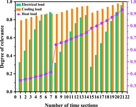
FIGURE 4. Time correlation analysis.

In Figure 4, the time sections of historical data selected in this paper are the first seven historical moments (numbered 15–21) from the current moment $\left(t+1\right)$, the $t+1$ moment and the first six moments a day ago (numbered 8–14), and the $t+1$ moment and the first six moments a week ago (numbered 1–7). According to the results of the time correlation analysis, the fluctuation of electric and cold loads has an obvious cyclical law of change, and the load at the current moment is not only affected by the load at the neighbouring historical moment but also has a strong correlation with the load at the same moment a day and a week ago. Among them, the fluctuation change of the cold load is the most stable and has strong predictability. While the temporal correlation of heat load gradually decreases with the increase in time interval, This is because changes in heat load demand are easily influenced by external factors. When the time span is large, the external factors change a lot, resulting in the heat load fluctuation no longer having a clear regularity.

3 Integrated load pixel image construction and spatio-temporal feature extraction

3.1 Integrated load pixel image construction

Compared with the inter-regional level IES and regional level IES, the UIES is smaller in size, its lack of random error elimination due to load aggregation effect, and greater load volatility. It is sometimes difficult to generalize the internal change pattern of each total load in the UIES if the macroscopic class load forecasting method is adopted. From the analysis in Subsections 2.2 and 2.3, it can be seen that the load data of each load unit in the UIES contains a large amount of spatio-temporal data, which is the most intuitive characteristic information for portraying the change patterns of each type of total load in the UIES.

This paper is based on a microscopic class load forecasting method, which focuses on the energy demand of each load unit in the UIES region, and ultimately produces the overall consumption forecast results for each type of energy in the UIES. Compared with the macroscopic class load forecasting method, this type of method explores the energy consumption characteristics of users from within the region, and its modeling is more detailed and thorough, so that more accurate forecast results can be obtained.

Usually, there is a strong correlation between a pixel point of a static image and its relative neighbouring pixel points, so in the field of image recognition, convolutional neural networks are often able to capture the local features of an image through a small receptive field so as to form a feature quantity with certain regularity and correlation in the high-dimensional space. Based on the analysis in subsection 2.2, it can be seen that there is also a certain correlation between the load units of UIES, and the correlation is more significant for load units with the same functional attributes and closer geospatial locations, which is similar to the pixel law of still images. Analogous to the application of CNN in the field of image recognition, as shown in Figure 5. In this paper, each load unit in the studied UIES is regarded as a load pixel point, and the local feature extraction capability of CNN is used to mine the hidden information among load units from local to global perspectives so as to realize ultra-short-term prediction of various types of total loads in the UIES.

FIGURE 5

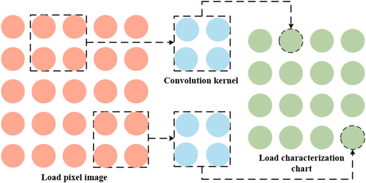
FIGURE 5. CNN-based feature extraction for load pixel images.

For a colour image, each pixel contains the three colour components of RGB, which can be regarded as a superposition of three layers of two-dimensional arrays, each layer representing a color channel. In the context of this paper, each load unit in UIES has different levels of demand for electricity, heat and cold, so load unit contains the characteristic information of three kinds of loads. Following the storage form of color images, each load pixel follows a certain arrangement to form a comprehensive load pixel image, which consists of three load component images of electricity, heat and cold. In this paper, from the functional characteristics of the load units contained in the studied UIES, the load units are divided into several categories according to their functional attributes, and the load units with close spatial locations in each category are arranged closely. For example, the UIES under study contains $N$ load units, which constitute a composite load pixel image of length and width $\lceil \sqrt{N}\rceil$. The load units of each attribute category are filled with load pixel points of each row along the image column direction in turn, and finally the blank load pixel points are processed by complementary 0.

Based on the analyses in subsection 2.3, the integrated load pixel images with different time delays from the predicted moment are constructed separately, as shown in Figure 6. In this paper, the integrated load pixel image at each moment is regarded as a frame of $\left(\lceil \sqrt{N}\rceil \times \lceil \sqrt{N}\rceil \right)$, and the load demand fluctuation of each load unit in the time period $\left(t-h+1,t\right)$ can be reflected by stacking $h$ frames. In this way, the input feature is a three-dimensional matrix with spatio-temporal information and covering the three load coupling features at the same time, while the output feature is the total electric, thermal and cooling loads at the moment $t+1$ to be predicted.

FIGURE 6

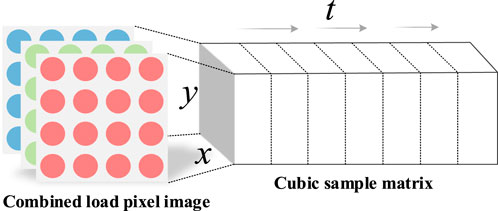
FIGURE 6. Integrated load pixel images at different moments.

3.2 Spatial feature extraction based on parallel multichannel convolutional neural network

When CNN performs feature extraction on colour images, it uses the multi-channel mechanism to access the three colour channels of the colour image. Although the load pixel image constructed in this paper has similarities with the colour image, the three load components of the load pixel are more independent and have different meanings compared to the RGB components of the pixel points. Therefore, two aspects should be taken into account when using CNN for the spatial feature extraction of load pixels. One is that the feature independence of each load itself should be preserved in the feature extraction process. Second, the input features in this paper are loading pixel images at different moments, which need to be formed into a standard time-step format before subsequent time-dependent capturing. If the multi-channel mechanism of CNN is directly used to extract features from the load pixel images at different moments, the feature information of the three loads at different moments will be fused at the same time in the first convolution process, and the independence and temporal integrity of the loads embedded in the input sequences will not be preserved. Therefore, in this paper, a multi-channel parallel CNN structure is designed for the research context. Figure 7 shows its network architecture.

FIGURE 7

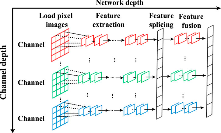
FIGURE 7. Multi-channel feature extraction CNN network structure.

In Figure 7, the multichannel convolutional neural network (MCNN) constructed in this paper has the dual characteristics of channel depth and network depth. In the channel depth direction, no information is exchanged between each feature extraction channel until feature fusion, and the own features of each load component image under each time section are extracted separately and independently. The spatial characteristics of the load pixels are extracted in a sub-category, time-segmented manner. Therefore, the number of channels of MCNN is always kept as $T_{se}\times N_{lo}$ during feature extraction, where $T_{se}$ is the number of time sections and $N_{lo}$ is the number of load types in the studied IES. In the direction of network depth, considering that increasing the pooling layer will accelerate the convergence speed of the network but also cause certain information loss phenomenon, so this paper only uses the convolutional layer for feature extraction. For a certain channel, the feature extraction process is shown below.

${\mathit{C}}_{i,j}^{\left(k\right)}=f\left({\displaystyle \sum _{S=1}^M}{\mathit{C}}_{S,j-1}^{\left(k\right)}\otimes {\mathit{W}}_{i,j}^{\left(k\right)}+{\mathit{b}}_{i,j}^{\left(k\right)}\right){\mathit{C}}_{\mathrm{0,0}}^{\left(k\right)}\in \mathit{G}(1)$

In the formula: ${\mathit{C}}_{S,j-1}^{\left(k\right)}$ is the $S$-th feature map in the $j-1$-th convolution layer of the $k$-th channel; ${\mathit{W}}_{i,j}^{\left(k\right)}$ is the weight matrix of the $i$-th convolution kernel in the $j$-th convolution layer of the $k$-th channel; ${\mathit{b}}_{i,j}^{\left(k\right)}$ is the bias matrix; ${\mathit{C}}_{i,j}^{\left(k\right)}$ is a feature map output from the $j$-th convolution layer; $\otimes$ is the convolution operation; $f$ is the activation function; $M$ is the number of feature maps; $\mathit{G}$ is the original set of each load pixel image; ${\mathit{C}}_{\mathrm{0,0}}^{\left(k\right)}$ is a load component image under a certain time section of the input to the $k$-th channel.

On the basis of MCNN fully extracting each load component image under each time section, the final number of feature maps output by all channels is $T_{se}\times N_{lo}\times M_{nu}$, where $M_{nu}$ is the number of convolution kernels in the last convolution layer of each channel. It can be seen that the spatial features of each type of load output by MCNN not only maintain the feature independence of each load itself, but also retain the information of the time dimension of each load feature, which can be expressed as:

${\mathit{C}}^{e,h,c}=\left[{\mathit{C}}_{t-h+1}^e,{\mathit{C}}_{t-h+1}^h,{\mathit{C}}_{t-h+1}^c,\cdots ,{\mathit{C}}_t^e,{\mathit{C}}_t^h,{\mathit{C}}_t^c\right](2)$

In the formula: ${\mathit{C}}^{e,h,c}$ is the set of feature maps for the output of each channel of the MCNN; ${\mathit{C}}^e$, ${\mathit{C}}^h$, ${\mathit{C}}^c$ are the set of spatial characteristic maps of electrical, thermal and cooling loads at a given moment in time, respectively.

Before proceeding with the subsequent temporal feature extraction, the spatial features of various types of loads at the same moment in time need to be fused again using the multi-channel mechanism. At this time, the number of channels of MCNN is $T_{se}$, and the input features of each channel are under the same moment ${\mathit{C}}^e$, ${\mathit{C}}^h$, ${\mathit{C}}^c$. Finally, the output fused load feature maps of each channel are flattened and the features are spliced in chronological order in order to form a fused load feature sequence with a standard time step, as shown in the following equation:

$\mathit{R}=\left[{\mathit{F}}_{t-h+1},{\mathit{F}}_{t-h+2},\cdots ,{\mathit{F}}_t\right](3)$

In the formula: $\mathit{R}$ is the fused load feature sequence; $\mathit{F}$ is the fused load feature vector at a certain time section.

3.3 Time-dependent capture based on bidirectional long and short-term memory networks

LSTM is a variant of the traditional recurrent neural network (RNN), which is improved by introducing input gates, forgetting gates, and output gates, thus solving the long-term dependence problem of RNN in the training process and avoiding the gradient explosion and gradient dispersion phenomenon. The rules for calculating each variable in LSTM are shown below.

$\left\{\begin{array}{l}{\mathit{u}}_t=\mathit{\sigma }\left({\mathit{W}}_{xu}{\mathit{x}}_t+{\mathit{W}}_{hu}{\mathit{h}}_{t-1}+{\mathit{b}}_u\right)\\ {\mathit{f}}_t=\mathit{\sigma }\left({\mathit{W}}_{xf}{\mathit{x}}_t+{\mathit{W}}_{hf}{\mathit{h}}_{t-1}+{\mathit{b}}_f\right)\\ {\mathit{o}}_t=\mathit{\sigma }\left({\mathit{W}}_{xo}{\mathit{x}}_t+{\mathit{W}}_{ho}{\mathit{h}}_{t-1}+{\mathit{b}}_o\right)\\ {\mathit{g}}_t=\mathit{tanh}\left({\mathit{W}}_{xg}{\mathit{x}}_t+{\mathit{W}}_{hg}{\mathit{h}}_{t-1}+{\mathit{b}}_g\right)\\ {\mathit{c}}_t={\mathit{c}}_{t-1}\odot {\mathit{f}}_t+{\mathit{g}}_t\odot {\mathit{u}}_t\\ {\mathit{h}}_t=\mathit{tanh}\left({\mathit{c}}_t\right)\odot {\mathit{o}}_t\end{array}\right.(4)$

In the formula: ${\mathit{u}}_t$, ${\mathit{f}}_t$, ${\mathit{o}}_t$ denote the input gate, forgetting gate and output gate at time $t$; ${\mathit{W}}_{xu}$, ${\mathit{W}}_{xf}$, ${\mathit{W}}_{xo}$, ${\mathit{W}}_{xg}$ are the weight coefficients corresponding to ${\mathit{x}}_t$; ${\mathit{W}}_{hu}$, ${\mathit{W}}_{hf}$, ${\mathit{W}}_{ho}$, ${\mathit{W}}_{hg}$ are the weight coefficients corresponding to ${\mathit{h}}_{t-1}$; ${\mathit{b}}_u$, ${\mathit{b}}_f$, ${\mathit{b}}_o$, ${\mathit{b}}_g$ are the bias vectors; ${\mathit{x}}_t$ is the input at time $t$ ; ${\mathit{h}}_t$ is the hidden state at moment $t$; ${\mathit{c}}_t$ is the intermediate state value; $\mathit{\sigma }$ is the sigmoid activation function; $\odot$ denotes the element-by-element product. The basic network structure and internal structure of the LSTM are shown in Figure 8.

FIGURE 8

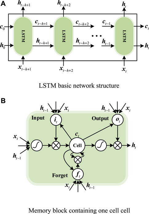
FIGURE 8. LSTM network architecture.

In the traditional one-way LSTM, the update of internal variables follows a strict one-way transfer rule, which leads to a one-way temporal dependence of the hidden states of the LSTM at each moment from the history to the future. As shown in Figure 8, the final state ${\mathit{h}}_t$ of the network is intrinsically related to $\left({\mathit{x}}_1,{\mathit{x}}_2,\cdots ,{\mathit{x}}_t\right)$ at all previous moments, while the hidden state ${\mathit{h}}_{t-1}$ at the previous moment cannot be linked to ${\mathit{x}}_t$. Therefore, in the one-way LSTM, only the final hidden state can utilize all the input information, while the hidden state of the previous moment cannot be influenced by the subsequent input information. For the load sequence, there is a close relationship between the historical moment’s load and the future moment’s load. The one-way LSTM is only capable of capturing the time dependence of the load sequence from the past to the future, and is unable to derive feature information in the reverse direction. This paper uses BiLSTM for temporal feature extraction of load sequences in order to resolve the inherent defects of one-way LSTM. Figure 9 depicts the structure of BiLSTM, which consists of both forward- and backward-facing one-way LSTMs. BiLSTM can be trained forward and backward. BiLSTM can fully utilize the input information and perform temporal feature extraction more comprehensively than one-way LSTM.

FIGURE 9

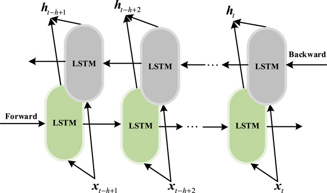
FIGURE 9. Bidirectional LSTM network structure.

As can be seen in Figure 9, the hidden state $\mathit{h}$ of the BiLSTM is determined by the forward LSTM and the inverse LSTM together as follows:

$\mathit{h}=\left[\overrightarrow{\mathit{h}}\oplus \stackrel{⃖}{\mathit{h}}\right](5)$

To summarize the previous analysis, it uses BiLSTM to capture the temporal dependencies of the fused load feature sequence $\mathit{R}$ obtained in subsection 3.2. The number of time steps of BiLSTM is $h$. The hidden state vector output from the last hidden layer of BiLSTM is shown as follows:

${\mathit{h}}_t=\left[h_t^1,h_t^2,\cdots ,h_t^n\right](6)$

In the formula: ${\mathit{h}}_t$ is the vector of hidden states output by BiLSTM; $h_t$ is a hidden state at time $t$; $n$ is the number of hidden states, which depends on the number of neurons in the top hidden layer of BiLSTM.

4 Attentional mechanisms and multitask learning

4.1 Multi-head attention mechanism

The attention mechanism can be viewed as a means of resource allocation in the model learning process, with the weight parameter of each feature serving as the resource of interest for the attention mechanism in deep neural networks. The attention mechanism focuses the model on important information by adaptively assigning weights to input variables. This paper proposes a multi-head attention mechanism model, as shown in Figure 10.

FIGURE 10

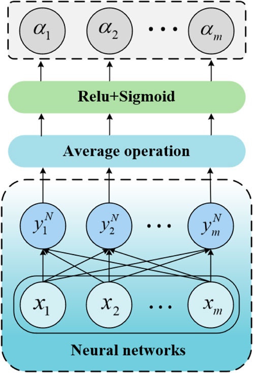
FIGURE 10. Multi-head attention mechanism.

Taking a set of input features $\mathit{X}=\left[x_1,x_2,\cdots ,x_M\right]$ of dimension $M$ as an example, a shared linear layer is used to obtain a preliminary weight vector $\mathit{Y}$, as shown below:

$\mathit{Y}=\mathit{\sigma }\left(\mathit{W}\mathit{X}+\mathit{b}\right)(7)$

Where, $\mathit{Y}=\left[y_1,y_2,\cdots ,y_M\right]$ denotes the initial weight coefficients of each input feature; $\mathit{W}$ is the weight matrix; $\mathit{b}$ is the bias matrix; $\mathit{\sigma }$ is the linear activation function.

On this basis, because this paper adopts the multi-head attention mechanism, a total of $N$ linear transformations are performed, and the preliminary weight vector obtained by the $N$-th linear transformation is ${\mathit{Y}}^{\left(N\right)}=\left[y_1^{\left(N\right)},y_2^{\left(N\right)},\cdots ,y_M^{\left(N\right)}\right]$, and then the $N$ preliminary weight vectors obtained are averaged to obtain the preliminary mean weight vector $\overline{\mathit{Y}}$ is:

$\overline{\mathit{Y}}=\frac{1}{N}{\displaystyle \sum _{S=1}^N}{Y}^{\left(S\right)}(8)$

The relu activation function is used to restrict the initial mean weight vector $\overline{\mathit{Y}}=\left[{\overline{y}}_1,{\overline{y}}_2,\cdots ,{\overline{y}}_M\right]$ to a non-negative interval, and then normalize the weight coefficients by the Sigmoid function to obtain the final attention weight coefficients $\mathit{\alpha }=\left[{\alpha }_1,{\alpha }_2,\cdots ,{\alpha }_M\right]$, as shown below:

$\mathit{\alpha }=sigmoid\left(relu\left(\left[{\overline{y}}_1,{\overline{y}}_2,\cdots ,{\overline{y}}_M\right]\right)\right)(9)$

In this paper, the initial mean weight vector $\overline{\mathit{Y}}$ is first one-sidedly suppressed to the positive interval by the Relu function, and then normalized using Sigmoid. Finally, the final obtained feature attention weight vector is multiplied with the original input feature vector by elemental correspondence to obtain the weighted input feature vector, as shown below:

${\mathit{X}}^{\prime }=\mathit{\alpha }\odot \mathit{X}=\left[{\alpha }_1{x}_1,{\alpha }_2{x}_2,\cdots ,{\alpha }_M{x}_M\right](10)$

In the formula: ${\mathit{X}}^{\prime }$ is the weighted eigenvector; $\odot$ is the Hadamard product.

4.1.1 Spatial attention

The most direct input feature of this paper is the load demand of each load unit at different moments in time, where the proportion of consumption of the three energy sources varies among load units and where a portion of the load units consume only one or two types of energy. Load pixel points that are irrelevant to a certain total load demand are not only unhelpful to the prediction result but even cause information interference in the model prediction. In this paper, the weights assigned to different load pixels can be calculated dynamically by introducing the spatial attention mechanism. The basic structure of the spatial attention mechanism model is shown in Figure 10, in which the input of the multi-head attention mechanism model is the pixel image of each load component constructed in subsection 3.1, and the output is the load pixel image after weighting each load pixel point. Due to the introduction of the spatial attention mechanism, the spatial attention weights can be used to express the contribution of different load pixels to each type of total load, so that the prediction model can focus on “important” load pixels in the learning process.

4.1.2 Temporal attention

Load forecasting is a typical time series forecasting problem, which is reflected in the extremely high dependence on historical information. In this paper, the temporal attention mechanism is introduced into the model to deeply mine the time series information. The basic structure of the temporal attention mechanism is shown in Figure 10, in which the input to the model of the multi-head attention mechanism is the fused load sequence at the standard time step in subsection 3.2. Attention weights are assigned to the fusion features under each time step by the temporal attention mechanism to increase the model’s attention to the important time point information during the training process.

4.2 Multitask learning mechanism

The data recorded by UIES contains a large amount of shared information about energy conversion. Multi-task learning can utilize this shared information to learn and acquire knowledge among multiple load prediction tasks and train the shared hidden layer on all tasks in parallel, thus improving the prediction accuracy of each load. In addition, the parameter sharing strategies for multi-task learning can be broadly categorized into hard and soft sharing (Niu et al., 2022). Considering the strong coupling of each load in UIES, this paper chooses the hard sharing mechanism that is suitable for dealing with more strongly correlated tasks. The structure of the hard sharing mechanism for multi-task learning is shown in Figure 11.

FIGURE 11

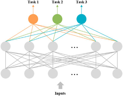
FIGURE 11. Multi-task learning network structure based on hard sharing mechanism.

For a multi-task learning under a hard sharing mechanism, which contains multiple learning tasks ${\mathit{y}}^m\left(m\in M\right)$ and data sets $\left\{{\mathit{x}}_i,y_i^1,y_i^2,\cdots ,y_i^M\right\}$, $\left(i=\mathrm{1,2},\cdots ,N\right)$, where $M$ is the number of tasks, $N$ is the number of data samples, and $y_i^m$ is the $m$-th task label of the $i$-th data point. $f^m\left(\mathit{x};{\mathit{\theta }}^{sh},{\mathit{\theta }}^{ea}\right)$, $\mathit{x}\to {\mathit{y}}^m$ is the prediction function, where ${\mathit{\theta }}^{sh}$ is the shared parameter of each task in the shared layer, and ${\mathit{\theta }}^{ea}$ is the independent correlation parameter of each task itself. Under multi-task learning, the overall objective optimization loss function is defined as:

$\left\{\begin{array}{l}L\left(\mathit{\theta }\right)=\mathit{min}{\displaystyle \sum _{m=1}^M}{\lambda }^m{\widehat{L}}^m\left({\mathit{\theta }}^{sh},{\mathit{\theta }}^{ea}\right)\\ {\widehat{L}}^m\left({\mathit{\theta }}^{sh},{\mathit{\theta }}^{ea}\right)=\frac{1}{N}{\displaystyle \sum _{i=1}^N}{\widehat{L}}^m\left(f^m\left({\mathit{x}}_i;{\mathit{\theta }}^{sh},{\mathit{\theta }}^{ea}\right),y_i^m\right)\end{array}\right.(11)$

In the formula: ${\lambda }^m$ is the weight coefficient of each task; ${\widehat{L}}^m\left({\mathit{\theta }}^{sh},{\mathit{\theta }}^{ea}\right)$ is the loss function; $L\left(\mathit{\theta }\right)$ is the overall objective optimization loss function.

5 IES multiple load prediction framework based on spatio-temporal coupling and multi-headed attention

The forecasting workflow in this paper is divided into the following six stages:

Step 1. Load pixel image construction

Based on the load pixel image construction method in subsection 3.1, a comprehensive load pixel image containing three load components of electricity, heat, and cold is constructed at a certain moment, as shown below.

$\mathit{P}=\left[\left[\begin{array}{ccc}{p}_{\mathrm{1,1}}^e& \cdots & p_{1,n}^e\\ ⋮& \ddots & ⋮\\ p_{n,1}^e& \cdots & p_{n,n}^e\end{array}\right],\left[\begin{array}{ccc}{p}_{\mathrm{1,1}}^h& \cdots & p_{1,n}^h\\ ⋮& \ddots & ⋮\\ p_{n,1}^h& \cdots & p_{n,n}^h\end{array}\right],\left[\begin{array}{ccc}{p}_{\mathrm{1,1}}^c& \cdots & p_{1,n}^c\\ ⋮& \ddots & ⋮\\ p_{n,1}^c& \cdots & p_{n,n}^c\end{array}\right]\right](12)$

In the formula: $\mathit{P}$ is the integrated load pixel image at a certain time section; $p^e$, $p^h$, and $p^c$ represent the electric load, hot load, and cooling load pixel points respectively; $n\times n$ is the size of the load pixel image, which can also be regarded as the resolution size.

Based on this, the integrated load pixel images at different historical moments from the prediction target moment $\left(t+1\right)$ need to be constructed separately. Further, the time-varying nature of the load is demonstrated by a frame by frame load pixel image, and the pixel values at any specific location will be continuously updated according to a certain temporal resolution, as shown in equation 13. The dimension size of the input features is thus $n\times n\times 3h$, where $n$ is the spatial dimension, $h$ is the channel dimension, which is the length of the historical time period.

$\mathit{G}=\left[{\mathit{P}}_{t-h+1},{\mathit{P}}_{t-h+2},\cdots ,{\mathit{P}}_t\right](13)$

Step 2. Spatial attention weighting

Before inputting each load component pixel image into MCNN for spatial feature extraction, the spatial attention layer is constructed using the multi-head attention mechanism proposed in subsection 4.1 of this paper. The input features’ spatial dimension is first reduced to their channel dimension, and the input feature dimension becomes $1\times 1\times 3nnh$, which is then input to multiple shared linear layers. The dynamic assignment of spatial attention weights during model learning is realized according to equation 7 to equation 10, and each load pixel point is assigned its own spatial attention weight coefficient. Finally, the attention weight vector is dimensionally recovered as $n\times n\times 3h$, and multiply it with the corresponding load pixel points of the original load pixel image to obtain a weighted load pixel image ${\mathit{G}}^{\prime }$.

${\mathit{G}}^{\prime }=\left[{\mathit{\alpha }}_{t-h+1}{\mathit{P}}_{t-h+1},{\mathit{\alpha }}_{t-h+2}{\mathit{P}}_{t-h+2},\cdots ,{\mathit{\alpha }}_t{\mathit{P}}_t\right](14)$

$\mathit{\alpha }\mathit{P}=\left[\begin{array}{ccc}{\alpha }_{\mathrm{1,1}}{p}_{\mathrm{1,1}}^e& \cdots & {\alpha }_{1,n}{p}_{\mathrm{1,1}}^e\\ ⋮& \ddots & ⋮\\ {\alpha }_{n,1}{p}_{n,1}^e& \cdots & {\alpha }_{n,n}{p}_{n,n}^e\end{array}\right](15)$

In the formula: $\mathit{\alpha }$ is the attention weight vector of the integrated load pixel image at a certain moment; $\alpha$ is the attention weight coefficient of a load pixel point.

Step 3. Spatial feature extraction and fusion

On the basis of step 2, this paper inputs the weighted pixel images of each load component into the MCNN neural network architecture constructed in subsection 3.2 for spatial feature extraction and fusion.

Step 4. Temporal attention weighting

Before inputting the fused load time series obtained from step 3 into the BiLSTM shared layer, the temporal attention layer is constructed using the multi-head attention mechanism proposed in subsection 4.1. First, the fusion load feature vectors under each time step are sequentially input into multiple shared linear layers, and the feature vectors under each time step are dynamically assigned with temporal attention weight coefficients based on equations 7 to 10. Finally, the weighted fusion load time series is obtained by multiplying the temporal attention weight vector with the feature vectors under each time step by element. This is shown in the following equation:

$\mathit{R}=\left[{\mathit{\beta }}_{t-h+1}{\mathit{F}}_{t-h+1},{\mathit{\beta }}_{t-h+2}{\mathit{F}}_{t-h+2},\cdots ,{\mathit{\beta }}_t{\mathit{F}}_t\right](16)$

In the formula: $\mathit{\beta }$ is the temporal attention weight vector at a certain moment.

Step 5. Time-dependent relationship capture

The weighted fused load time series obtained from step4 is input to BiLSTM feature sharing layer for bidirectional temporal information mining to extract temporal feature information.

Step 6. Multi-task learning joint prediction

In this paper, a multi-task learning approach based on a hard-sharing mechanism is used for joint forecasting of electricity, heat, and cold loads. In this, the parameters of BiLSTM as the bottom layer are uniformly shared, and the parameters of each fully connected layer as the top layer are independent of each other. Due to different physical dynamics and different energy demand characteristics, the various types of loads have different fluctuation frequencies. In the UIES studied in this paper, the electric and thermal load profiles have large local fluctuations with rich details, while the cooling load profile is relatively smooth. The same feature interpretation network (the same top layer structure) cannot simultaneously portray the fluctuation characteristics of each load curve, and it is difficult to make the three kinds of loads achieve a better fitting state at the same time. Therefore, it is necessary to construct independent, fully connected neural network (FCNN) for the three loads as the feature interpretation network.

According to the analyses in subsections 2.1 and 2.2, it can be seen that the actual load changes have obvious correlations with meteorological factors and calendar rules. In the calendar rule, hourly, day-type information as well as holiday information are incorporated. The meteorological factors are selected as temperature, dew point, irradiance, and humidity. The calendar rules and meteorological factors as external input features are extracted through three fully connected layers and spliced with the output features of BiLSTM, which are input to the top inputs of electric, heat, and cold loads, respectively, to fully explore the dependence of each load on the calendar and meteorological information.

${\mathit{h}}_t^{\prime }=\left[h_t^1,h_t^2,\cdots ,h_t^n,{\mathit{c}}_t,{\mathit{d}}_{t+1}\right](17)$

In the formula: ${\mathit{h}}_t^{\prime }$ is the extended feature vector; ${\mathit{c}}_t$ is the vector of meteorological information under the historical moment preceding the moment to be predicted; ${\mathit{d}}_{t+1}$ is a vector of calendar information under the moment to be predicted.

As shown in Figure 12, the user-level IES multivariate load prediction framework based on multi-energy spatio-temporal coupling and spatio-temporal attention mechanism, which is a neural network framework with deep spatio-temporal correlation, has been fully completed.

FIGURE 12

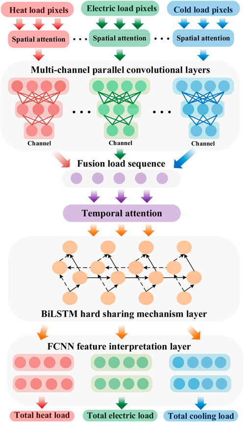
FIGURE 12. UIES multivariate load forecasting framework.

6 Experiment setup and result analysis

6.1 Introduction to data sources

The data source for this paper is the user-level IES at Arizona State University’s Tempe campus, which is located in a tropical desert climate with high demand for cooling and electrical loads and low demand for heat loads, and a large portion of the cooling loads come from electric cooling equipment in the IES system. Electricity, heat, and cooling load data (including all types of load data for 115 load units and all types of total load data) recorded by the university’s Campus Metabolism project web platform from January 2019 to March 2020 were used, with a time resolution of 1 h. Based on the forecasting framework in Figure 12, the total electrical, thermal, and cooling loads for the next 1 h for this IES system are forecasted. Before constructing the input feature set, considering that there are some missing and anomalous mutations in the data stored in this UIES, this paper firstly replaces and supplements the anomalies and vacancies, and normalizes the original data to the interval [0,1] according to the following formula for model training.

$x_{\omega }=\frac{x_{\phi }-x_{\mathit{min}}}{x_{\mathit{max}}-x_{\mathit{min}}}(18)$

In the formula: $x_{\omega }$ is the normalized value of a load in a basic energy consumption unit; $x_{\phi }$ is the actual value with a dimension; $x_{\mathit{min}}$ and $x_{\mathit{max}}$ are the minimum and maximum values.

In this paper, each load unit is classified according to its functional attributes, of which 24 are teaching venues, 15 are scientific research venues, 13 are administrative venues, 4 are art venues, 11 are sports venues, 29 are residential venues, 11 are public activity venues, and 8 are other auxiliary venues. On this basis, the load component pixel images under different moments of size $11\times 11$ are constructed according to subsection 3.1.

The determination of the length of the historical time period $h$ is considered to take into account two aspects, which are the difficulty of model training and the completeness of the knowledge embedded in the input features. If $h$ is too small, there will be insufficient knowledge in the historical sequence for the model to learn, thus limiting the prediction accuracy and generalization ability of the model. Conversely, if $h$ is too large by considering only the completeness of knowledge information in the historical sequence, it will increase the complexity of model training and thus affect the optimization of model parameters. Therefore, the value of $h$ needs to balance the above two aspects. Combined with the analysis in subsection 2.3 and through a large number of experimental comparisons, the length of $h$ is finally determined to be 9. The historical data of $t+1$ moments a week ago and a day ago, as well as the historical data of the first seven historical moments ($t-6$ to $t$) near the forecast target moment, are taken as the reference for the current load forecast at $t+1$ moments. As a result, the dimension size of the input features of the prediction model constructed in this paper is $11\times 11\times 27$.

A pixel image of the electrical load at 3 consecutive moments is shown as an example, as shown in Figure 13 (load is normalized value). Since the temporal resolution is 1 h, the variation of the electrical load can be represented as a frame by frame picture at 1 h intervals.

FIGURE 13

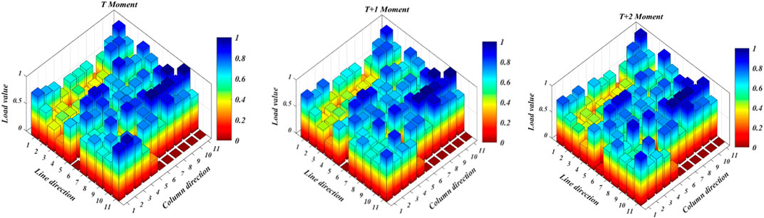
FIGURE 13. Pixel images of the electrical load at different moments.

6.2 Basic evaluation indicators

In this paper, the mean absolute percentage error (MAPE) and root mean square error (RMSE) metrics are selected to evaluate the forecasting effectiveness of each load, and the expressions are:

$RMSE=\sqrt{{\displaystyle \sum _{\theta =1}^M}\frac{{\left(Y\left(\theta \right)-\widehat{Y}\left(\theta \right)\right)}^2}{M}}(19)$

$MAPE=\frac{1}{M}{\displaystyle \sum _{\theta =1}^M}\left|\frac{Y\left(\theta \right)-\widehat{Y}\left(\theta \right)}{Y\left(\theta \right)}\right|\times 100\%(20)$

In the formula: $\widehat{Y}\left(\theta \right)$ is the predicted value of load at the $\theta$ -th sampling point; $Y\left(\theta \right)$ is the actual value of load at the $\theta$ -th sampling point; $M$ is the number of test samples.

In addition, in order to evaluate the performance of the multivariate load forecasting model as a whole, this paper considers the importance of different loads in the system, assigns different importance weights to different loads, and evaluates the overall forecasting effect of the model by using the mean absolute percentage error of multiple weights (WMAPE). Since the proportion of cold and electric loads in UIES is high and the proportion of heat loads is low, the weights of cold loads, heat loads and electric loads are set to 0.4, 0.2 and 0.4, respectively. The expressions of specific evaluation indexes are as follows.

$\left\{\begin{array}{l}WMAPE={\displaystyle \sum _{k=1}^N}{R}_{k}MAPE\left(k\right)\\ {\displaystyle \sum _{k=1}^N}{R}_k=1\end{array}\right.(21)$

In the formula: $WMAPE$ is the mean absolute percentage error of the integrated load; $R_k$ is the importance weight of the $k$ -th type of load; $N$ is the number of load types.

6.3 Model hyperparameter settings

For the MCNN network proposed in this paper, it is known from subsection 6.1 that its input feature set is an electrical, thermal, and cold load pixel image of size $11\times 11$ at 9 moments, so the dimensional size of the MCNN input features is $11\times 11\times 27$. Based on the analysis in subsection 3.2, the number of channels of MCNN is determined to be 27, and each channel has a 4-layer independent structure with only convolutional layer and no pooling layer, and the convolutional kernel sliding step is 1, and no Padding operation is performed. First, the first convolution layer of each channel consists of eight convolution kernels of size $5\times 5$, thus covering a larger number of loaded pixel points in the spatial association domain, so that each pixel point in the generated feature map can obtain a large perceptual field. Second, the size of the convolutional kernels in the second to fourth layers is $3\times 3$ and the number of convolutional kernels increases in the order of 16, 32, and 64. Finally, the size of each feature map output by MCNN is $1\times 1$, and its perceptual field size in theory is the original input load pixel image, which contains global information, and the number of feature maps is $27\times 64$. Based on this, we again use the multi-channel idea to set up 9 channels, each with a convolutional kernel size of $1\times 1$ and a number of 64. After one convolution operation, the spatial features of electric, thermal and cooling loads under the same time section are fused to form a time series of fused load features at standard time steps.

The number of neurons and hidden layers are the two critical hyperparameters for BiLSTM. In the study findings of recurrent neural networks represented by LSTM used to load prediction, the majority of them are empirically compared and eventually set the number of hidden layers in the network from 1 to 5, with the number of neurons in each hidden layer often not exceeding 200. BiLSTM has been observed to frequently experience overfitting, which lowers prediction accuracy when the number of hidden layers or the number of neurons in the hidden layers is excessive. In this study, we carried out a number of tests and discovered that BiLSTM functions best when there are two hidden layers and an increase in the number of neurons in each layer on the order of 64,128.

For the three different structures of feature interpretation modules, the fully connected layer for cold loads is designed as one layer with 16 neurons. The fully connected layer for electrical loads is designed as two layers with 32 and 16 neurons per layer, respectively. The fully connected layer for thermal load is designed as 3 layers with 64, 32, and 16 neurons per layer, respectively.

The Adam algorithm is chosen to train the network with a learning rate of 0.01 within this paper, a batch size of 256, and an iteration number of 100. To prevent overfitting, a droup-out operation is added to the training process, and the probability parameter is kept at 0.9. The model is developed in the Keras deep learning framework. The hyperparameter configuration of the model is shown in Table 1.

TABLE 1

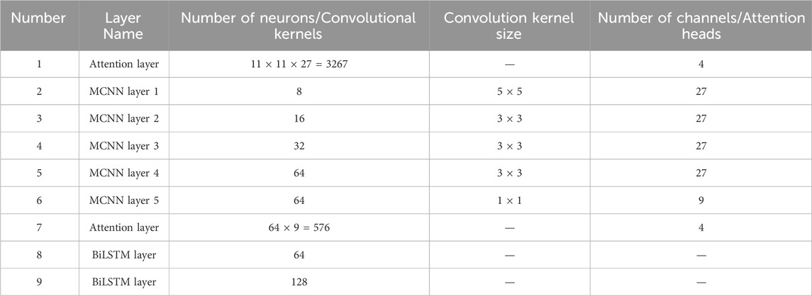
TABLE 1. Network hyperparameter settings.

6.4 Comparative analysis of prediction results

In order to fully validate the effectiveness of the IES multivariate load prediction framework (Case 7) proposed in this paper, six contrasting models are set up in this section. Among them, Case1 to Case3 are predicted by multi-task learning, and Case4 to Case6 are predicted by single-task learning. Among them, the multi-task learning models all consider the coupling characteristics of each load, while the single-task learning models do not consider the coupling characteristics of each load.

Case 1. Based on Case 7, the spatial features are extracted using MCNN without considering the feature independence of each load, and only the temporal integrity is preserved. The number of channels of MCNN is 9, and the input feature of each channel is the integrated load pixel image at the corresponding moment. The hyperparameters of MCNN, BiLSTM and spatio-temporal attention layer are the same as Case 7 except that there is no feature fusion operation based on MCNN. Multi-task learning is used to simultaneously predict the total electric, cooling and heating loads at the next moment.

Case 2. The input and output feature sets, model structure and hyperparameters are the same as Case7, except that the attention mechanism is not used, and Case2 considers feature independence and temporal integrity of each load during feature extraction.

Case 3. The historical values of the total electrical, thermal and cooling loads are used as input features and then BiLSTM is used as a feature sharing layer for joint prediction of each of the total loads by multi-task learning. The hyperparameters of BiLSTM are the same as those of Case7’s BiLSTM.

Case 4. Based on Case7, the coupling characteristics of each load are not considered. The number of input channels of MCNN is 9, and the input feature of each channel is the pixel image of a certain type of load component at the corresponding moment. The hyperparameters of MCNN, BiLSTM and spatio-temporal attention layer are the same as Case7 except that there is no feature fusion operation based on MCNN. The total load of each category at the next moment is predicted independently using single-task learning.

Case 5. Same as Case4, but without the spatio-temporal attention layer based on the multiple attention mechanism.

Case 6. Based on Case 3, the total electrical, thermal, and cooling loads are predicted separately and independently using single-task learning without using multi-task learning. The input features are the historical values of a particular total load itself, and the hyperparameter configuration is the same as in Case3.

Considering that the energy consumption patterns of this UIES in summer and winter are quite different, the external morphological characteristics presented by each load show a large change. Therefore, in this paper, the comparison experiments are designed by selecting the data for each load for a week in winter and summer, respectively. Figure 14; Figure 15 show the prediction results of electric, thermal, and cooling loads for 1 week in different seasons, and Table 2, Table 3 show the prediction errors for each case in the test set.

FIGURE 14

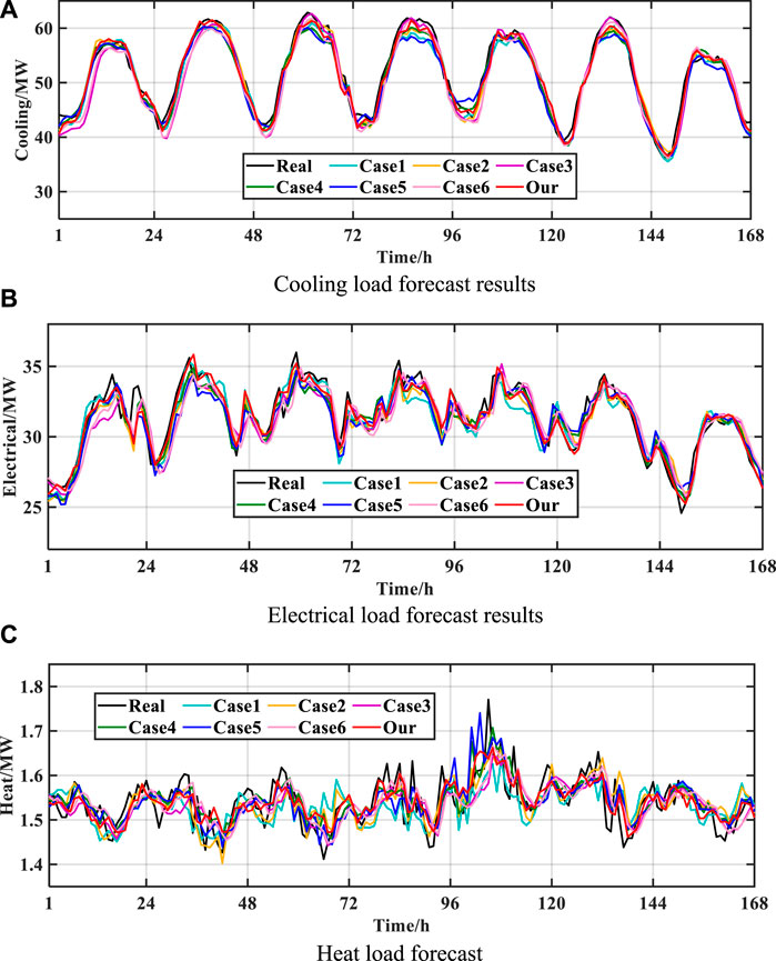
FIGURE 14. Results of each load forecast in summer. (A) Cooling load forecast results. (B) Electrical load forecast results. (C) Heat load forecast.

FIGURE 15

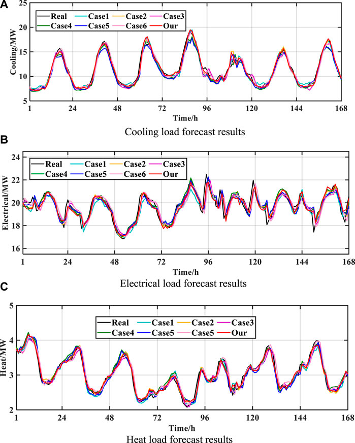
FIGURE 15. Results of each load forecast in winter. . (A) Cooling load forecast results. (B) Electrical load forecast results. (C) Heat load forecast.

TABLE 2

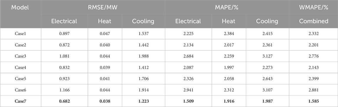
TABLE 2. Evaluation index of prediction effect of each model in summer.

TABLE 3

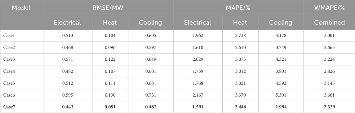
TABLE 3. Evaluation index of prediction effect of each model in winter.

6.4.1 Analysis of the effect of cold load prediction

The results of the cold load forecasts under the summer and winter time periods are shown in Figure 14A and Figure 15A, respectively. It is easy to see that the cold load demand size under the two seasons has a large change. In the summer season, the daily cold load change has obvious regularity, and the forecast models can track the load change trend better. In winter, the cooling load curves shown in the 96th to 120th hour change significantly compared with the other hours, and it can be seen that the prediction error in this hour is much larger than the other hours.

(1) Analysis of the effectiveness of multitask learning models for cold load prediction

In the summer, as shown in Table 2, the prediction accuracies of Case 1, Case 2, and Case 7 are higher than those of Case 3, which indicates that, compared with BiLSTM based on macroscopic class load prediction methods, the microscopic class load prediction method can learn the intrinsic law of change of the loads better, which is attributed to the rich information embedded in its input features. Compared with Case 1, the RMSE of Case 2 is reduced by 6.18%, and the MAPE is reduced by 2.23%. This indicates that even with the introduction of the attention mechanism in Case 1, better prediction results can still be achieved by taking into account the independent characteristics of the loads themselves in the feature extraction process. Compared with Case 2, the RMSE of Case 7 is reduced by 15.18%, and the MAPE is reduced by 15.84%.

As shown in Table 3, the prediction accuracy of the models on cooling loads during the winter time period is ranked as Case7>Case2>Case1>Case3. The RMSE of Case 1 is reduced by 6.77 percent, and the MAPE is reduced by 3.31 percent as compared to Case 3. Case 2 had a 1.32% lower RMSE and 10.26% lower MAPE compared to Case 1. RMSE was reduced by 19.26% and MAPE was reduced by 20.13% for Case 7 compared to Case 2.

(2) Analysis of the effectiveness of single-task learning models for cold load prediction

The prediction accuracies of the models for the two seasons with respect to the cooling loads were ranked as Case 4 > Case 5 > Case 6. The RMSE and MAPE of Case4 were 17.23% and 10.67% lower in the summer time period, respectively, as compared to Case5. Under the winter time period, Case 4 had 11.74% lower RMSE and 17.22% lower MAPE than Case 5. This indicates that the introduction of the attention mechanism can strengthen the significant features of the loaded pixel images and fused load sequences so as to obtain more important feature information in the feature extraction process and improve the prediction accuracy of the model.

(3) Multi-task learning model VS. Single-task learning model

During the summer time period, Case 2 had the best prediction performance among the multi-task models except Case 7. Among the single-task models, the highest prediction accuracy is achieved by Case 4. Compared to Case 2, Case 4 has a 2.08% lower RMSE and a 3.72% lower MAPE. This is because the summer cold load fluctuation is more regular, and only relying on its own load pixels is enough for the model to learn its own intrinsic pattern of change, while the attention mechanism introduced in Case 4 further improves the model performance.

In the winter time period, the prediction accuracy of Case2 is slightly higher than that of Case4, and its RMSE is reduced by 0.66% and MAPE is reduced by 1.36% compared with Case4. This is because the cold load’s volatility is strengthened at this time, and relying only on its own load pixel does not allow the model to learn the intrinsic correlation between the cold load and other loads, which weakens the model’s ability to perceive the fluctuation pattern of the cold load itself. In addition, the introduction of the attention mechanism in Case 4 compensates for the defect of limited information expressed by input features to a certain extent.

6.4.2 Analysis of the effect of electrical load prediction

The predicted electric loads for the summer and winter periods are shown in Figure 14B and Figure 15B, respectively. Combining Figure 14A and Figure 15A, it can be seen that the electric load fluctuates more than the cold load, which is especially obvious in the winter, and the prediction curves of Case1 deviate more from the actual curves in some time periods, while the prediction curves of Case7 follow the actual load curves in the best way. Compared with the cold load forecasting task, the models show more obvious performance differences in electrical load forecasting.

(1) Analysis of the effectiveness of multitask learning models for electrical load prediction

As shown in Table 2, the RMSE of Case 1 decreased by 17.02% and the MAPE decreased by 17.10% compared to Case 3. The reason for the difference in the performance of the two models is that the input features of Case 3 only include the historical data of each total load, which covers limited information and does not allow the model to fully learn the fluctuation pattern of each load. Compared with Case 1, the RMSE of Case 2 decreased by 2.78% and the MAPE decreased by 4.08%. This again shows that it is important to maintain the independence of each load in the feature extraction process. In addition, the RMSE of Case 7 decreased by 21.78% and the MAPE decreased by 29.28% compared to Case 2. This again demonstrates that the attention mechanism improves the model learning performance.

As can be seen from Table 3, Case 3 had the lowest prediction accuracy. The RMSE and MAPE of Case1 were reduced by 10.15% and 3.30%, respectively, compared to Case3. The RMSE and MAPE of Case 2 were reduced by 18.03% and 20.65%, respectively, compared to Case 3. The RMSE and MAPE of Case 2 were 8.77% and 17.94% lower than Case 1, respectively. The more drastic load fluctuations in the winter compared to the summer lead to a further increase in the performance difference between Case1 and Case2 on the load forecasting task. The RMSE and MAPE of Case 7 are only 5.34% and 1.12% lower than those of Case 2, respectively. This is due to the high volatility of electrical loads in winter, resulting in the introduction of an attentional mechanism that does not have a significant improvement effect.

(2) Analysis of the effectiveness of single-task learning models for electrical load prediction

The ranking of the accuracy of the models on the task of electrical load forecasting under two seasons is Case4>Case5>Case6. In the summer time period, RMSE for Case 4 was 9.85% lower than Case 5, and MAPE was 10.27% lower than Case 5. In the winter, the RMSE and MAPE of Case 4 were only 5.85% and 0.51% lower than those of Case 5, respectively.

(3) Multi-task learning model VS. Single-task learning model

The RMSE and MAPE of Case4 are 4.58% and 2.20% lower than those of Case2 on the electric load forecasting task in the summer time period, respectively. This indicates that the introduction of the attention mechanism focusing on the electric load’s own load pixels is better than mining the potential correlations among loads based on various types of load pixels. In contrast, under the winter time period, the RMSE for Case 2 is 2.90% lower than Case 4, and the MAPE is 8.47% lower than Case 4. The reason for analysing the above results is the same as that of the cold load forecasting task, which is because the cold loads in this UIES are mainly from electric loads, and the trend of electric load changes is largely consistent with the cold loads.

6.4.3 Analysis of the effect of heat load prediction

The heat load prediction results under the summer and winter time periods are shown in Figure 14C and Figure 15C, respectively. Among them, winter is a typical heat-consuming season for thermal systems, and the heat load demand decreases abruptly during the day and increases at night with obvious regularity. Each model can track the actual fluctuation changes of heat load better. For summer, the user heat demand is small and the heat behavior is random, which directly leads to the heat load fluctuation being extremely violent, the rule of change is not traceable. The prediction results of each model can’t fit the actual curve of heat load well, and some of the prediction results of Case 1 and Case 5 have a big deviation from the actual value.

(1) Analysis of the effectiveness of multitask learning models for heat load prediction

The prediction accuracies of the models on the task of heat load prediction in summer are Case7>Case2>Case3>Case1. Compared to Case 1, Case 3 has a 6.38% lower RMSE and a 5.24% lower MAPE. Due to the extremely random variation of heat load, its correlation with electricity and cooling load is small. Meanwhile, Case 1 does not consider the independent characteristics of each load in feature extraction, which increases the difficulty of the model learning the fluctuation law of heat load, resulting in poor heat load feature extraction. This point also illustrates the effectiveness and reasonableness of Case7 and Case2 in constructing feature extraction channels independently for each load component pixel image. Case 3 predicts the heat load based on its own historical data and achieves better prediction results than Case 1.

The prediction accuracies of the models on the heat load prediction task in winter time are Case7>Case2>Case1>Case3, and the RMSE and MAPE of Case2 are only 7.69% and 4.32% lower than those of Case1 and Case2, respectively. This is because the correlation between the heat load and the electricity and cooling loads is stronger at this time, and the simultaneous feature extraction of the pixel images of each load component at the same moment in time does not have much effect on the learning effect of the model. Compared with Case 2, the RMSE and MAPE of Case 7 are only reduced by 5.21% and 6.28%, respectively. This is because the heat load fluctuation pattern is obvious, and the model can extract the heat load feature information better, resulting in the improvement effect of the attention mechanism that is not obvious.

(2) Analysis of the effectiveness of single-task learning models for heat load prediction

The prediction accuracies of the models on the heat load prediction task in the two seasons are ranked as Case 4 > Case 5 > Case6. In the summer, the RMSE of Case4 and Case5 are reduced by 11.36% and 6.81%, respectively, and the MAPE is reduced by 13.62% and 10.98%, respectively, compared with Case6. Case4 and Case5 extract features from the heat load pixels, which can learn the complex fluctuation patterns within the heat load in a more detailed way and are more advantageous than mining feature information directly from the heat load’s own historical data. In winter time, compared with Case6, the RMSE of Case4 and Case5 are reduced by 17.69% and 14.61%, respectively, and the MAPE is reduced by 10.62% and 10.35%.

(3) Multi-task learning model VS. Single-task learning model

During the summer, the RMSE and MAPE of Case 4 were only 2.50% and 0.99% lower than Case 2, respectively. And the RMSE and MAPE of Case 7 were only 2.56% and 4.05% lower than Case 4, respectively. This shows that there is no valid information associated with the change of heat load in the pixel images of electric and cold loads, and also verifies that the idea of independent feature extraction for each load component pixel image in the front-end and fusion of each load feature at the same moment in the back-end proposed in this paper is correct. During the winter season, RMSE decreased by 10.28% and MAPE decreased by 13.34% in Case 2 compared to Case 4, and RMSE decreased by 5.21% and MAPE decreased by 6.28% in Case 7 compared to Case 2. This indicates that at this time there are signals in the electrical and cold load pixel images that are related to changes in the heat load, which helps to improve the feature extraction of the heat load.

6.4.4 The strengths analysis of the model

The data shown in Tables 4 and 5 indicate that Case 7 exhibits the best level of prediction accuracy for each load when compared to the other models. This is due to the fact that the proposed method in this paper is able to predict the multivariate loads of the UIES in a refined and three-dimensional way by load types and spatial and temporal characteristics. Case7 performs independent feature extraction on the pixel images of each load component at different moments and fuses the spatial features of the loads in the high-dimensional space, which takes into full consideration the independence of the features of the loads. The end-to-end information flow delivery of spatial feature extraction and time-dependent relationship capture is also realized. In addition, a multi-head attention mechanism is introduced to assign weight coefficients to load pixels and fused load features, respectively, which realizes the model’s differentiated attention among different features. Finally, multi-task learning is utilised for joint prediction of each load, which further exploits the coupling characteristics among loads. Through the close cooperation of the above three links, the advantages of each module are fully utilised, and more accurate prediction results are achieved.

TABLE 4

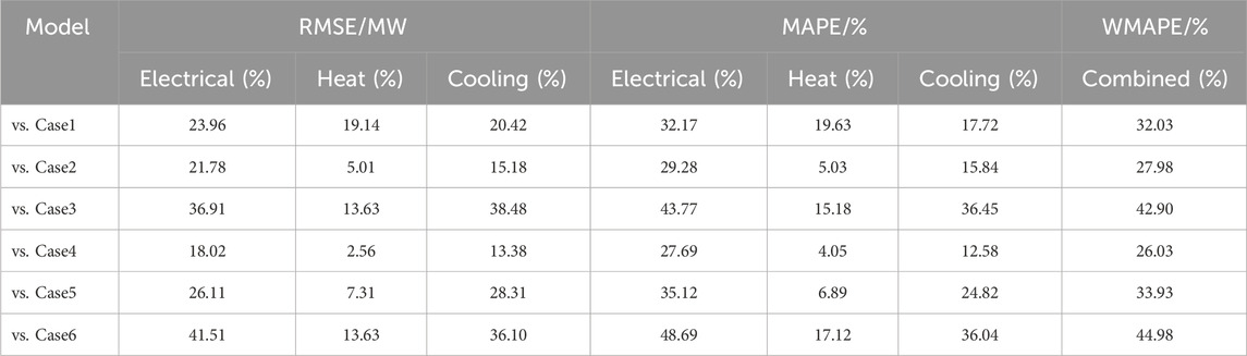
TABLE 4. Comparative analysis of the proposed model Case7 with other models in terms of forecasting accuracy of each load in summer season.

TABLE 5

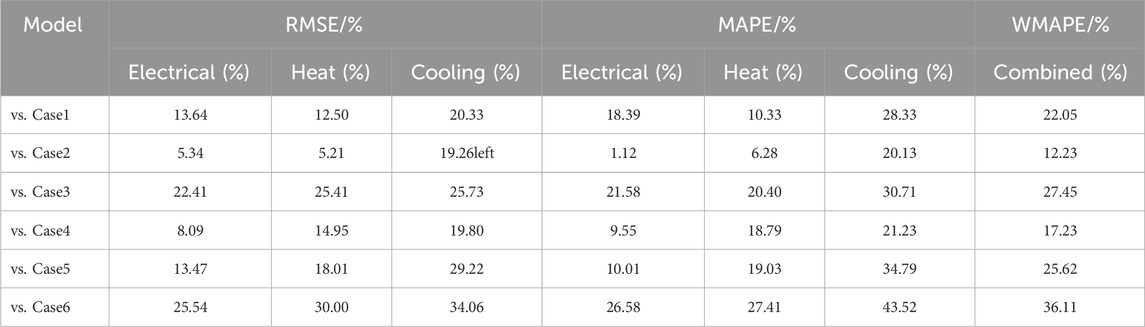
TABLE 5. Comparative analysis of the proposed model Case7 with other models in terms of forecasting accuracy of each load in winter season.

7 Conclusion

In this paper, a MCNN-BiLSTM load prediction method considering multi-energy spatio-temporal correlation is proposed for small-scale UIES, which realizes the stereoscopic feature extraction of UIES multivariate load spatio-temporal information. The following conclusions are obtained:

(1) The load units covered by the user-level IES hide the multidimensional information of various types of total loads, for which the input feature set in the form of an image is built, and with the powerful feature extraction capability of CNN, the prediction error caused by load uncertainty can be significantly reduced.

(2) There are many types of user-level IES loads with high volatility and complex correlations among loads. When feature extraction is performed for each load, the independence of each load needs to be fully considered, which could lead to more accurate results.

(3) Through the experimental comparative analysis, the introduction of the attention mechanism layer can assist the model in better mining the intrinsic law of change of each load, which improves the load prediction accuracy to a certain extent.

Along with the rise of digital twin technology, the energy system will develop in the direction of intelligence and digitalization. In the future, data-driven load forecasting methods will be widely used in integrated energy systems at all levels. How to combine macroscopic class load forecasting methods with microscopic class load forecasting methods, give full play to their respective advantages, and apply them to IES load forecasting is our next work plan.

Data availability statement

Publicly available datasets were analyzed in this study. This data can be found here: http://cm.asu.edu.

Author contributions

XY: Conceptualization, Data curation, Formal Analysis, Investigation, Methodology, Visualization, Writing–original draft, Writing–review and editing. ZG: Funding acquisition, Resources, Software, Supervision, Writing–original draft. YC: Conceptualization, Data curation, Visualization, Writing–review and editing. YH: Data curation, Writing–original draft. ZY: Funding acquisition, Resources, Writing–original draft.

Funding

The author(s) declare financial support was received for the research, authorship, and/or publication of this article. This work was supported by the National Natural Science Foundation of China (62273215) and the Natural Science Foundation of Shandong Province (ZR2020MF071).

Conflict of interest

The authors declare that the research was conducted in the absence of any commercial or financial relationships that could be construed as a potential conflict of interest.

Publisher’s note

All claims expressed in this article are solely those of the authors and do not necessarily represent those of their affiliated organizations, or those of the publisher, the editors and the reviewers. Any product that may be evaluated in this article, or claim that may be made by its manufacturer, is not guaranteed or endorsed by the publisher.

References

Al-Musaylh, M. S., Al-Daffaie, K., and Prasad, R. (2021). Gas consumption demand forecasting with empirical wavelet transform based machine learning model: a case study. Int. J. Energy Res. 45 (10), 15124–15138. doi:10.1002/er.6788

CrossRef Full Text | Google Scholar

Bai, B. Q., Liu, J. T., Wang, X., et al. (2022). Short-term forecasting of urban energy multiple loads based on MRMR and dual attention mechanism. Power Syst. Autom. 46 (17), 44–55.

Google Scholar

Cheng, H. Z., Hu, X., Wang, Li., et al. (2019b). A review of research on regional integrated energy system planning. Power Syst. Autom. 43 (07), 2–13.

Google Scholar

Cheng, Y. H., Zhang, N., Lu, Z. X., and Kang, C. (2019a). Planning multiple energy systems toward low-carbon society: a decentralized approach. IEEE Trans. Smart Grid 10 (5), 4859–4869. doi:10.1109/TSG.2018.2870323

CrossRef Full Text | Google Scholar

Fan, C., Xiao, F., and Zhao, Y. (2017). A short-term building cooling load prediction method using deep learning algorithms. Appl. energy 195, 222–233. doi:10.1016/j.apenergy.2017.03.064

CrossRef Full Text | Google Scholar

Gao, Z. K., Yu, J. Q., Zhao, A. J., Hu, Q., and Yang, S. (2022b). A hybrid method of cooling load forecasting for large commercial building based on extreme learning machine. Energy 238, 122073. doi:10.1016/j.energy.2021.122073

CrossRef Full Text | Google Scholar

Gao, Z. Z., Yin, X. C., Zhao, F. Z., Meng, H., Hao, Y., and Yu, M. (2022a). A two-layer SSA-XGBoost-MLR continuous multi-day peak load forecasting method based on hybrid aggregated two-phase decomposition. Energy Rep. 8, 12426–12441. doi:10.1016/j.egyr.2022.09.008

CrossRef Full Text | Google Scholar

Hu, X., Shang, C., Chen, D. W., et al. (2019). Multi-objective planning method for regional integrated energy systems considering energy quality. Automation Electr. Power Syst. 43 (19), 22–31.

Google Scholar

Ji, L., Zhang, B. B., Huang, G. H., Xie, Y. L., and Niu, D. X. (2018). GHG-mitigation oriented and coal-consumption constrained inexact robust model for regional energy structure adjustment -A case study for jiangsu province China. Renew. Energy 123, 549–562. doi:10.1016/j.renene.2018.02.059

CrossRef Full Text | Google Scholar

Li, C., Li, G., Wang, K. Y., and Han, B. (2022). A multi-energy load forecasting method based on parallel architecture CNN-GRU and transfer learning for data deficient integrated energy systems. Energy 259, 124967. doi:10.1016/j.energy.2022.124967

CrossRef Full Text | Google Scholar

Li, Y., Tian, X. M., Liu, T. L., and Tao, D. C. (2018). On better exploring and exploiting task relationships in multitask learning: joint model and feature learning. IEEE Trans. Neural Netw. Learn. Syst. 29 (5), 1975–1985. doi:10.1109/TNNLS.2017.2690683

PubMed Abstract | CrossRef Full Text | Google Scholar

Li, Z. M., and Xu, Y. (2018). Optimal coordinated energy dispatch of a multi-energy microgrid in grid-connected and islanded modes. Appl. Energy 210 (1), 974–986. doi:10.1016/j.apenergy.2017.08.197

CrossRef Full Text | Google Scholar

Li, Z. M., and Xu, Y. (2019). Temporally-coordinated optimal operation of a multi-energy microgrid under diverse uncertainties. Appl. Energy 240 (1), 719–729. doi:10.1016/j.apenergy.2019.02.085

CrossRef Full Text | Google Scholar

Lu, J. X., Zhang, P. Q., Yang, Z. H., et al. (2019). A short-term load forecasting method based on CNN-LSTM hybrid neural network model. Power Syst. Autom. 43 (08), 131–137.

Google Scholar

Niu, D. X., Yu, M., Sun, L. J., Gao, T., and Wang, K. K. (2022). Short-term multi-energy load forecasting for integrated energy systems based on CNN-BiGRU optimized by attention mechanism. Appl. Energy 313, 118801. doi:10.1016/j.apenergy.2022.118801

CrossRef Full Text | Google Scholar

Shi, J. Q., Tan, T., Guo, J., et al. (2018). Multivariate load forecasting for campus based integrated energy systems based on deep structured multitask learning. Power Grid Technol. 42 (03), 698–707. doi:10.13335/j.1000-3673.pst.2017.2368

CrossRef Full Text | Google Scholar

Singh, S., Hussain, S., and Bazaz, M. A. (2017). Short term load forecasting using artificial neural network. Proceedings of the 2017 Fourth International Conference on Image Information Processing (ICIIP), Shimla, India, December 2017, 1–5. doi:10.1109/ICIIP.2017.8313703

CrossRef Full Text | Google Scholar

Sousa, J. C., Jorge, H. M., and Neves, L. P. (2014). Short-term load forecasting based on support vector regression and load profiling. Int. J. Energy Res. 38 (3), 350–362. doi:10.1002/er.3048

CrossRef Full Text | Google Scholar

Wang, Y. L., Wang, Y. D., Huang, Y. J., Li, F., Zeng, M., et al. (2019). Planning and operation method of the regional integrated energy system considering economy and environment. Energy 171, 731–750. doi:10.1016/j.energy.2019.01.036

CrossRef Full Text | Google Scholar

Wu, J. Z., Yan, J. Y., Jia, H. J., Hatziargyriou, N., Djilali, N., and Sun, H. (2016). Integrated energy systems. Appl. Energy 67, 155–157. doi:10.1016/j.apenergy.2016.02.075

CrossRef Full Text | Google Scholar

Xu, D., and Zhu, D. (2021). “Short-term gas load forecast based on TCN-BiGRU,” in Proceedings of the 2021 China Automation Congress (CAC), Beijing, China, October 2021, 7978–7983. doi:10.1109/CAC53003.2021.9727821

CrossRef Full Text | Google Scholar

Xue, P. N., Jiang, Y., Zhou, Z. G., Chen, X., Fang, X., and Liu, J. (2019). Multi-step ahead forecasting of heat load in district heating systems using machine learning algorithms. Energy 188, 116085. doi:10.1016/j.energy.2019.116085

CrossRef Full Text | Google Scholar

Zhao, F., Sun, B., and Zhang, C. H. (2016). Cooling, heating and electrical load forecasting method for CCHP system based on multivariate phase space reconstruction and kalman filter. Proc. CSEE 36 (2), 399–406. doi:10.13334/j.0258-8013.pcsee.2016.02.010

CrossRef Full Text | Google Scholar

Zhu, J. Z., Dong, H. J., Li, S. L., et al. (2021). A review of data-driven load forecasting for integrated energy systems. Proc. CSEE 41 (23), 7905–7924. doi:10.13334/j.0258-8013.pcsee.202337

CrossRef Full Text | Google Scholar

Zhu, R. J., Guo, W. L., and Gong, X. J. (2019). Short-term load forecasting for CCHP systems considering the correlation between heating, gas and electrical loads based on deep learning. Energies 12 (17), 3308. doi:10.3390/en12173308

CrossRef Full Text | Google Scholar