A KRR-UKF robust state estimation method for distribution networks

State estimation is an integral component of energy management systems. Employing a state estimation methodology that is both accurate and resilient is essential for facilitating informed decision-making processes. However, the complex scenarios (unknown noise, low data redundancy, and reconfiguration) of the distribution network pose new challenges for state estimation. In the context of this study, we introduce a state estimation technique known as the kernel ridge regression and unscented Kalman filter. In normal conditions, the non-linear correlation among data and unknown noise increases the difficulty of modeling the distribution network. Thence, kernel ridge regression is developed to map the data into high-dimensional space that transforms the non-linear problem into linear formulations base on the data rather the complicate grid model, which improves model generalization performance and filters out unknown noises. In addition, with the unique prediction correction mechanism of the Kalman method, the kernel ridge regression-mapped state value can be revised by the measurement, which further enhances model accuracy and robustness. During abnormal operating conditions and taking into account the presence of faulty data within the measurement system, we initiate the use of a long short-term memory network and combined convolutional neural network (CNN) model, referred to as the ATT-CNN-GRU. This model is utilized for the prediction of pseudo-measurements. Subsequently, we use an outlier detection method known as ordering points to identify the clustering structure to effectively identify and substitute erroneous data points. Cases on the IEEE-33 bus system and 109-bus system from a city in China show that the method has superior accuracy and robustness.

1 Introduction

Power system state estimation (PSSE), playing a key role in safety monitoring (Samuelsson et al., 2006) and optimal dispatching (Bai et al., 2016), is a necessary data support for the energy management system (EMS) (Guo et al., 2014; Zhao et al., 2019a). However, the information uploaded via grid measurement equipment exists as bad data and unknown noise, which severely restricted the performance of state estimation (Du et al., 2010). Hence, there is an urgent need for a more effective state estimation method.

In general, the state estimation techniques could be broadly classified into parameter methods represented by the Kalman filter (KF) (Zadeh et al., 2010; Rosenthal et al., 2017) and data-driven methods such as machine learning (Weng et al., 2016; Mestav et al., 2019a). The KF determines the best estimate of state using the forecast-correction mode, and this superior feature inspires many scholars to focus on the estimation algorithms under the KF framework (Kalman, 1960). In the work of Ghahremani et al. (2016), an extended Kalman filter method utilizing PMU was introduced to identify and estimate the system state and unidentified variables inputs when the noise is assumed to be Gaussian. The method was further developed by Zhao (2018), which combined the H∞ and extended Kalman filter (HEKF). The HEKF model parameters are improved by considering the effect of uncertainties (varying generator transient reactance, uncertain inputs, and noise statistics) on the dynamic model of the system. Moreover, it is effective when the noise statistics and transient reactance are unknown. Zhao et al. (2019b), to improve accuracy and accelerate convergence, introduced a comprehensive and robust dynamic state estimation framework that leverages the unscented Kalman filter (UKF) and the ability to deal with (Ji et al., 2021) weak observation dynamic variables, which enhances filter performances against bad data. These aforementioned methods improve the performance of the Kalman-like algorithms, but such methods are restricted in practical applications because most of the noise in the actual power system may not follow the Gaussian distribution.

To address the aforementioned problems, a generalized maximum likelihood UKF(GM-UKF) estimation approach was introduced by Zhao et al. (2018), which can improve data redundancy and filter bad data, and the undetermined Gaussian and non-Gaussian noises are also filtered out by the generalized maximum likelihood-estimator, which enhanced the filter effectiveness and robustness. Dang et al. (2020) presented a minimum error entropy UKF (MEE-UKF), which exhibits the robustness and validity with respect to multimodal distribution noises. In conclusion, Kalman-like methods use prediction equations to correct measuring equations and are widely used in industry. However, the parameter model behaves very differently when choosing different parameter combinations, and the flexibility of these methods may be limited or even fail to converge. In addition, the calculation speed and accuracy still need to be improved.

The difficulties posed by these issues have necessitated the exploration of data-driven approaches, which utilize historical data for offline training and real-time data for online state estimation. The data-driven methods may have an excellent performance if the dataset is sufficient. The deep neural network (DNN) was proposed by Mestav et al. (2018); it learns the probability distribution of grid data to estimate the state online, which results in better robustness and accuracy. This method was further developed by Zhang et al. (2019); a deep recurrent neural network is utilized to forecast the state by leveraging the long-term non-linear correlations embedded within the historical data. This approach has notably enhanced the accuracy of estimation. Netto et al. (2018) introduced a robust, data-driven Kalman filter incorporating the generalized maximum likelihood Koopman operator (GM-KKF) to expedite convergence speed. Compared with the Kalman filter, the Koopman operator using a batch-mode regression formulation improves nearly one-third in terms of the computation speed. In the work of Mestav et al. (2018), Bayesian state estimation was trained by the DNN, and the DNN can overcome computation complexity in Bayesian estimation, which has robustness for bad data and missing data. It is noted that some time series algorithms can also handle missing and abnormal data, which was proposed in our previous work (Ji et al., 2021). The long short-term memory (LSTM) method is combined with the outlier detection technology to predict the outlier, thus improving the robustness of the filter, which proves that the time series prediction method can be applied in PSSE. Furthermore, we notice that the convolutional neural network combined with the attention mechanism (ATT-CNN) can also filter data feature via convolutional operation (Kollias et al., 2021). However, none of these studies have focused on the estimation performance in the presence of network reconfiguration or reduced redundancy of measurements in practical application.

This paper introduces a robust method for power system state estimation built upon the kernel ridge regression and unscented Kalman filter (KRR-UKF). This approach makes several key contributions, which are given as follows.

(1) A data-driven KRR approach is first developed in power system state estimation. Considering the data correlation in PSSE is non-linear and complicated, which is hard to be solved using the linear ridge regression method, the kernel trick is applied to map data into linear space, which can auto-adjust the model based on the input data rather the mechanism model parameters and express the data relation precisely and insensitive to unknown noises. Thereby, reconstructing state transition and measuring models in the UKF can improve the robustness and accuracy of PSSE notably.

(2) An improved deep learning model the ATT-CNN-GRU is first proposed to provide pseudo-measurements. The ATT module can calculate the attention weights of the input data and assist the CNN to obtain local features and filter noise, and then, the selected valuable features are passed to the gated recurrent unit (GRU) for establishing a more suitable model for the relevant data, which can accelerate computation speed and improve accuracy compared with LSTM.

(3) An ordered point to identify the cluster structure (OPTICS) outlier detection method is presented to detect outliers, which is less sensitive to noise and the changes of parameters, allowing us to identify outliers accurately and quickly.

In Section 2, the KRR algorithm is described. The KRR-UKF is described in Section 3. A novel time series model through the ATT-CNN-GRU is depicted in Section 4, which ensures robustness in the case of abnormal data. The robustness and wide applicability of the estimator are tested in Section 5. Finally, conclusions are derived in Section 6.

2 Kernel ridge regression

The main task of PSSE in the distribution network (DN) is to obtain the voltage and phase information synchronously when giving the relevant measurement information and pseudo-measurements of a distribution network; the formulation of state and measurement equations at time t are expressed as follows:

$x_t=O_t{x}_{t-1}+w_t,(1)$

$z_t=f\left(x_t\right)+v_t.(2)$

In an actual scenario, the measurement information is acquired using a smart meter, PMU that is susceptible to the unknown noises w_t, and the state equations are also corrupted by process noise v_t; these noises are usually assumed to follow Gaussian. However, due to the channel communication noise, ambient temperature, and diverse system operating conditions, the process and measurement noise are always not Gaussian-distributed. Therefore, in order to filter out the unknown noise in the system, the key issue is how to establish the noise w_t and v_t models properly. With this regard, Eq. 1 and 2 can be built based on the KRR method to perform SE in the distribution network. Based on that, we make the assumption that there exist n nodes and l lines within the DN, which can be depicted by a graph Ҁ = {N, L, N = 1,2 … N}, the total dataset count is designated as M, and the DN measurements set at bus n and line nm at time t are denoted by $z^n=\left\{P_t^n,Q_t^n,P_t^{nm},Q_t^{nm},t=\mathrm{1,2,3}\cdots M\right\}$. Let the voltage at the bus n be defined as $x_t^n=V_t^n\angle {\theta }_t^n$. Then, the measurements and state sets are assumed as $Z=\left\{z^n,n\in N\right\}$ and $X^n=\left\{x_1^n,x_2^n\cdots x_t^n,t=\mathrm{1,2},\cdots M\right\}$, respectively, to collect the DN information. The set is considered the state estimation set for bus n, with $Y=\left\{y^n,n\in N\right\}$ representing the state estimation dataset.

2.1 Ridge regression

According to the ridge regression method (Hoerl et al., 1970), the ridge regression model can be set as f (W) = W^TX with W^T= (w₁, w₂ $\cdots$ w_n)^T, and the cost function is given as follows:

$L\left(W\right)={\displaystyle \sum _{i=1}^n}{‖w_i^T{x}_i-y_i‖}_2^2,(3)$

where ${w_i}^{\mathrm{T}}{x}_i$ is the weighted training sample of voltage information and $y_i$ is the corresponding estimation, and we assume the estimated value is

$W_1=\mathrm{argmin}L\left(W\right).(4)$

Considering that there may be insufficient power state information in practical, due to which matrix W might become invertible or model overfitting might occur, the regularization framework $\mathrm{argmin}\left[L\left(W\right)+\eta P\left(W\right)\right]$ is introduced, and the estimated value of W1 can be given as follows:

$W_t={\left(X^{T}X+{\eta }^{-1}T\right)}^{-1}{X}^{T}Y,(5)$

where the estimated value W1 is the sum of a generalized non-negative semidefinite matrix and a diagonal matrix. As the sum is positive definite, W1 is reversible, which can suppress overfitting.

2.2 Kernel ridge regression

KRR is a powerful machine learning method used to capture the connection between output and input datasets. The kernel method can map the measurement or state information into high-dimensional space; thus, all data are replaced by their feature vector: $X\to \widehat{X},Y\to \widehat{Y}$; then, according to wood bury matrix identity (Murphy, 2012),

${\left(E-F{H}^{-1}G\right)}^{-1}F{H}^{-1}=E^{-1}F{\left(H-G{E}^{-1}F\right)}^{-1},(6)$

where H-1 = η-1 I, F = $\widehat{X}$, G = $-\widehat{X}$, and E = I, and W1 can be restated as follows:

$W_1={\widehat{X}}^T{\left(\eta I+\widehat{X}{\widehat{X}}^T\right)}^{-1}\widehat{Y.}(7)$

Equation 7 can be further restated as follows:

$W_1={\displaystyle \sum _{i=0}^n}{\alpha }_i\widehat{X},\alpha ={\left(\widehat{X}{\widehat{X}}^{\mathrm{T}}+\eta I\right)}^{-1}\widehat{Y.}(8)$

Therefore, when a new state data ${\widehat{X}}_{*}$ is added to the dataset, the predicted value can be computed by projecting it to solution W1 as follows:

$Y_{*}=W_1^{\mathrm{T}}{\widehat{X}}_{*}=X^{\mathrm{T}}\widehat{X}{\left(X^{\mathrm{T}}X+\eta I\right)}^{-1}\widehat{Y}=\kappa \left(\widehat{X}\right){\left(K+\eta I\right)}^{-1}\widehat{Y},(9)$

where $\kappa \left(\widehat{X}\right)=K\left(X,\widehat{X}\right)$ and K is the kernel function. In this paper, the radial basis function is selected as follows:

$K\left(X,\widehat{X}\right)=\exp \left(-\frac{{‖X-\widehat{X}‖}^2}{2{\sigma }^2}\right).(10)$

For the parameter selection issues, the five-fold cross validation can be used to optimize the kernel ridge regression convergence speed and accuracy (Arlot et al., 2010).

3 Kernel ridge regression and unscented Kalman filter

The state estimation model denoted by Eq. 1 and Eq. 2 can be reformed as follows:

$X_{t+1}=g\left(X_t\right)+q_t,(11)$

$Z_{t+1}=f\left(X_{t+1}\right)+p_t.(12)$

The state variables X_t and X_t+1 include the amplitude and phase of voltage, which are passed through by the transition function g; besides, the measurements Z_t+1 contain real and reactive power flow measurements of relevant node and branch, which are passed through by the measuring function f. q_t and p_t are the noises following Gaussian distribution. However, the functions g and f are non-linear functions, and the estimation after passing the state or measurement through these two functions is no longer Gaussian. So, to effectively use the Kalman filter for a posteriori probability estimation, the UKF uses the unscented transformation method to simulate real distribution of the dataset.

The transition and the measuring functions g and f can be replaced by the KRR model so as to learn the covariances of the unknown noise in measurement and state information. A set of state–measurement relations needs to be identified to form the training data of KRR. In the transition model, x_t-1 is mapped to state transition Δx = x_t-x_t-1, and the state x_t can be calculated by combining the previous state transition. In the measuring model, state x_t is mapped to measurement z_t. Then, the formulations of the training sets in transition and the measuring functions are shown as follows:

$\left\{\begin{array}{l}{m}_f=\left\{x_{t-1},\Delta x\right\}\\ m_g=\left\{z_t,x_t\right\}\end{array}\right..(13)$

KRR approximates the functions g and f, and they are denoted by ${\widehat{\mathrm{K}}}^f$ and ${\widehat{\mathrm{K}}}^g$, respectively. Thus, (11) and (12) are rewritten as follows:

$x_t={\widehat{\mathrm{K}}}^f\left(m_f\right)+{\epsilon }_t,(14)$

$z_t={\widehat{\mathrm{K}}}^g\left(m_g\right)+{\delta }_t,(15)$

where the noises ${\epsilon }_t$ are distributed following a mean of 0 Gaussian distribution co-variance ${\widehat{\mathrm{K}}}^f\left(m_f\right)$ and ${\widehat{\mathrm{K}}}^g\left(m_g\right)$. To further remove the impacts of the non-Gaussian noise, we use an approximate parametric system model (Julier et al., 2000), and (14) and (15) are rewritten as follows:

$x_t^{\prime }={\widehat{\mathrm{K}}}^f\left(m_f\right)+{\widehat{\epsilon }}_t+\widehat{f}\left({\widehat{m}}_f\right),(16)$

$z_t^{\prime }={\widehat{\mathrm{K}}}^g\left(m_g\right)+{\widehat{\delta }}_t+\widehat{g}\left({\widehat{m}}_g\right),(17)$

where ${\widehat{m}}_f=\left\{x_{t-1},x_t-{\widehat{\mathrm{K}}}^f\left(m_f\right)\right\}$, ${\widehat{m}}_g=\left\{x_t,z_t-{\widehat{\mathrm{K}}}^g\left(m_g\right)\right\}$, ${\widehat{\epsilon }}_t\sim N\left(0,\widehat{f}\left({\widehat{m}}_f\right)\right.$, and ${\widehat{\delta }}_t\sim N\left(0,\widehat{g}\left({\widehat{m}}_g\right)\right)$ . The sigma points can be given by the following equation:

$\left\{\begin{array}{l}\gamma =\sqrt{\left(n+\lambda \right)}\\ {\chi }_{t-1}=\left({\mu }_{t-1},{\mu }_{t-1}+\gamma \sqrt{{\theta }_{t-1}},{\mu }_{t-1}-\gamma \sqrt{{\theta }_{t-1}}\right)\end{array}\right.,(18)$

where ${\mu }_{t-1}$ and ${\theta }_{t-1}$ are the mean and covariance of $x_t^{\prime }$, respectively. The sigma nodes are calculated using the KRR transition model.

${\overline{\chi }}_t^i={\widehat{\mathrm{K}}}^f\left({\chi }_{t-1}^i\right).(19)$

The average and variance of the transition noise Q_t can be acquired through the predictive in KRR at the prior mean sigma point.

$Q_t={\widehat{\mathrm{K}}}^f\left({\mu }_{t-1},{\widehat{m}}_f\right),(20)$

$\left\{\begin{array}{l}{\widehat{\mu }}_t={\displaystyle \sum _{i=1}^{2N}}{w}_m^i{\overline{\chi }}_t^i\\ {\widehat{\theta }}_t={\displaystyle \sum _{i=1}^{2N}}{w}_c^i\left({\overline{\chi }}_t^i-{\widehat{\mu }}_t\right){\left({\overline{\chi }}_t^i-{\widehat{\mu }}_t\right)}^T+Q_t\end{array}\right..(21)$

Then, the new sigma points are given as follows:

${\widehat{\chi }}_t=\left({\widehat{\mu }}_t,{\widehat{\mu }}_t+\gamma \sqrt{{\widehat{\theta }}_t},{\widehat{\mu }}_t-\gamma \sqrt{{\widehat{\theta }}_t}\right).(22)$

We can obtain the predicted measurements using the KRR model, and the resultant sigma points are applied for calculating the mean values ${\widehat{z}}_t$ and $S_t$ along with their associated uncertainties.

$\left\{\begin{array}{l}{\widehat{z}}_t^i={\widehat{\mathrm{K}}}^g\left({\widehat{\chi }}_t^i\right)\\ {\widehat{z}}_t={\displaystyle \sum _{i=1}^{2N}}{w}_m^i{\widehat{z}}_t^{\mathrm{i}}\end{array}\right.,(23)$

$\left\{\begin{array}{l}{R}_t={\widehat{\mathrm{K}}}^g\left({\mu }_{t-1},{\widehat{m}}_g\right)\\ S_t={\displaystyle \sum _{i=1}^{2N}}{w}_c^i\left({\widehat{z}}_t^{\mathrm{i}}-{\widehat{z}}_t\right){\left({\widehat{z}}_t^{\mathrm{i}}-{\widehat{z}}_t\right)}^T+R_t\end{array}\right.,(24)$

where R_t is the measurement noise. We can compute the Kalman gain $K_t$ and use it to update the state estimate.

$\left\{\begin{array}{l}{\widehat{\theta }}_t^{x,z}={\displaystyle \sum _{i=1}^{2N}}{w}_c^i\left({\widehat{X}}_t^i-{\widehat{\mu }}_t\right){\left({\widehat{z}}_t^i-{\widehat{z}}_t\right)}^T\\ K_t={\widehat{\theta }}_t^{x,z}{S}_t^{-1}\end{array}\right.,(25)$

$\left\{\begin{array}{l}{\mu }_t={\widehat{\mu }}_t+K_t\left(z_t-{\widehat{z}}_t\right)\\ {\theta }_t={\widehat{\theta }}_t-K_t{S}_t{K}_t^T\end{array}\right..(26)$

The KRR-UKF inherits the advantages of the UKF for linearization and can automatically adjust the model and learn the noise characteristics in the data. The non-parametric model can analyze samples directly without prior assumptions about the sample dataset, if less training data are available; to put it differently, the KRR that is built with more input data offers more accurate result. In addition, to save time cost, a parallel computing algorithm is casted to accelerate calculation speed (Ko et al., 2007).

4 Robust power system state estimation

Abnormal measurements (Zhang et al., 2020) seriously affect the collection and analysis of user electricity consumption information, so data detection and replacement are extremely necessary.

4.1 ATT-CNN-GRU prediction

4.1.1 ATT

The attention mechanism (ATT) abstracts the weight information of historical time series data by calculating the influence weight of each input data separately and performs weighted average processing on all information weight factors, so as to realize the adaptive weight distribution and enhance the predictive precision of the algorithm. It is assumed that the ATT mechanism is used to calculate attention distribution between voltage data V= (v₁, v₂ $\dots$ v_i, i = 1 $..$ n-1) with timescales from 1 to n-1 and voltage data v_n at time n. First, the correlation between each historical voltage data V and v_n is computed through the utilization of the score function s. Then, the outcome is normalized using the SoftMax function, and the attention distribution of VN at each historical voltage input is obtained. The formula of α_i is given as follows:

$a_i=SoftMax\left(s\left(v_i,v_n\right)\right)=\frac{\exp \left(s\left(v_i,v_n\right)\right)}{{\displaystyle \sum _{i=1}^n}\exp \left(s\left(v_i,v_n\right)\right)}.(27)$

Finally, we weighted the historical voltage data based on the obtained attention distribution to get the input information that the next CNN model should focus on.

$Att={\displaystyle \sum _{i=1}^{\mathrm{n}-1}}{\alpha }_i{v}_i.(28)$

4.1.2 CNN

Since the state information is recorded in chronological order that has a robust correlation, the CNN can be employed to extract relevant characteristics from the historical operation data (Wu et al., 2022). With the superiority of convolutional operations of the CNN, it is possible to perform a more advanced and abstract representation of unprocessed data (Jensen et al., 2017).

The convolutional layer performs convolutional operations on the information in receptive field by designing convolutional kernels of appropriate size to abstractly represent the raw data. The feature map C with input S of the convolutional layer can be represented as follows:

$C=P\left(S\otimes W_c+b_c\right),(29)$

where $\otimes$ is the convolutional operation, the rectified linear unit (ReLU) (Hara et al., 2015) is selected, and P is the activation function.

There are two types of pooling layers, namely, max-pooling and mean-pooling. In this paper, the choice is made to use max-pooling. This operation preserves robust features while discarding weaker ones. Additionally, it aids in the reduction of the number of parameters to mitigate the risk of overfitting.

In this paper, the CNN is harnessed to capture the features within the raw data and eliminate noise and unstable elements by multi-dimensional data mining. The processed and relatively stable data are passed into the LSTM network as a whole for long-term sequence prediction.

4.1.3 GRU

The GRU is a variant of the LSTM algorithm. Compared with traditional LSTM (Hochreiter et al., 1997), the GRU simplifies the network structure by reducing the gate function and greatly improves the operational efficiency. By introducing the gate function, we can mine the time sequence regularity of relatively long interval and delay. The structure of the GRU is shown in Figure 1.

FIGURE 1

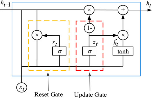
FIGURE 1. Structure of the GRU

In period t, the GRU receives input from two external sources, namely, the present state $x_t^{\prime }$ and the concealed state $h_{t-1}$. The operational workflow of the GRU can be segregated into two distinct steps.

4.1.3.1 Reset gate

This gate function reduces the risk of gradient explosion in the model by dropping some information about the data that is not relevant to the prediction moment and deciding how much information needs to be saved.

$r_t=\sigma \left(W_r\left[h_{t-1},x_t^{\prime }\right]\right).(30)$

4.1.3.2 Update gate

The reset gate has the same structure as the t update gate and determines the degree to which the low-weight information is forgotten and how much memory is retained to update to the current cell.

$u_t=\sigma \left(W_u\left[h_{t-1},x_t^{\prime }\right]\right).(31)$

The newly updated memory content utilizes the reset gate to preserve information related to the past and calculate the Hadamard product ($*$) of the reset gate r_t and $\left[h_{t-1},x_t^{\prime }\right]$. The Hadamard results will be summed and passed to the hyperbolic tangent activation function (tanh). Thence, h_t retains the influence of historical data on the current prediction and regulates the influx of input data by employing gating mechanisms, deciding what information should be propagated to the subsequent unit, avoiding the gradient disappearance problem.

$\left\{\begin{array}{l}{\widehat{h}}_t=\tanh \left(W_{\widehat{h}}\cdot \left[r_t\ast \left(h_{t-1},x_t\right)\right]\right)\\ h_t=\left(1-u_t\right)\ast h_{t-1}+u_t\ast {\widehat{h}}_t\end{array}\right..(32)$

4.1.4 ATT-CNN-GRU

The ATT-CNN is employed to find time series data patterns, which are imported as a whole into the GRU model for long time series prediction to improve prediction stability, and the steps are given as follows.

1. Data pre-processing: The data are normalized and then split into next sets according to the GRU model training method (Sutskever et al., 2013).

2. ATT-CNN unit: The pre-processed data are distinguished from their strong and weak features. The weak features are removed, and the strong features are extracted as the next unit input.

3. GRU unit: Utilizing the output from the preceding unit as input to construct the time series prediction model.

4. Output: Exporting the results of ATT-CNN-GRU prediction.

More training details can be found in the work of Vinvals et al. (2015), where the ATT-CNN-GRU is used to fast predict the state vector. Next, an OPTICS-based abnormal detection method is first introduced and combined with the ATT-CNN-GRU to handle the outliers.

4.2 Abnormal data detection and replacement

After obtaining the predicted state value, the corresponding measurement data can be obtained through the power flow equation (PF) (Tinney et al., 1967).

$\left\{\begin{array}{l}{P}_t^n=V_t^n{\displaystyle \sum _{n=1}^N}{V}_t^m\left(G^{nm}\cos {\theta }_t^{nm}+B^{nm}\sin {\theta }_t^{nm}\right)\\ Q_t^n=V_t^n{\displaystyle \sum _{n=1}^N}{V}_t^m\left(G^{nm}\sin {\theta }_t^{nm}-B^{nm}\sin {\theta }_t^{nm}\right)\\ P_t^{nm}=V_t^{n,2}{G}^{nm}-V_t^n{V}_t^m{G}^{nm}\cos {\theta }_t^{nm}-V_t^n{V}_t^m{G}^{nm}\sin {\theta }_t^{nm}\\ Q_t^{nm}=-V_t^{n,2}{B}^{nm}-V_t^n{V}_t^m{B}^{nm}\sin {\theta }_t^{nm}+V_t^n{V}_t^m{B}^{nm}\cos {\theta }_t^{nm}\end{array}\right..(33)$

For outliers such as missing and error measurements, the anomaly detection method is applied to deal with these outliers.

OPTICS is a commonly used detection algorithm, which can efficiency discover the oddly shape cluster. OPTICS creates a neighborhood $N_{\epsilon }\left(z_i^{*}\right)$ of radius ε for each $z_i^{*}$, and there should be no less than MinPts data points in the neighborhood, where $z_i^{*}$ is the new input measurement at time i. Some definitions are given as follows.

Directly density-reachable: If the new measurements $z_i^{*}$ and $z_j^{*}$ satisfy $z_i^{*}\in N_{\epsilon }\left(z_j^{*}\right)$ and $card\left(N_{\epsilon }\left(z_j^{*}\right)\right)\ge MinPts$, then $z_i^{*}$ is considered to be reachable by $z_j^{*}$ density directly, and $z_j^{*}$ is regarded as core object, where the $card\left(N_{\epsilon }\left(z_j^{*}\right)\right)$ denotes the quantity of elements contained in the set $N_{\epsilon }\left(z_j^{*}\right)$.

Density-reachable: For the dataset $z_r^{*},z_{r+1}^{*},\cdots ,z_{r+s}^{*}$, if $z_i^{*}i\in \left[r,r+s-1\right]$ can be reachable by $z_{i+1}^{*}$ density directly, then $z_i^{*}$ is density-reachable from $z_{i+1}^{*}$.

Density-connected: If $z_i^{*}$ and $z_j^{*}$ are reachable by $z_k^{*}$ density directly, then $z_i^{*}$ and $z_j^{*}$ are density-connected.

Core distance: The minimum neighborhood radius that makes $z_i^{*}$ a core object can be expressed as follows:

$cd\left(z\right)=\left\{\begin{array}{cc}d\left(z,N_{\epsilon }^a\left(z\right)\right),& \text{if}\left|N_{\epsilon }\left(z\right)\right|\ge MinPts\\ undefined,& \text{if\hspace{1em}}\left|N_{\epsilon }\left(z\right)\right|<MinPts\end{array}\right.,(34)$

where $N_{\epsilon }^a\left(z\right)$ denotes the data $N_{\epsilon }\left(z\right)$ that is the ath nearest neighbor to the data z, and z is the core object.

4.2.1 Reachability distance

The reachability distance is given as follows:

$rd\left(z_i^{*},z_j^{*}\right)=\left\{\begin{array}{cc}undefined& \text{if\hspace{1em}}card\left(N_{\epsilon }\left(z_i^{*}\right)\right)\le MinPts\\ \left.\max \left(cd\left(z_j^{*}\right),d\left(z_i^{*},z_j^{*}\right)\right)\right|& \text{if\hspace{1em}}card\left(N_{\epsilon }\left(z_i^{*}\right)\right)\ge MinPts\end{array}\right.,(35)$

where $rd\left(z_i^{*},z_j^{*}\right)$ is the minimum distance at which $z_i^{*}$ can be reachable by $z_j^{*}$ density directly, and $z_j^{*}$ is a core object.

In practical applications, the dispatch center only needs to import historical data into our KRR-UKF method and perform modeling and then collect real-time data to perform real-time filtering. Meanwhile, the model can also expand the training set based on the actual production data to optimize the filter. The specific flow of the robust KRR-UKF at time t is shown in Figure 2.

FIGURE 2

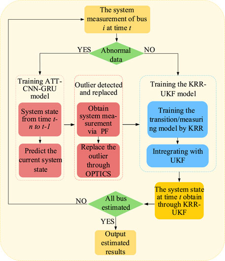
FIGURE 2. Flow chart of the robust KRR-UKF method.

The selection of parameters ε and MinPts can be found in the work of Ankerst et al. (1999). The OPTICS and ATT-CNN-GRU are used to handle the outliers, which consist of the following steps.

1. Computing reachability distance: Data z_i in new measurement dataset Z are selected randomly as the current object, and then, the reachability distance of all other measurements in Z is calculated with respect to the current object.

2. Marking the data: Data with the smallest reachability distance from the current object are found, and then, the current object is replaced with that set of data and is marked as processed.

3. Getting the smallest reachability distance: The reachable distances of the unprocessed data from the current object are calculated in turn, and if any of these reachable distances is smaller than the reachable distance calculated in step 2, then the corresponding data are replaced with the current object. If not, the current object remains unchanged.

4. Iteration: Steps 2 and 3 are repeated until all data in Z have been processed.

5. Classifying the data: The calculated reachable distance ${\epsilon }^{\prime }$ of each data is compared with $\epsilon$; if ${\epsilon }^{\prime }$ < $\epsilon$, then the reachable distance is meaningful, and the corresponding data are considered normal. Otherwise, it is marked as outlier.

6. Predicting the state: The predicted measurements in period t of node n can be computed via the ATT-CNN-GRU.

${\widehat{z}}^n=\left\{{\widehat{P}}_t^n,{\widehat{Q}}_t^n,{\widehat{P}}_t^{nm},{\widehat{Q}}_t^{nm}\right\}.(36)$

7. Outlier replacement: If the input data are marked as outliers, the corresponding measurements are replaced by (39).

5 Case studies

Simulations are carried on a IEEE 33-bus system and a realistic 109-bus system from a city in China to verify the robustness under different circumstances. The ATT-CNN-GRU and KRR-UKF models are developed using PYTHON on the NVIDIA GTX-1660TI with 16 GB RAM. The system state and measurement dataset are obtained from the MATPOWER toolkit. We use the mean absolute error (MAE) and root mean squared error (RMSE) (Hossain et al., 2020).

5.1 IEEE 33-bus system

The load data on Belgian grid of 2020 are selected to generate 8,760 measurement state sets, in which a total of 4,000 sets of data are randomly selected as the training set. The load data of 2021 on Belgian grid are used to generate 8,760 data as the test set.

5.2 Scenario 1: with only Gaussian noise

We assume that the noise follows the Gaussian distribution. We compare the UKF with the KRR-UKF and GP-FSE (Ji et al., 2021) under ideal conditions. It is noted that in the existing references on PSSE based on Kalman filtering, in this section, Gaussian noise with a mean value of 0 and a variance of 10⁻⁶ is added into the sample data, and the filter performance of the three algorithms is shown in Figure 3.

FIGURE 3

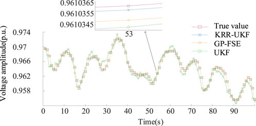
FIGURE 3. Filtering result of node 6 of three algorithms.

As shown in Figure 3, under the ideal conditions, there is a substantial disparity between the estimated state obtained through UKF and the true value. Furthermore, we can see from Figure 3, as data-driven algorithms, the KRR-UKF and GP-FSE have a better prediction performance than the UKF, and the difference between the estimated state via the KRR-UKF and the actual value is exceedingly minute. This is because kernel ridge regression is a powerful non-parametric tool that has the capability to acquire noise characteristics and smoothing parameters from the training data; thus, it is also deduced that the accuracy of GP-FSE is slightly inferior to the method we have introduced.

To intuitively demonstrate the effectiveness of these filters, the MAE and RMSE of the KRR-UKF are shown in Figure 4A. In addition, to further illustrate the robustness of our methods, Gaussian noise characterized by a mean of 0 and a variance of and 10⁻⁴ is added to the sample data.

FIGURE 4

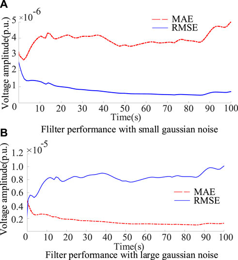
FIGURE 4. KRR-UKF performance on node 6. (A) MAE and RMSE of the KRR-UKF with small Gaussian of noise (B) MAE and RMSE of the KRR-UKF with large Gaussian of noise.

Figure 4 illustrated the MAE and RMSE of the KRR-UKF algorithm maintained at the range of 10⁻⁵–10⁻⁶ under different noises. The proposed KRR maps the non-linear correlation into high dimension for precisely tracking data characteristics. Then, the five-fold cross-validation method also assigns more appropriate parameters to the noise data for optimizing the estimated results. As displayed in Figure 4A, the data-driven approach we propose exhibits remarkable accuracy and stability, and Figure 4B shows that the proposed method still has excellent prediction accuracy when the noise covariance is increased to 10⁻⁴. Furthermore, the RMSE is more sensitive to predicting abnormal values, but the RMSE of the KRR-UKF estimation results remains at 10⁻⁶ under different noise levels, which demonstrates that the method has good robustness to the Gaussian noise.

5.3 Scenario 2: with non-Gaussian noise

To test KRR-UKF performances under different non-Gaussian noises, the weights are 0.95 and 0.05, the bimodal Gaussian noise with covariance matrices of 10⁻⁶ I and 10⁻⁵ I is added. The KRR-UKF has the ability to assign higher weight to the predicted value information with small deviation, thus filtering out non-Gaussian noise data.

In Figure 5 (a), when the degree of noise deviating from the Gaussian distribution increases, the proposed KRR-UKF still maintains the estimation performance similar to scenario 1, and its MAE and RMSE can be kept at 10⁻⁶ and 10⁻⁵, respectively, which proves that the method can filter non-Gaussian noises. In order to showcase the robustness of the KRR-UKF approach, Laplace noise and Cauchy noise are added, the covariance matrix of Laplace is 10⁻⁵ I, and the location parameter and scale location parameter are 0 and 10⁻⁵I, respectively.

FIGURE 5

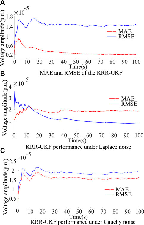
FIGURE 5. Filtering performance of node 6 in non-Gaussian of noise. (A) In small noise, (B) under Laplace noise, and (C) under Cauchy noise.

In Figure 5, the MAE of the KRR-UKF filter increases slightly, and the error remains at 10⁻⁵, which indicates that the proposed KRR-UKF is robust to different non-Gaussian noises. To fully verify the robustness of the KRR-UKF, noises that further deviate from the Gaussian distribution are added to the datasets of the KRR-UKF and GP-FSE, the bimodal Gaussian noise covariance matrices of the two models are 10⁻⁶ I and 10⁻⁴ I, respectively; and the noise weight ratio is gradually changed from 0.95/0.05 to 0.5/0.5, with a step size of 0.05.

In Table 1, both methods show an increase in MAE as the deviation of non-Gaussian noise grows and finally remains at the order of 10⁻⁴, but due to the lack of correction of predict equation, the MAE of GP-FSE has nearly tripled, and its RMSE increases to 1.190 × 10⁻⁴, which means the instability of GP-FSE increases further. However, the kernel ridge regression method can optimize the parameters; thus, enabling the model adapts the unknown noise exactly and corrects the estimation results more accurately. The RMSE of the proposed method fluctuates between 5.857 × 10⁻⁵ and 1.231 × 10⁻⁵, which demonstrates that the proposed KRR-UKF has good robustness and stronger stability.

TABLE 1

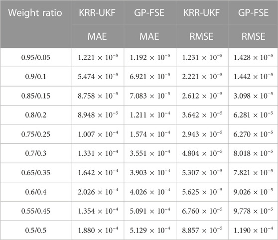
TABLE 1. Performance of the two algorithms under different weight noises.

5.4 Scenario 3: with reduced measurement redundancy

The proposed KRR-UKF method uses the historical data to model the measuring equation in certain topology network; the ratio between the number of measurement quantities and state quantities is defined as measurement redundancy, which is crucial to determine the result of state estimation. The historical data used in this model include nodal voltage, phase angle (V, θ), nodal active and reactive power (P, Q), and associated branch (P^nm, Q^nm). We take the voltage of bus 18 as the test state consistent with scenario 2. The 100s estimated results are compared with the calculated value using PF under noiseless condition.

In Table 2, as the measurement redundancy increases, the MAE and RMSE gradually decline, which is due to the facts that more measurement information can be used to eliminate the influence of bad data and errors. The parallel computing method can compute the state mapped values of multiple measurements simultaneously, so when the redundancy increases, there is no significant increase in consumption time. When the redundancy reaches 4, the time consumption of the KRR-UKF only increased 33% and remained in the order of milliseconds, indicating that the proposed method can work properly with reduced measurement redundancy.

TABLE 2

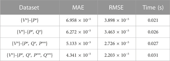
TABLE 2. Performances of the KRR-UKF using different datasets.

5.5 Scenario 4: under network reconfiguration

To demonstrate the proposed filter performances when the topology network changes, we take node 24 as an example. Table 3 gives two network structures, and the topology changes from structure A to structure B at 50s. Half of the KRR-UKF training set comes from structure A and half from topology B.

TABLE 3

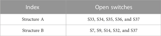
TABLE 3. Two different structures of the IEEE-33 system.

The performance under the condition of small Gaussian noise is plotted in Figure 6.

FIGURE 6

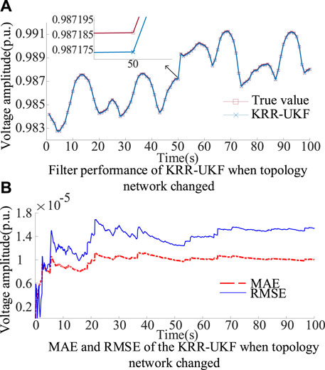
FIGURE 6. Filtering performance of node 24 when topology changes. (A) Filter performance of the KRR-UKF when the topology network changed. (B) MAE and RMSE of the KRR-UKF when the topology network changed.

In Figure 6, the voltage amplitude estimated by the KRR-UKF aligns closely with the actual value. It should be noted that the proposed KRR-UKF can model only based on the input data, free from the limitations of the mechanism model. Thus, when the topology network changes at 50s, both RMSE and MAE can be maintained at around 10⁻⁵. It can be inferred that the approach is capable of performing under network reconfiguration by simply expanding the training set, which is sufficient to deal with the topological changes in the distribution network.

5.6 Scenario 5: with abnormal or missing data

Due to communication channel interruption, flicker, and abnormal data transmission problems in the data acquisition system, abnormal or missing data may occur. To demonstrate the feasibility of using the ATT-CNN-GRU for outlier replacement, this section takes the voltage of node 11 as an example. This paper sets up two cases.

Case 1. assumed that 30% of the active power is abnormal in the measurement data of node 11, and the gross error is 15%.

Case 2. assumed that there are 20% missing in the measurement data of node 11.

The OPTICS clustering algorithm is applied to detect and label outliers, and then, the proposed ATT-CNN-GRU is used to predict and replace the abnormal measurements. The model tuning mainly includes the number of convolutional layers, and the voltage estimation results of different layers are shown in Table 4.

In Table 1, the estimation accuracy and estimation efficiency of the CNN are optimal for a number of layers of 2. We list the voltage prediction results of ATT-CNN-LSTM and the ATT-CNN-GRU with the same structure in Table 5 to substantiate the effectiveness. Comparing with ATT-CNN-LSTM, the prediction accuracy and stability of the ATT-CNN-GRU improved by 12.51% and 16.39%, respectively, because our method optimizes parameter structure and integrates global and local features to avoid losing necessary feature data. Thence, the time required to predict the data reduces consumption of time by 14.75% compared with ATT-CNN-LSTM, which proves that the method can accurately and efficiently replace the bad data. Therefore, the ATT-CNN-GRU is selected to handle outliers, and the filtering results of the KRR-UKF after ATT-CNN-GRU replacing the anomalous data are shown in Figure 7.

In Figure 7A, the MAE of the KRR-UKF maintained at 10⁻⁵, through the ATT-CNN module, the improved GRU can extract coarse-grained features from the fine-grained features in data. To a certain extent, it can solve the problems of memory loss and gradient dispersion induced by excessively long steps in the GRU, which provides the proposed method with accurate measurement data for filtering. From the results of Figure 7 (b), the filtering curve fluctuates very slightly and ensures filtering accuracy.

In Table 6, the WLS has the least calculation time, but the estimation accuracy is the worst. Nevertheless, the KRR-UKF uses improved LSTM algorithms for data replacement, so there will be time loss when abnormal conditions occur, and still has milli-second calculation time, which fulfills the criteria for achieving real-time state estimation accuracy.

The KRR-UKF also displays relatively heightened estimation accuracy under abnormal conditions with an RMSE of 3.4 × 10⁻⁵, which is nearly 33% accurate than a GP-FSE. Hence, the KRR-UKF emerges as a relatively optimal choice for real-time state estimation in the IEEE 33-bus system.

TABLE 4

TABLE 4. Estimation results for different numbers of convolutional layers.

TABLE 5

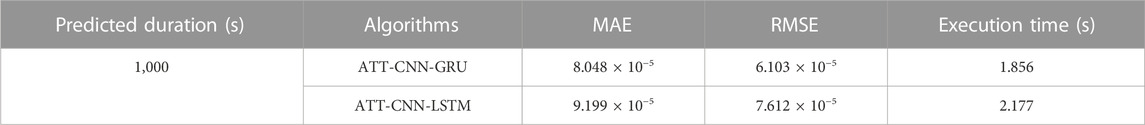
TABLE 5. Comparison of forecast results of different algorithms.

FIGURE 7

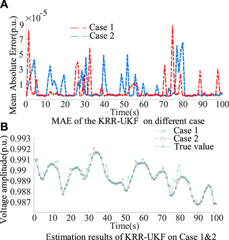
FIGURE 7. Filtering performance for node 11. (A) MAE of the KRR-UKF in case 1&2. (B) estimation results of KRR-UKF in case 1&2.

TABLE 6

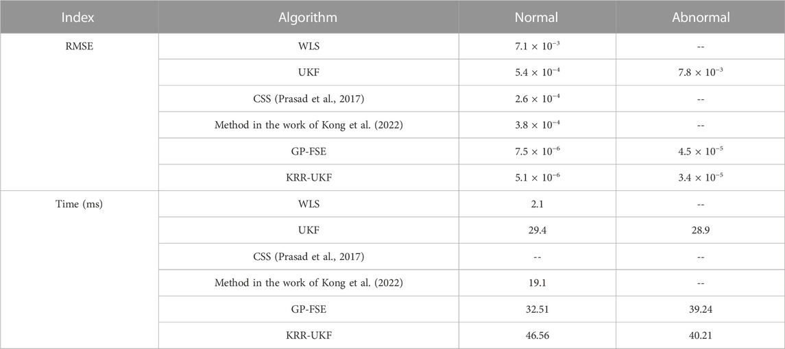
TABLE 6. RMSE and computing time of different algorithms.

5.7 109-bus system from a city in China

In this section, a 109-bus distribution network system from a city in China is selected for a practical application test. We obtained the operation data in August 2020, randomly selected 2,880 groups as the training set, and used 2,880 groups of data in August 2021 as the testing dataset. We randomly choose 20% data from the test set for exception handling, in which 10% data are replaced by 0 value and 10% data are randomly reduced by 15%. The estimation results of the KRR-UKF, GP-FSE, and UKF under normal conditions are shown in Figure 8.

FIGURE 8

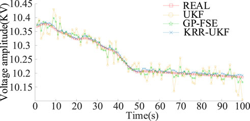
FIGURE 8. Filtering performance of different algorithms.

As shown in Figure 8, the filtering curves UKF fluctuate, and the accuracy decreases due to unknown noise, which is affected by unknown noise and has many deviation points. However, the KRR-UKF can maintain the same trend as the true value in general.

In Table 7, comparing with the simulation result in scenario 1, the accuracy of the UKF is greatly reduced due to the unknown noise. The GP-FSE model is affected by non-Gaussian noise in training data and lack of predictive steps to correct it. The error increases to 10⁻³. However, the KRR-UKF still shows favorable performance, whose RMSE is 3.22 × 10⁻⁴. The calculation time of the KRR-UKF is 0.292 s, which also fulfills the requirements of real time state estimation. In conclusion, the proposed KRR-UKF has sufficient accuracy and robustness that can be applied in practical engineering.

TABLE 7

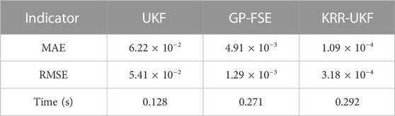
TABLE 7. Comparison of different filters.

6 Conclusion

In this paper, a KRR-UKF method, which can improve the exactitude and robustness of state estimation, is proposed. The test results prove that the proposed KRR-UKF method can filter unknown noise in the power system, and the ATT-CNN-GRU can enhance the accuracy of the predicting outlier, as well as in the conditions of topology network changes or reduced measurement redundancy. Furthermore, the performances of the KRR-UKF method are only related to the dataset; that is to say, there is no need to consider the actual physical model. Moreover, compared to existing algorithms, the KRR-UKF exhibits significant enhancements in both estimation accuracy and computational efficiency.

Although the KRR-UKF shows extraordinary performances on state estimation, when the system is in three-phase unbalanced states, the results of state estimation may become worse. Furthermore, the method introduced in this paper necessitates a considerable volume of historical operational data for model training, imposing a slightly higher requirement on data accuracy without considering the placement of measurement equipment and acquisition accuracy in real industry. Further verification of the feasibility of application to industry is still required.

Data availability statement

The data analyzed in this study are subject to licenses/restrictions: The source of the dataset is the project provider, which is not convenient to disclose. Requests to access these datasets should be directed to SZ, zsmphys@sdust.edu.cn.

Author contributions

WZ: data curation, supervision, and writing–original draft. SZ: conceptualization, methodology, resources, and writing–review and editing. YZ: investigation and writing–original draft. GX: formal analysis and writing–original draft. HM: validation and Writing–original draft.

Conflict of interest

WZ and GX were employed by Zhuhai XJ Electric Co., Ltd.

The remaining authors declare that the research was conducted in the absence of any commercial or financial relationships that could be construed as a potential conflict of interest.

Publisher’s note

All claims expressed in this article are solely those of the authors and do not necessarily represent those of their affiliated organizations, or those of the publisher, the editors, and the reviewers. Any product that may be evaluated in this article, or claim that may be made by its manufacturer, is not guaranteed or endorsed by the publisher.

References

Ankerst, M., Breunig, M. M., Kriegel, H. P., and Sander, J. (1999). OPTICS: ordering points to identify the clustering structure. ACM Sigmod Rec. 28 (2), 49–60. doi:10.1145/304181.304187

CrossRef Full Text | Google Scholar

Arlot, S., and Celisse, A. (2010). A survey of cross-validation procedures for model selection. Stat. Surv. 4. doi:10.1214/09-ss054

CrossRef Full Text | Google Scholar

Bai, X., Qu, L., and Qiao, W. (2016). Robust AC optimal power flow for power networks with wind power generation. IEEE Trans. Power Syst. 31, 4163–4164. doi:10.1109/tpwrs.2015.2493778

CrossRef Full Text | Google Scholar

Dang, L., Chen, B., Ma, W., and Ren, P., (2020). Robust power system state estimation with minimum error entropy unscented Kalman filter. IEEE Trans. Instrum. Meas. 69, 8797–8808. doi:10.1109/tim.2020.2999757

CrossRef Full Text | Google Scholar

Du, Q., Bo, Z., Dong, Y., and Luo, X. S. (2010). Effect of noise on erosion of safe basin in power system. Nonlinear Dyn. 61, 477–482. doi:10.1007/s11071-010-9663-0

CrossRef Full Text | Google Scholar

Ghahremani, E., and Kamwa, I. (2016). Local and wide-area PMU-based decentralized dynamic state estimation in multi-machine power systems. IEEE Trans. Power Syst. 31, 547–562. doi:10.1109/tpwrs.2015.2400633

CrossRef Full Text | Google Scholar

Guo, L., Liu, W., Li, X., Liu, Y., Jiao, B., Wang, W., et al. (2014). Energy management system for stand-alone wind-powered-desalination microgrid. IEEE Trans. Smart Grid 7 (2), 1–1087. doi:10.1109/tsg.2014.2377374

CrossRef Full Text | Google Scholar

Hara, K., Saito, D., and Shouno, H. (2015). “Analysis of function of rectified linear unit used in deep learning,” in International Joint Conference on Neural Networks 2015, Killarney, Ireland, July 12–16, 2015, 1–8.

CrossRef Full Text | Google Scholar

Hochreiter, S., and Schmidhuber, J. (1997). Long short-term memory. Neural Comput. 9 (8), 1735–1780. doi:10.1162/neco.1997.9.8.1735

PubMed Abstract | CrossRef Full Text | Google Scholar

Hoerl, A. E., and Kennard, R. W. (1970). Ridge regression: biased estimation for nonorthogonal problems. Technometrics 12 (1), 55–67. doi:10.1080/00401706.1970.10488634

CrossRef Full Text | Google Scholar

Hossain, M., and Mahmood, H. (2020). Short-term photovoltaic power forecasting using an LSTM neural network and synthetic weather forecast. IEEE Access 8, 172524–172533. doi:10.1109/access.2020.3024901

CrossRef Full Text | Google Scholar

Jensen, S. K., Pedersen, T. B., and Thomsen, C. (2017). Time series management systems: a survey. IEEE Trans. Knowl. Data Eng. 29, 2581–2600. doi:10.1109/tkde.2017.2740932

CrossRef Full Text | Google Scholar

Ji, X., Yin, Z., Zhang, Y., Wang, M., Zhang, X., Zhang, C., et al. (2021). Real-time robust forecasting-aided state estimation of power system based on data-driven models. Int. J. Electr. Power and Energy Syst. 125, 106412. doi:10.1016/j.ijepes.2020.106412

CrossRef Full Text | Google Scholar

Julier, S., Uhlmann, J., and Durrant-Whyte, H. F. (2000). A new method for the nonlinear transformation of means and covariances in filters and estimators. IEEE Trans. Automatic Control 45 (3), 477–482. doi:10.1109/9.847726

CrossRef Full Text | Google Scholar

Kalman, R. E. (1960). A new approach to linear filtering and prediction problems.

Google Scholar

Ko, J., Klein, D. J., and Fox, D. (2007). “Gaussian processes and reinforcement learning for identification and control of an autonomous blimp,” in Proceedings 2007 IEEE International Conference on Robotics and Automation, Roma, Italy, 14 April 2007, 742–747.

CrossRef Full Text | Google Scholar

Kollias, D., and Zafeiriou, S. (2021). Exploiting Multi-CNN features in CNN-RNN based dimensional emotion recognition on the OMG in-the-Wild dataset. IEEE Trans. Affect. Comput. 12 (12), 595–606. doi:10.1109/taffc.2020.3014171

CrossRef Full Text | Google Scholar

Kong, X., Zhang, X., Zhang, X., Wang, C., Chiang, H. D., and Li, P. (2022). Adaptive dynamic state estimation of distribution network based on interacting multiple model. IEEE Trans. Sustain. Energy 13 (2), 643–652. doi:10.1109/tste.2021.3118030

CrossRef Full Text | Google Scholar

Mestav, K. R., Luengo-Rozas, J., and Tong, L. (2018). “State estimation for unobservable distribution systems via deep neural networks,” in 2018 IEEE Power and energy Society General Meeting (PESGM), Portland, Oregon, 5-10 August 2018, 1–5.

CrossRef Full Text | Google Scholar

Mestav, K. R., Luengo-Rozas, J., and Tong, L. (2019b). Bayesian state estimation for unobservable distribution systems via deep learning. IEEE Trans. Power Syst. 34, 4910–4920. doi:10.1109/tpwrs.2019.2919157

CrossRef Full Text | Google Scholar

Mestav, K. R., and Tong, L. (2019a). “State estimation in smart distribution systems with deep generative adversary networks,” in 2019 IEEE International Conference on Communications, Control, and Computing Technologies for Smart Grids, Beijing, China, October 2019, 1–6.

CrossRef Full Text | Google Scholar

Murphy, K. P. (2012). Machine learning: a probabilistic perspective. Massachusetts, United States: Mit Press.

Google Scholar

Netto, M., and Mili, L. (2018). A robust data-driven Koopman Kalman filter for power systems dynamic state estimation. IEEE Trans. Power Syst. 33, 7228–7237. doi:10.1109/tpwrs.2018.2846744

CrossRef Full Text | Google Scholar

Prasad, S., and Vinod Kumar, D. M. (2017). Hybrid fuzzy charged system search algorithm-based state estimation in distribution networks. Eng. Sci. Technol. 20 (3), 922–933. doi:10.1016/j.jestch.2017.04.002

CrossRef Full Text | Google Scholar

Rosenthal, W. S., Tartakovsky, A. M., and Huang, Z. (2017). Ensemble kalman filter for dynamic state estimation of power grids stochastically driven by time-correlated mechanical input power. IEEE Trans. Power Syst. 33 (4), 3701–3710. doi:10.1109/tpwrs.2017.2764492

CrossRef Full Text | Google Scholar

Samuelsson, O., Hemmingsson, M., Nielsen, A. H., Pedersen, K., and Rasmussen, J. (2006). Monitoring of power system events at transmission and distribution level. IEEE Trans. Power Syst. 21, 1007–1008. doi:10.1109/tpwrs.2006.873014

CrossRef Full Text | Google Scholar

Sutskever, I. (2013). Training recurrent neural networks. Toronto on Canada: University of Toronto.

Google Scholar

Tahmasebi, P., and Hezarkhani, (2011). Application of a modular feedforward neural network for grade estimation. Nat. Resour. Res. 20, 25–32. doi:10.1007/s11053-011-9135-3

CrossRef Full Text | Google Scholar

Tinney, W. F., and Hart, C. E. (1967). Power flow solution by Newton's method. IEEE Trans. Power Apparatus Syst., 1449–1460. PAS-86. doi:10.1109/tpas.1967.291823

CrossRef Full Text | Google Scholar

Vinyals, O., Toshev, A., and Bengio, S. (2015). “Show and tell: a neural image caption generator,” in Proceedings of the IEEE Conference on Computer Vision and Pattern Recognition. 2015, Boston, Massachusetts, 7-12 June 2015, 3156–3164.

CrossRef Full Text | Google Scholar

Weng, Y., Negi, R., Faloutsos, C., and Ilic, M. D. (2016). Robust data-driven state estimation for smart grid. IEEE Trans. Smart Grid 8 (4), 1956–1967. doi:10.1109/tsg.2015.2512925

CrossRef Full Text | Google Scholar

Wu, H., Xu, Z., and Wang, M. (2022). Unrolled spatiotemporal graph convolutional network for distribution system state estimation and forecasting[J]. IEEE Trans. Sustain. Energy 14 (1), 297–308. doi:10.1109/TSTE.2022.3211706

CrossRef Full Text | Google Scholar

Zadeh, R. A., Ghosh, A., and Ledwich, G. (2010). Combination of Kalman filter and least-error square techniques in power system. IEEE Trans. Power Deliv. 25, 2868–2880. doi:10.1109/tpwrd.2010.2049276

CrossRef Full Text | Google Scholar

Zhang, H., Yu, T., Wang, W., Jiao, W., Chen, W., Zhong, Q., et al. (2020). Characterization of volatile profiles and marker substances by HS-spme/GC-MS during the concentration of coconut jam. Deep Reinf. Learn. 9, 347–364. doi:10.3390/foods9030347

PubMed Abstract | CrossRef Full Text | Google Scholar

Zhang, L., Wang, G., and Giannakis, G. B. (2019). Real-time power system state estimation and forecasting via deep unrolled neural networks. IEEE Trans. Signal Process. 67 (15), 4069–4077. doi:10.1109/tsp.2019.2926023

CrossRef Full Text | Google Scholar

Zhao, J. (2018). Dynamic state estimation with model uncertainties using $H_\infty$ extended kalman filter. IEEE Trans. Power Syst. 33, 1099–1100. doi:10.1109/tpwrs.2017.2688131

CrossRef Full Text | Google Scholar

Zhao, J., and Mili, L. (2018). A robust generalized-maximum likelihood unscented Kalman filter for power system dynamic state estimation. IEEE J. Sel. Top. Signal Process. 12, 578–592. doi:10.1109/jstsp.2018.2827261

CrossRef Full Text | Google Scholar

Zhao, J., Mili, L., and Gomez-Exposito, (2019b). Constrained robust unscented kalman filter for generalized dynamic state estimation. IEEE Trans. Power Syst. 34, 3637–3646. doi:10.1109/tpwrs.2019.2909000

CrossRef Full Text | Google Scholar

Zhao, J., Qi, J., Huang, Z., Meliopoulos, A. P. S., Gomez-Exposito, A., Netto, M., et al. (2019a). Power system dynamic state estimation: motivations, definitions, methodologies, and future Work. IEEE Trans. Power Syst. 34, 3188–3198. doi:10.1109/tpwrs.2019.2894769

CrossRef Full Text | Google Scholar

Nomenclature