Optimal site and size of FACTS devices with the integration of uncertain wind generation on a solution of stochastic multi-objective optimal power flow problem

To reduce the Carbon footprint and reduce emissions from the globe, the world has kicked-off to leave reliance of fossil fuels and generate electrical energy from renewable energy sources. The MOOPF problem is becoming more complex, and the number of decision variables is increasing, with the introduction of power electronics-based Flexible AC Transmission Systems (FACTS) devices. These power system components can all be used to increase controllability, effectiveness, stability, and sustainability. The added uncertainty and variability that FACTS devices and wind generation provide to the power system makes it challenging to find the right solution to MOOPF issues. In order to determine the best combination of control and state variables for the MOOPF problem, this paper develops three cases of competing objective functions. These cases include minimizing the total cost of power produced as well as over- and underestimating the cost of wind generation, emission rate, and the cost of power loss caused by transmission lines. In the case studies, power system optimization is done while dealing with both fixed and variable load scenarios. The proposed algorithm was tested on three different cases with different objective functions. The algorithm achieved an expected cost of $833.014/h and an emission rate of conventional thermal generators of 0.665 t/h in the case 1. In Case 2, the algorithm obtained a minimum cost of $731.419/h for active power generation and a cost of power loss is 124.498 $/h for energy loss. In Case 3, three objective functions were minimized simultaneously, leading to costs of $806.6/h for emissions, 0.647 t/h, and $214.9/h for power loss.

1 Introduction

Deregulation of power systems aims to introduce competition and promote efficiency in the market. This has resulted in the unbundling of vertically integrated utilities into separate entities responsible for the generation, transmission, and distribution of power. In deregulated power systems, the government has opened up the power market to competition and private investment. This means that private companies are allowed to own and operate power plants, transmission lines, and distribution systems, and sell electricity to consumers at market prices. The market determines the price of electricity, but the government still regulates the quality and dependability of service and may set criteria for renewable energy and emissions. Therefore, modern developments such as the integration of Renewable Energy, aging infrastructure, large demand variability, grid modernization, and environmental concerns pose a number of issues for the power system (Duman et al., 2020). Overall, ensuring the stability, resiliency, and sustainability of the electricity system necessitates a combination of cutting-edge technology, policies, and laws to meet these challenges head-on. The generation, transmission, and distribution of electricity are all undergoing changes as a result of these current power system developments. While they present potential to improve power system efficiency, dependability, and sustainability, they also present obstacles that must be overcome to guarantee the secure and reliable operation of the grid (Wei et al., 2004). The power system has benefited greatly from the incorporation of sophisticated generation technologies like wind and solar, which have reduced carbon emissions and increased the usage of renewable energy sources. Intermittency, Grid Integration, Power Quality, and Forecasting are just a few of the difficulties that it has posed for power system management and planning (Abdo et al., 2018). In order to boost the power system’s efficiency, dependability, and performance, FACTS devices can be used (Ongsakul and Bhasaputra, 2002). Installation in both new and existing power systems makes them useful for a wide variety of voltage regulation and renewable energy integration tasks. FACTS devices play a crucial role in helping to keep the voltage profile of the power system stable (Chen et al., 2018a). While the intermittent nature of renewable energy sources like wind and solar can lead to voltage fluctuations that disrupt the operation of other devices in the system (Zhang et al., 2016), FACTS devices can swiftly and correctly adjust voltage levels, preventing damage to the system. FACTS devices can improve power transmission efficiency in addition to supporting a wider range of voltages. It is not always possible to place wind and solar generators close to load centers, which might increase transmission losses and limit the amount of power that can be transferred (Warid et al., 2016). By regulating the flow of reactive power and decreasing transmission losses, FACTS devices like static var compensators (SVCs) and thyristor-controlled series capacitors (TCSCs) can enhance power transfer capability. By providing voltage support, boosting power transfer capabilities, and minimizing power losses, FACTS devices can make up for the shortcomings of wind and solar integration. FACTS devices will become even more important in maintaining the power grid’s reliability, efficiency, and stability as renewable energy sources like wind and solar continue to play a larger role in the generation mix (Biswas et al., 2018). Therefore, it is crucial to do an OPF analysis that accounts for both renewable energy sources and FACTS technology (Varadarajan and Swarup, 2008; Kumar and Premalatha, 2015; Li et al., 2019).

Nonlinear programming approaches, such as the gradient-based quasi-newton method (Mahdad and Srairi, 2016), interior point methods (Abaci and Yamacli, 2016), and evolutionary algorithms (Ali et al., 2023a), can be used to solve the classic OPF issue. The best values for the controllable variables that simultaneously meet the operating constraints and lower the cost of power generation and distribution are found in order to solve the OPF problem. The solutions to the OPF problem can be used to help with power system planning decisions, such as selecting the best combination of generation technologies, expanding the transmission system, or putting demand-side management plans into action. Compared to conventional techniques like Bender decomposition, Interior Point approaches, and gradient-based, metaheuristic algorithms have a number of advantages. They are highly scalable, robust, capable of global optimization, easily parallelizable, and flexible to handle different problem formulations. These advantages make metaheuristic algorithms a popular choice for solving large-scale optimization problems in various domains.

In the recent few decades, metaheuristic algorithm attains the focus of researchers to solve complex OPF problems because of providing a powerful and flexible tool and can help researchers and practitioners find better solutions to complex power system optimization challenges especially those involving multiple objectives and constraints. For the solution of single objective OPF these include; genetic algorithm (GA) (Kumari and Maheswarapu, 2010), evolutionary programming (EP) (Wei et al., 2004), developed Gray wolf optimization (DGWO) (Abdo et al., 2018); tabu search (TS) (Ongsakul and Bhasaputra, 2002), improved krill herd algorithm (IKHA) (Chen et al., 2018a); particle swarm optimization (PSO) (Zhang et al., 2016), Jaya algorithm (Warid et al., 2016), differential evolution (DE) (Varadarajan and Swarup, 2008; Biswas et al., 2018), modified coyote optimization algorithm (MCOA) (Li et al., 2019), adaptive real coded biogeography-based optimization (ARCBBO) (Kumar and Premalatha, 2015), adaptive partitioning flower pollination algorithm (APFPA) (Mahdad and Srairi, 2016), differential search algorithm (DSA) (Abaci and Yamacli, 2016), Improved artificial bee colony algorithm (IABC) (Ali et al., 2023a), moth swarm algorithm (MSA) (Mohamed et al., 2017), improved colliding bodies optimization algorithm (ICBO) (Bouchekara et al., 2016) and backtracking search optimization algorithm (BSA) (Chaib et al., 2016) have been employed for the solution to the single objective OPF problem. The main drawback of this research appears to be that it primarily concentrates on single or weighted sum multi-objective optimum power flow (MOOPF) problems. More investigation is required to create more precise and efficient algorithms that can tackle the issue under a variety of operating circumstances and uncertainties. When it comes to optimizing the operation of power systems, single-objective metaheuristics may not be the most suitable approach. This is due to the complexities of such a system, which require more advanced optimization techniques to effectively manage. Multi-objective evolutionary algorithms (MOEAs) can be better suited for this purpose. These algorithms can better handle the complexities of a power system making them more effective than single objective metaheuristics.

Several MOEAs have been applied to solve Multi-objective OPF (MOOPF) problem reviewed in (Niu et al., 2014; Skolfield and Escobedo, 2022) considering conventional thermal generators; these includes: enhanced GA (EGA) (Kumari and Maheswarapu, 2010), shuffle frog leaping algorithm (SFLA) (Niknam et al., 2011), quasi-oppositional teaching learning based optimization (QOTLBO) (Mandal and Kumar Roy, 2014), modified imperialist competitive algorithm (MICA) (Ghasemi et al., 2014), Multi-objective DE (MDE) (Shaheen et al., 2016), multi-objective modified ICA (MOMICA) (Ali et al., 2023b), modified TLBO (MTLBO) (Shabanpour-Haghighi et al., 2014), modified gaussian bare-bones ICA (MGBICA) (Ghasemi et al., 2015), non-dominated sorting gravitational search algorithm (NSGSA) (Bhowmik and Chakraborty, 2015), improved strength Pareto evolutionary algorithm 2 (I-SPEA2) (Yuan et al., 2017), multi-objective evolutionary algorithm based decomposition (MOEA-D) (Zhang et al., 2016), enhanced self-adaptive differential evolution (ESDE-MC) (Pulluri et al., 2017), novel quasi-oppositional modified Jaya algorithm (QOMJaya) (Ali et al., 2023c), multi-objective dimension-based firefly algorithm (MODFA) (Chen et al., 2018b), semidefinite programming (SDP) (Abbas et al., 2022), improved normalized normal constraint (INNC) (Rahmani and Amjady, 2018), multi-objective firefly algorithm with a constraints-prior pareto-domination (MOFA-CPD) (Chen et al., 2018c), novel hybrid bat algorithm with constrained pareto fuzzy dominant (NHBA-CPFD) (Habib et al., 2022), modified pigeon-inspired optimization algorithm (MIPO) (Chen et al., 2020), and interior search algorithm (ISA) (Chandrasekaran, 2020). In these papers, the integration of renewable energy sources was not considered. Moreover, the integration of wind and solar generation, which are increasingly important in modern power systems. Wind and solar power are clean, can significantly reduce greenhouse gas emissions, and are independent of fossil fuels. System operators can optimize power system management to make the most of renewable energy resources like wind and solar by including them into the MOOPF problem. The inclusion of renewable energy sources in the MOOPF problem also allows for the optimization of multiple objectives such as minimizing cost, reducing emissions, and ensuring system reliability, all of which are critical for the sustainable operation of power systems. Therefore, the integration of wind and solar power into the MOOPF problem is essential to ensure the optimal use of renewable energy resources and to meet the energy needs of society in a sustainable and reliable manner.

Several single objective EAs considering uncertainties in wind generation were implemented to solve the OPF problem that includes; self-adaptive evolutionary programming (SAEP) (Shi et al., 2012), Gbest-guided ABC (GABC) (Roy and Jadhav, 2015) modified bacteria foraging algorithm (MBFO) (Panda et al., 2014; Ali et al., 2023d). Whereas these papers did not employ MOEAs and do not consider the impacts of FACTS devices. Multi-objective optimal power flow (MO-OPF) is a complex optimization problem that seeks to simultaneously minimize multiple objectives such as generation cost, transmission losses, and environmental impact while satisfying various system constraints. FACTS devices can provide several specific advantages in MO-OPF problems, such as improving voltage stability, enhancing power transfer capability, reducing operating costs, better utilizing existing infrastructure, and offering flexibility and adaptability in optimizing power flow (Benabid et al., 2009; Sebaa et al., 2014; Ziaee and Choobineh, 2017a; Agrawal et al., 2018; Shafik et al., 2019).

The optimal power flow (OPF) problem has been the subject of numerous academic investigations, with many of them employing single-objective evolutionary algorithms (EAs) to find a solution. Hybrid tabu search and simulated annealing (TS-SA) (Ongsakul and Bhasaputra, 2002), DE (Basu, 2008), fuzzy-based improved comprehensive-learning particle swarm optimization (FBICLPSO) (Naderi et al., 2019), hybrid PSO-PS (Berrouk and Bounaya, 2018), Chaotic krill herd algorithm (CKH) (Mukherjee and Mukherjee, 2016), quasi-oppositional chemical reaction optimization (QOCRO) (Dutta et al., 2018), non-dominated PSO (NPSO) (Benabid et al., 2009), cross-entropy (CE) (Sebaa et al., 2014), mixed-integer nonlinear programming (MINLP) (Ziaee and Choobineh, 2017a), TLBO (Agrawal et al., 2018) and Adaptive Multi-Objective Parallel Seeker Optimization (APSOA) (Shafik et al., 2019). These studies involved modifying various standard test networks by considering only FACTS devices. These publications revealed that the proper placement and size of FACTS devices can have a major effect on the power system’s cost, power loss, and voltage profile improvement. The authors used single-objective EAs to determine the best course of action for the OPF problem while accounting for FACTS tools. These results may aid power system operators and planners in using FACTS devices in power systems that are both efficient and reliable. However, it should be noted that previous analyses did not factor in the growing significance of renewable energy sources like wind and solar in today’s electricity grids. When opposed to conventional power system components like transformers and capacitors, FACTS devices that are optimally located and sized provide a number of benefits. Overall, FACTS devices provide a versatile and low-cost answer to the problem of improving the power system’s performance through multi-objective optimal power flow. They have the potential to lessen the financial and ecological burden on the power system while increasing its dependability and efficiency.

Integrating renewable energy sources and flexible AC transmission system (FACTS) devices has been offered as a solution to the optimal power flow (OPF) problem. Two studies that suggest combining wind energy and TCSC, one of the FACTS devices, to address the OPF issue are the hybrid PSO and GSA (PSO-GSA) (Duman et al., 2020) and the MINLP-B&P (Abdo et al., 2018). These analyses aim to minimize the generation cost and emissions while optimizing a set of weighted total objectives that account for the uncertainty and variables of wind power. The authors found superior solutions to the OPF problem by combining wind power and FACTS devices. These researches emphasize the significance of optimizing power systems with renewable energy sources and FACTS devices in mind to achieve sustainable and dependable energy output. A variety of objective functions and models of flexible AC transmission systems (FACTS) such as static var compensators (SVCs), thyristor-controlled series compensators (TCSCs), and thyristor-switched phase shifters (TSPSs) were used in the aforementioned papers to formulate implementations of single and multi-objective algorithms for solving the optimal power flow (OPF) problem. Several test networks have been modified by the authors so that their methods can be evaluated. Table 1 provides an overview of their respective implementations, including algorithms, objective functions, FACTS models, and test networks. Researchers can learn more about what works and what does not when it comes to solving the OPF problem and creating optimization algorithms for power systems by comparing the outcomes of various experiments.

TABLE 1

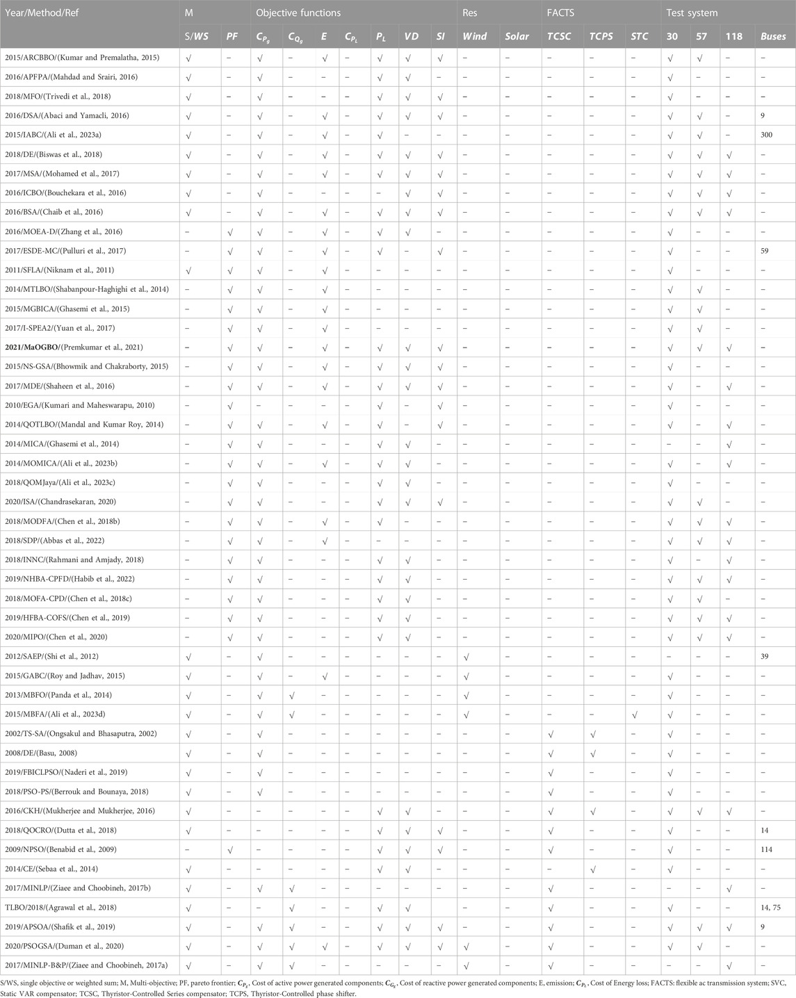
TABLE 1. CRUX of the literature review for the single and multi-objective OPF problem with and without integration FACTS devices.

1.1 Motivation

Table 1 clearly shows that Multiobjective EAs considering simultaneously minimization of highly conflicting objective functions such as active power cost of conventional thermal generators along with the uncertain cost of wind generators, cost of energy loss, and emission was not employed to solve. In addition, real-time simultaneous modeling of both the site and size of various FACTS devices such as static var compensator (SVC), thyristor-controlled series compensator (TCSC), and thyristor-controlled phase shifter (TCPS) has not been employed to solve multi-objective optimal power flow (MOOPF) problems. This is crucial to take into account since the placement and size of FACTS devices can have a big impact on the optimization goals, such as cost, emission reduction, and cost of energy loss. Therefore, the integration of both site and size modeling of FACTS devices into MOOPF solutions can potentially lead to more effective and efficient power system optimization. Single objective OPF is extensively researched in the literature, as shown in Table 1, taking into account technical, economic, and environmental objective functions. Compared to single objective OPF, MOOPF is more resilient to unpredictable factors like changes in load and the supply of renewable energy. In a single simulation run, multi-objective also offers a trade-off between several competing objective functions, which can assist decision-makers in optimizing the power system with improved overall performance and efficiency. Multiobjective optimization is important, particularly in the face of growing renewable energy integration, which can increase the complexity of power systems and create new challenges for system operators. It can also be used to reduce the environmental impact of power systems, by optimizing objectives such as reducing emissions or promoting renewable energy integration. This can help utilities to meet environmental targets and reduce their carbon footprint.

In recent years extremely efficient MOEAs such as Two-phase (ToP) (Liu and Wang, 2019), CCMO (Tian et al., 2020), C3M (Sun et al., 2022), and BiCo (Ali et al., 2023e) are implemented to solve mathematical optimization problems, they were not employed to solve mixed integer nonlinear MOOPF problem considering site and size of FACTS device and probabilistic wind generation. In the literature review, several of the multi-objective evolutionary algorithms (MOEAs) were examined. These MOEAs make use of the penalty function approach, a common method for dealing with restrictions that penalizes those who violate them. The selection of the penalty parameters has a significant impact on the approach’s efficacy. If the penalty coefficient is set too low, the algorithm may get stuck in an unfeasible region, and if it is set too high, the feasible space may be over-explored and the program may become stuck in local optima. A final non-dominated Pareto front solution that is not viable might also result from choosing the wrong penalty parameter. Therefore, in order to lead MOEAs for a real multi-objective problem with constraints, a suitable constraint management technique is needed. This looks for a broadly scattered Pareto front close to the global optimum after searching all of the physically possible space and escaping the infeasible zone. Additionally, the majority of writers in the literature examined state that their MOEAs are robust and have converged, producing a better Pareto front than other MOEAs, and they use pre-defined parameters for their MOEAs. Comparing many MOEAs is difficult, though, because each MOEA’s performance is heavily influenced by the data it collects and its pre-established settings.

1.2 Contributions

In this research, authors developed a stochastic model of wind power probability and used it to optimize the distribution of three different FACTS devices: the TCSC, the TCPS, and the SVC. As part of the optimization process, we take into account penalties and reserve costs associated with deviations from scheduled wind power output and determine the optimal placement and rating for these devices to achieve the lowest possible total cost of generation. Furthermore, we have carried out a case study to investigate the effects of wind power, uncertain load demand, and FACTS devices on the system. In order to determine the best location and size for FACTS devices and the integration of wind in power systems, the Multi-Objective Optimal Power Flow (MOOPF) problem formulation has been taken into consideration. This study makes a significant contribution by simultaneously taking into account a number of competing objective functions, such as the price of active power, emissions, and energy loss. The limited domination principle and the bidirectional coevolutionary (BiCo) algorithm are used to generate a large number of solutions in a single simulation run, allowing power system operators to make well-informed decisions that balance various factors. The suggested algorithm BiCo is able to deliver an evenly spaced and wide range of non-dominated solutions, allowing power system operators to choose the option that best matches their demands, according to a thorough examination and comparison of simulation data. In the proposed MOOPF formulation, optimal siting and allocation of FACTS devices are used to mitigate the limitations of wind generation, as discussed earlier, while wind integration can help to reduce emissions and the cost of conventional thermal generators. The proposed formulation also made significant contributions to model various conflicting two and three-objective functions of three study cases to solve deterministic and probabilistic MOOPF problems.

The rest of the paper is structured as; In Section 2 proposed FACTS devices are modeled, and in Section 3, the MOOPF problem is formulated. Section 4 discusses the constraint handling technique (CHT) and the framework proposed algorithm. The findings of the simulation are carefully evaluated and juxtaposed in Section 5. Section 6 contains the paper’s conclusion.

2 Modeling of FACTS devices

Improved power system efficiency is achieved with the use of FACTS devices. Utility companies can save money upgrading their current AC transmission system by switching to these substation-based controls, which have faster reactions against power flow fluctuation in transmission lines. Increased power transfer capability, improved voltage stability, faster reaction, lower transmission losses, and increased grid dependability are only some of the benefits of using FACTS devices in power system operation and management. When it comes to boosting the efficiency and dependability of power grids, FACTS devices are both adaptable and affordable. They can aid in lowering the environmental toll of producing and transporting electricity, thereby helping to satisfy rising demand. In general, the goals and limitations of the power system’s operation determine which FACTS devices are chosen for MOOPF. Power system efficiency, reliability, cost, and environmental effect can all benefit from the strategic placement of FACTS devices. Static Var Compensator (SVC), Thyristor-Controlled Series compensator (TCSC), and thyristor-controlled phase shifter (TCPS) are just a few examples of the many FACTS devices available. In this study, we apply SVC, TCSC, and TCPC to enhance power system performance in the face of variable wind integration. Figure 1 shows a conceptual diagram of power system integration.

FIGURE 1

FIGURE 1. The pi network of the Transmission line between bus i and k with the integration of SVC, TCSC, and TCPS.

2.1 Modeling OF SVC devices

SVC devices are important for managing the power flow of transmission lines because of their ability to modulate voltage by absorbing or producing reactive power into or out of the bus. For the purpose of mitigating voltage dips and keeping the system stable during transient occurrences, SVCs are utilized in MOOPF difficulties here to manage the voltage and offer reactive power compensation. By applying SVCs to MOOPF challenges, we can boost the power grid’s stability and security while increasing its efficiency and dependability across the board. Figure 1 is a schematic depicting the power distribution for the SVC model, showing how the kth bus receives power (Kumar and Premalatha, 2015; Mirsaeidi et al., 2023):

$B_{SVC}=B_C+B_L\left(\gamma \right)(1)$

$Q_{SVC}=-V_k^2{B}_{SVC}(2)$

The objective functions in MOOPF problems typically include minimizing the cost of generation and minimizing the transmission losses. By controlling the reactive power output of SVCs that is $Q_{SVC}$, these objectives can be achieved more efficiently and effectively. In the proposed MOOPF problems, SVCs are modeled as negative VAR generators across the PQ buses (Biswas et al., 2020).

2.2 Modeling of TCSC

TCSC consists of a thyristor-controlled reactor and a fixed series capacitor connected in parallel. The combined capacitive and inductive reactance of a TCSC, denoted by the symbol X_C and X_L, respectively, can be written as:

$X_{TCSC}\left(\gamma \right)=\frac{X_C{X}_L\left(\gamma \right)}{X_L\left(\gamma \right)-X_C}(3)$

Figure 1 displays the fixed model of TCSC that is installed on the line linking buses i and k. Upon integrating TCSC (as a changeable capacitive reactance) into the system, the modified reactance $\left(X_{eq}\right)$ of the transmission line is altered, as indicated by the following equation:

$X_{eq}=X_{ik}-X_{TCSC}=\left(1-\tau \right)X_{ik}(4)$

Whereas,

$\tau =\frac{X_{TCSC}}{X_{ik}}(5)$

The inductive reactance of the line is denoted by $X_{ik}$ and $\tau$ represents the degree of series compensation. The power flow equations (Basu, 2008; Biswas et al., 2020) for the line, which takes into account TCSC, can be formulated as:

$P_k^f=V_i^2{G}_{ik}{-V}_i{V}_k{G}_{ik}\cos \left({\delta }_i-{\delta }_k\right)-V_i{V}_k{B}_{ik}\sin \left({\delta }_i-{\delta }_k\right)(6)$

$Q_k^f=-V_i^2{B}_{ik}-V_i{V}_k{G}_{ik}\sin \left({\delta }_i-{\delta }_k\right)+V_i{V}_k{B}_{ik}\cos \left({\delta }_i-{\delta }_k\right)(7)$

$P_k^t=V_k^2{G}_{ik}-V_i{V}_k{G}_{ik}\cos \left({\delta }_i-{\delta }_k\right)+V_i{V}_k{B}_{ik}\sin \left({\delta }_i-{\delta }_k\right)(8)$

$Q_k^t=-V_k^2{B}_{ik}+V_i{V}_k{G}_{ik}\sin \left({\delta }_i-{\delta }_k\right)+V_i{V}_k{B}_{ik}\cos \left({\delta }_i-{\delta }_k\right)(9)$

Whereas, $G_{ik}$ and $B_{ik}$ are the conductance and susceptance of transmission line between buses i and k, can be computed as $G_{ik}=\frac{R_{ik}}{{\left[R_{ik}^2+\left(1-\tau \right)X_{ik}\right]}^2}$ and $B_{ik}=-\frac{\left(1-\tau \right)X_{ik}}{{\left[R_{ik}^2+\left(1-\tau \right)X_{ik}\right]}^2}$, respectively. ${\delta }_i$ and ${\delta }_k$ are the voltage angles at bus i and k.

2.3 Modeling of TCPS

Figure 1 depicts the arrangement of TCPS on the line between buses i and k. In case TCPS introduces a phase shift angle $\varphi$, the power flow equations for the line, using the equations given in references (Basu, 2008; Biswas et al., 2020), can be expressed as.

$P_k^f=\frac{V_k^2{G}_{ik}}{{\cos }^2\varphi }-\frac{V_i{V}_k}{\cos \varphi }\left[G_{ik}\cos \left({\delta }_i-{\delta }_k+\varphi \right)+B_{ik}\sin \left({\delta }_i-{\delta }_k+\varphi \right)\right](10)$

$Q_k^f=-\frac{V_i^2{B}_{ik}}{{\cos }^2\varphi }-\frac{V_i{V}_k}{\cos \varphi }\left[G_{ik}\sin \left({\delta }_i-{\delta }_k+\varphi \right)-B_{ik}\cos \left({\delta }_i-{\delta }_k+\varphi \right)\right](11)$

$P_k^t=V_k^2{G}_{ik}-\frac{V_i{V}_k}{\cos \varphi }\left[G_{ik}\cos \left({\delta }_i-{\delta }_k+\varphi \right)-B_{ik}\sin \left({\delta }_i-{\delta }_k+\varphi \right)\right](12)$

$Q_k^t=-V_k^2{B}_{ik}+\frac{V_i{V}_k}{\cos \varphi }\left[G_{ik}\sin \left({\delta }_i-{\delta }_k+\varphi \right)+B_{ik}\cos \left({\delta }_i-{\delta }_k+\varphi \right)\right](13)$

Whereas, in power flow equations $\varphi$ is the phase angle shift produced by TCPS.

3 Problem formulation

The proposed approach involves modeling the optimal placement and sizing of series and shunt FACTS devices, in addition to the optimal integration of wind turbines. The MOOPF is formulated to address this issue, which is a non-convex and non-linear problem (NLP) with multiple objective functions (M ≥ 2). The objective function is expressed as follows, without any loss of generality:

$\min F\left(\overrightarrow{x}\right)=\left[f_1\left(\overrightarrow{x}\right),f_2\left(\overrightarrow{x}\right),\dots ,f_M\left(\overrightarrow{x}\right)\right]\mathrm{s}.\mathrm{t}:g_i\left(\overrightarrow{x}\right)=0,i=\mathrm{1,2,3},\dots .,p{h}_j\left(\overrightarrow{x}\right)\le 0,j=\mathrm{1,2,3},\dots ,q\overrightarrow{x}\in \mathrm{\Omega }(14)$

While the objective functions are $f_1\left(x\right),f_2\left(x\right),\dots ,f_M\left(x\right)$ the equality constraints are $g_i\left(\overrightarrow{x}\right)$ and the inequality constraints are, $h_j\left(\overrightarrow{x}\right)$, respectively. Both $g_i\left(\overrightarrow{x}\right)$ and $h_j\left(\overrightarrow{x}\right)$ constraints define the feasible region and $\overrightarrow{x}$ is the decision vector. In the following subsections objective functions, equality and inequality constraints, and decision vectors are mathematically formulated. Table 2; Figure 2 provide details about the proposed network and single-line diagram of the simulation resistively.

TABLE 2

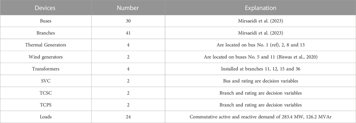
TABLE 2. Data of IEEE standard 30-BUS test system under study.

FIGURE 2

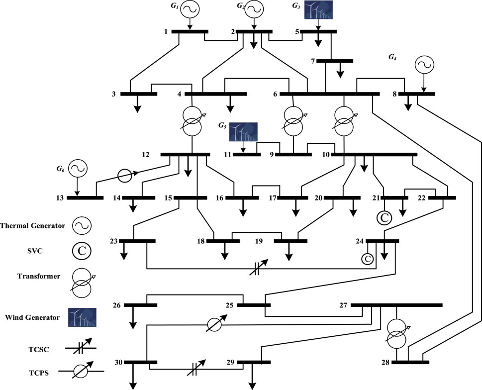
FIGURE 2. Adapted modified IEEE 30-bus test network.

3.1 Objective functions, constraints, and decision variables

The selection of objective functions in the MOOPF problem is based on the fact that these functions represent the primary concerns of power system operators and regulators. In this study, we have chosen these three Multiobjective functions to reflect the economic, environmental, and technical aspects of power system operation. The cost of generation is important for ensuring the economic viability of power system operation, while the emission cost reflects the need for reducing the environmental impact of power generation. The cost of energy loss is important for ensuring the efficient operation of the power system by minimizing transmission and distribution losses. Therefore, the selection of these multi-objective functions is based on their importance in achieving the overall objective of sustainable and efficient power system operation. By considering these objectives in a multi-objective optimization framework, the authors aim to provide a comprehensive solution that balances the trade-offs between these different objectives. Additionally, the integration of wind generation and the optimal location and sizing of FACTS devices are also incorporated into the MOOPF problem formulation.

3.2 Formulation of objective functions

3.2.1 Cost model

The cost of power generation $C\left(P_g\right)$ and reactive power produced by FACTs devices is given as;

$f_1={\displaystyle \sum _{sc=1}^{N_{SC}}}{∆}_{sc}{\displaystyle \sum _{i=1}^{N_G}}\left(C\left(P_{gt}\right)+C\left(P_{gW}\right)+C\left(FAC\right)\right)(15)$

Where, $N_{SC}$ and $N_G$ are the total number of scenarios and generators, ${∆}_{sc}$ shows the probability of each scenario. In this work cost of thermal generators $C\left(P_{gt}\right)$ is computed as:

$C\left(P_{gt}\right)=a+b{P}_G+c{P}_G^2(16)$

Where, $a,b,$ and $c,\mathrm{a}$ re the parameters (Mohamed et al., 2017) and $P_g$ is the output power of thermal generator. Cost of wind power generation $C\left(P_{gW}\right)$ is comprised of three components such as direct cost, reserve cost and penalty cost, given as:

$C\left(P_{gW}\right)=\underset{Directcost}{\underbrace{g_w{P}_{schW}}}+\underset{Reservecost\left(P_{gW}<P_{sched}\right)}{\underbrace{C_R\left(P_{schW}-P_{Wav}\right)}}+\underset{Penaltycost\left(P_{gW}>P_{sched}\right)}{\underbrace{C_P\left(P_{Wav}-P_{schW}\right)}}(17)$

Whereas; $g_w$ is the direct cost coefficient. The direct cost of wind generation refers to the expenses associated with the installation, operation, and maintenance of wind power facilities. Reserve cost $C_R$ refer to the cost of maintaining a reserve capacity of power generation to ensure that the power supply remains stable even when wind generation is variable. Since wind power generation is intermittent and unpredictable, it is necessary to have a reserve capacity to ensure that there is enough power supply to meet demand during periods of low wind generation. The reserve cost can be significant and may include the cost of backup power sources, such as natural gas generators or energy storage systems. On the other hand, the Penalty cost $C_P$ refer to the costs that wind generators may incur if they are unable to deliver the amount of electricity that they have committed to providing to the grid. These penalties can be levied by the grid operator as a way of incentivizing wind generators to meet their commitments and to ensure that there is enough electricity available to meet demand. These penalties can also add to the direct cost of wind generation and need to be taken into account when estimating the overall cost of wind energy projects. Therefore, considering the reserve and penalty costs of wind generators is important to ensure that the project is economically viable and to accurately estimate the total cost of wind generation. By taking these costs into account, the author can provide a more comprehensive analysis of the economic feasibility of a wind energy project. Reserve and penalty costs are calculated mathematically as:

$C_R\left(P_{schW}-P_{Wav}\right)=K_{RW}{\int }_0^{P_{schW}}\left(P_{schW}-p_W\right)\times {\pi }_w\left(p_W\right)d{p}_W(18)$

$C_P\left(P_{Wav}-P_{schW}\right)=K_{PW}{\int }_{P_{schW}}^{P_{Wr}}\left(p_W-P_{schW}\right){\pi }_W\left(p_W\right)d{p}_W(19)$

Whereas, $K_{RW}$ and $K_{PW}$ are the reserve and penalty cost coefficients and $P_{schW}$ and $P_{Wav}$ are scheduled and amiable wind power at the site. By accurately estimating wind power probabilities, power system operators can optimize the use of wind energy resources and ensure the reliable and efficient operation of the power system. Before computing the cost of wind generators, it is desirable to compute uncertainties in wind generation. This is because wind generation is highly variable and uncertain, and the actual output of wind generators can deviate significantly from their expected values. By quantifying the uncertainties in wind generation, power system operators can better estimate the expected output of wind generators and make more informed decisions about the deployment and operation of wind power plants. This can help minimize the economic cost of wind generation, ensure grid stability, and support the integration of renewable energy sources into the power system. The Weibull PDF is a probability distribution that is commonly used to model wind speed. It is characterized by two parameters: the shape parameter, b, and the scale parameter, a. The PDF of the Weibull distribution (Shi et al., 2012; Biswas et al., 2017) is given by the following equation:

${\Delta }_{\nu }\left(v\right)=\left(\frac{b}{a}\right){\left(\frac{v}{a}\right)}^{\left(b-1\right)}\times e^{\left[-{\left(\frac{v}{a}\right)}^b\right]}(20)$

The present study makes use of the wind turbine model developed in (E. E.-E. 3.000, 2023). The E82-E4 has a rotor diameter of 82 m and a hub height of 108 m. The wind turbine uses a direct-drive generator, which eliminates the need for a gearbox and improves reliability and efficiency. The E82-E4 also features a pitch-controlled rotor system, which allows the blades to be adjusted to optimize power production under different wind conditions. The wind turbine has a cut-in $v_{in}$ wind speed of 3 m/s, rated $v_r$ wind speed of 15 m/s and a cut-out $v_{out}$ wind speed of 25 m/s. The E82-E4 is designed for use in onshore wind farms and is suitable for low to medium wind speeds. The proposed wind farm comprising 25 turbines each of 3 MW is connected to bus 5, and 20 turbines of 3 mW are connected to bus 11. The power generated by each wind turbine is calculated using the following formula:

$p_W\left(v\right)=\left\{\begin{array}{l}0,for\nu <v_{in}andv>{\nu }_{ouT}\\ p_{wr}\left(\frac{v-{\nu }_{in}}{{\nu }_r-v_{in}}\right)for{v}_{in}\le v\le v_r\\ p_{wr}for{v}_r<\nu \le v_{ouf}\end{array}\right.(21)$

Equation 21 clearly demonstrates that the power generated by a wind turbine is a piecewise function of wind speeds. Following are the calculations for the likelihood of wind power in these various zones:

${\pi }_w\left(p_W\right)\left\{p_w=0\right\}=1-{\mathrm{e}}^{\left[-{\left(\frac{v_{in}}{\alpha }\right)}^{\beta }\right]}+{\mathrm{e}}^{\left[-{\left(\frac{v_{ou1}}{\alpha }\right)}^{\beta }\right]}(22)$

${\pi }_w\left(p_W\right)\left\{p_w=p_{wr}\right\}={\mathrm{e}}^{\left[-{\left(\frac{v_r}{\alpha }\right)}^{\beta }\right]}-{\mathrm{e}}^{\left[-{\left(\frac{v_{out}}{\alpha }\right)}^{\beta }\right]}(23)$

${\pi }_w\left(p_W\right)=\frac{\beta \left(v_r-v_{in}\right)}{{\alpha }^{\beta }*p_{wr}}\left[{v_{\iota n}+\frac{p_w}{p_{wr}}\left(v_r-v_{in}\right)}^{\beta -1}\right]\times {\mathrm{e}}^{\left[-{\left(\frac{v_{in}+\frac{p_w}{p_{wr}}\left(v_r-v_{in}\right)}{\alpha }\right)}^{\beta }\right]}(24)$

Moreover, in this study the installation cost of cost of FACTs devices $C\left(FAC\right)$ as given (Shehata et al., 2022) is computed as;

$C\left(FAC\right)=C\left(SVC\right)+C\left(TCSC\right)(25)$

Whereas, $C\left(SVC\right)$ and $C\left(TCSC\right)$ are the installation cost of SVC devices and TCSC devices and in this study these costs are nonlinear quadratic cost and computed as;

$C\left(SVC\right)=0.0003S^2+0.3051S+127.38(26)$

$C\left(TCSC\right)=0.0013S^2-0.7130S+133.73(27)$

Where, S is the MVAr operating range of FACTs devices.

3.2.2 Emissions generated by thermal generators

Considering greenhouse gas emissions as one of the objective functions in the optimization of power systems can have significant environmental, regulatory, financial, and technological benefits. Greenhouse gases particularly carbon dioxide (CO₂) is one of the primary contributors to global climate change. By reducing greenhouse gas emissions, power systems can play a significant role in mitigating the effects of climate change and preserving the planet for future generations. The mathematical derivation to compute emissions generated by thermal generators depends on the specific pollutant being considered and the type of fuel being used. In general, emissions from thermal generators can be estimated by using emission factors that relate the number of pollutants emitted to the amount of fuel consumed or energy generated. The basic equation for estimating emissions $E\left(P_{gt}\right)$ from thermal generators is:

$f_2={\displaystyle \sum _{sc=1}^{N_{SC}}}{∆}_{sc}{\displaystyle \sum _{i=1}^{NG}}\left[\left({\alpha }_i+{\beta }_i{P}_{Gi}+{\gamma }_i{P}_{Gi}^2\right)+{\omega }_i{e}^{\left({\mu }_i{P}_G\right)}\right](28)$

Where the constants for the cost and emission of the thermal generators are ${\mathrm{\alpha }}_{\mathrm{i}},{\mathrm{\beta }}_{\mathrm{i}},{\mathrm{\gamma }}_{\mathrm{i}},{\mathrm{\omega }}_{\mathrm{i}}$ and ${\mathrm{\mu }}_{\mathrm{i}}$ (Bhowmik and Chakraborty, 2015).

3.2.3 Cost of power loss

The cost of energy loss represents the economic cost of the energy that is lost as it flows through the power system due to resistive losses in transmission and distribution lines and transformers. By including the cost of energy loss term, the optimizer will therefore seek to balance the generation and transmission of power in a way that minimizes energy losses and overall system cost. In MOOPF problems, the cost of energy loss can be computed as;

$P_{Loss}={\displaystyle \sum _{sc=1}^{N_{SC}}}{∆}_{sc}{\displaystyle \sum _{i=1}^{Nb}}{\displaystyle \sum _{k=i+1}^{Nb}}{G}_{ik}\left[V_i^2+V_k^2-2V_i{V}_k\mathit{cos}{\delta }_{ik}\right](29)$

Whereas, ${\delta }_{ik}={\delta }_i-{\delta }_k$, $V_i$ is the complex voltage at bus i.

$f_3=a*P_{Loss}(30)$

Where a is the energy loss coefficient which is 0.1 $/kWh.

3.3 Equality and inequality constraints

The equality constraint $g\left(\overrightarrow{x}\right)$ are:

$P_{Gi}-P_{Di}-V_i{\displaystyle \sum _{k=1}^{NB}}{V}_k{Y}_{ik}\cos \left({\theta }_{ik}+{\delta }_i-{\delta }_k\right)=0,\forall i\wedge k\in NB(31)$

$Q_{Gi}-Q_{Di}{V}_i{\displaystyle \sum _{k=1}^{NB}}{V}_k{Y}_{ik}\sin \left({\theta }_{ik}+{\delta }_i-{\delta }_k\right)=0,\forall i\wedge k\in NB(32)$

where $P_{Gi}$ and $Q_{Gi}$ are real and reactive generation. $P_{Di}$ and $Q_{Di}$ are load demands, at bus i. $Y_{ik}$ is branch admittance of ikth line, and ${\theta }_{ik}$ is the angle. NB shows the total number of buses. On the other hand, inequality constraint $h\left(\overrightarrow{x}\right)$ for the OPF problem are Figured as;

$P_{gi}^{\mathit{min}}<P_{gi}<P_{gi}^{\mathit{max}},\forall i\in N_G(33)$

$Q_{gi}^{\mathit{min}}<Q_{gi}<Q_{gi}^{\mathit{max}},\forall i\in N_G(34)$

$V_{gi}^{\mathit{min}}\le V_{gi}\le V_{gi}^{\mathit{max}},\forall i\in N_G(35)$

$V_L^{\mathit{min}}\le V_L\le V_L^{\mathit{max}},\forall L\in N_L(36)$

$S_l\le S_l^{\mathit{max}},\forall l\in N_l(37)$

${Tap}_T^{\mathit{min}}\le {Tap}_T\le {Tap}_T^{\mathit{min}},\forall T\in N_T(38)$

$Q_{SVC}^{\mathit{min}}\le Q_{SVC}\le Q_{SVC}^{\mathit{max}},\forall j\in N_{SVC}(39)$

${\tau }_{TCSCm}^{\mathit{min}}\le {\tau }_{TCSCm}\le {\tau }_{TCSCm}^{\mathit{max}},\forall m\in N_{TCSC}(40)$

${\Phi }_{TCPS}^{\mathit{min}}\le {\Phi }_{TCPS}\le {\Phi }_{TCPS}^{man},\forall n\in N_{TCPS}(41)$

The limits of active and reactive power generation for thermal and wind generators are described by Eqs. 33, 34, respectively. These equations apply to all generator buses, with the total number of generators or generator buses being denoted as $N_G$. Eq. 35 specifies the voltage constraint for generator buses, while Eq. 36 applies to the voltage constraint for load buses. The line capacity constraint is expressed in Eq. 37. Eq. 38, where N_T stands for the number of transformers, specifies the upper and lower bounds for the transformer tap settings. In Eqs 39–41, the constraints for FACTS devices, including SVC, TCSC, and TCPS, are given, respectively. It is important to highlight that satisfying the equality constraints in the optimal power flow (OPF) problem can only be done by attaining power flow convergence. Using the MATPOWER (Zimmerman et al., 2011), we apply the Newton-Raphson (NR) technique for calculating power flow (Zimm et al., 2009). A proper constraint-handling strategy is needed to guarantee that these restrictions are observed. In Section 4, we dive deeper into how an optimization algorithm can be used in tandem with a constraint handling technique.

3.4 Decision variables

The study presented in this paper considers all load scenarios and wind generation probabilities and computes their upper and lower bounds. The objective functions and constraints for each of these scenarios are then integrated into a single, complicated master issue, where they are each considered as a separate island in a stacked network of all the scenarios. When taking into account wind and probabilistic load models, using a single solution for all the MOOPF problem scenarios can have benefits such as faster computation, higher accuracy, increased flexibility, better system planning, and easier integration of intertemporal reserve constraints. The master OPF problem offers a single solution for all scenarios that may be utilized to make decisions in real-time, allowing for increased flexibility in the management of power systems. In situations where the variability of wind and load demand may affect the stability of the power grid, such as the management of intertemporal reserve constraints for fixed zonal reserves, security constraint (NPF) analyses, and multipored scheduling of renewable energy systems, this can be especially crucial. This paper defines the decision vector for the OPF problem, represented as $\overrightarrow{x}$:

$\mathit{x}=\left[P,V,\tau ,{SVC}_p,SV{C}_r,TCS{C}_p,TCS{C}_r,TCP{S}_p,TCP{S}_r\right](42)$

Where GN, TN, and $\tau$ are the number of generators, P and V are the output power of the generators and the voltage at the generator bus, respectively, and is the transformer tap ratio. The discrete positions and continuous ratings of SVC, TCSC, and TCPS are represented by subscripts p and r. The decision variable in the suggested formulation was made up of mixed-integer variables.

4 Constraint domination principle and MOEAS

Due to its limited feasible search area and constraints in both the objective and control variable spaces, the MOOPF issue is a real-world constrained multi-objective optimization problem that poses difficulties for existing MOEAs. This work suggests adopting the bidirectional co-evolutionary (BiCo) constrained MOEA, which manages constraints by applying the constraint domination principle (CDP).

4.1 A pareto front with a pareto set

A feasible zone is one where all decision vectors have zero constraint violation (CV) $.$ The Pareto front (PF) is the set of all Pareto optimal solutions in objective space. Pareto optimal solutions (PS) are the set of all solutions that correspond to viable regions.2).

4.2 Pareto dominance

The concept of Pareto dominance states that if two decision vectors ${\overrightarrow{x}}_u$ and ${\overrightarrow{x}}_v$ are considered, and for all objective functions, $f\left({\overrightarrow{x}}_u\right)$ has a value that is less than or equal to of $f\left({\overrightarrow{x}}_v\right)$ but for at least one objective function $j$, $f_j\left({\overrightarrow{x}}_u\right)$ is less than $f_j\left({\overrightarrow{x}}_v\right)$, then ${\overrightarrow{x}}_u$ is said to dominate ${\overrightarrow{x}}_v$, and ${\overrightarrow{x}}_u$ is considered non-dominated or better than ${\overrightarrow{x}}_v$.

4.3 Constraint domination principle (CDP)

The Constraint Domination Principle (CDP), proposed in (Deb et al., 2002), is a simple and efficient constraint handling technique (CHT) used in this paper. It compares pairs of individuals using the following rules:

If both solutions ${\overrightarrow{x}}_u$ and ${\overrightarrow{x}}_v$ are infeasible, select ${\overrightarrow{x}}_u$ if $CV\left({\overrightarrow{x}}_u\right)<CV\left({\overrightarrow{x}}_v\right)$.

${\overrightarrow{x}}_u$ is feasible and ${\overrightarrow{\mathrm{x}}}_{\mathrm{v}}$ is infeasible, select the feasible one i.e., ${\overrightarrow{x}}_u$.

If both ${\overrightarrow{x}}_u$ and ${\overrightarrow{x}}_v$ are feasible, then select ${\overrightarrow{x}}_u$ if for all the objective functions $f_i\left({\overrightarrow{x}}_u\right)\le f_i\left({\overrightarrow{x}}_v\right)$.

4.3.1 Multi-objective bidirectional co-evolutionary algorithm (BICO)

The existence in the MOOPF problem makes it difficult for MOEAs to achieve well-converged and uniformly dispersed PF. But the majority of MOEAs favor workable solutions, which can cause two problems. First, people can become trapped in their local, optimally viable areas. Second, since the population only expands from the viable side, the search for space exploration might be restricted. The population may become imprisoned in local feasible or optimal feasible regions as a result of the conventional strategy of only optimizing feasible solutions, which restricts its capacity to effectively move the solutions towards the real or global PF. To overcome these issues, a bidirectional co-evolutionary (BiCo) algorithm (Ali et al., 2023e) along with the integration of CDP (Deb et al., 2002) is proposed in this paper, which coevolves both feasible (main) and infeasible (archive) populations to drive the solutions towards the PF. This is accomplished by looking at the search space from both the feasible and impractical sides. The archive population is also updated using a novel angle-based density (AD) selection strategy that preserves the diversity of the search space, makes it easier to find more feasible regions, and keeps the infeasible solutions that are close to the PF.

The BiCo can be explained in four steps. Firstly, an initial population is created randomly and the objective functions and overall constraint violation (CV) of each population are evaluated. The second step involves generating an offspring population ($Q_t$) by collaborating and interacting between the main (feasible search space) and archive (promising infeasible solutions) populations to produce high-quality offspring. Binary tournament selection is used to select parents for the mating pool. If the length of the archive population ($‖A_t‖$) is smaller than the population size N, parents are chosen from the combined population of the main ($P_t$) and archive ($A_t$) populations. Otherwise, the selection of parents is done alternatively by comparing the main and archive populations based on constraint violation and angle-based-density (AD), respectively. To select parent $p_1$, two solutions $x_1$ and $a_1$ are randomly selected from $P_t$ and $A_t$, respectively, and the one with the smaller CV value is chosen. To choose $p_2,x_2$ and $a_2$ are picked randomly from $P_t$ and $A_t$, respectively, and the one with the larger AD value is chosen. The proposed algorithm calculates AD as follows:

In the opening, normalize the objective function space, say jth solutions of objective functions $F_i^{\prime }\left(v_j\right)=\left(f_1^{\prime }\left(v_j\right),f_2^{\prime }\left(v_j\right),\dots ,f_m^{\prime }\left(v_j\right)\right)$ using ideal $Z_{\mathit{min}}^i$ and nadir $Z_{\mathit{max}}^i$ points in the combined population ${\mathcal{U}}_t$ according to;

$f_i^{\prime }\left(x_j\right)=\frac{f_i-Z_{\mathit{min}}^i}{Z_{\mathit{max}}^i-Z_{\mathit{min}}^i},i=\mathrm{1,2},\dots ,m(43)$

After that vector angle between $F^{\prime }\left(x_j\right)$ and $F^{\prime }\left(x_k\right)$ solutions selected from ${\mathcal{U}}_t$ is computed as

${\theta }_{x_j,x_k}^{\prime }=\arccos \left|\frac{{\mathit{F}}^{\prime }\left(x_j\right)\bullet {\mathit{F}}^{\prime }\left(x_k\right)}{‖{\mathit{F}}^{\prime }\left(x_j\right)‖‖{\mathit{F}}^{\prime }\left(x_k\right)‖}\right|where{x}_k\in {\mathcal{P}}_t\cap x_k\ne x_j(44)$

Next, each solution is ranked based on the angle between them. The larger the angle, the higher the rank of the solution, making it a promising candidate for mating selection. The third step involves updating the main population $P_{t+1}$, which is responsible for driving the search toward the PF from the feasible side of the search space. To do this, the main population is combined with the offspring population $Q_t$, and solutions are divided into feasible $S_1$ and infeasible $S_2$ sets. If the number of feasible solutions in $S_1$ is less than the population size N, then the first ($N-S_1$) infeasible solutions from the sorted set $S_2$ are selected. If the number of feasible solutions in $S_1$ is greater than N, non-dominated sorting is applied to $S_1$ to obtain the PF of different ranks, such as ${\mathcal{F}}_1,\dots ,{\mathcal{F}}_k$, and so on, where ${\mathcal{F}}_1$ is the highest rank. The solutions with the highest rank are assigned to $P_{t+1}$, followed by the second-highest rank, and so on until the size of $P_{t+1}$ is equal to N or greater than N. If the size of $P_{t+1}$ exceeds N, then the crowding distance (CD) operator is used to eliminate some of the solutions in the last front (Deb et al., 2002). Updating the archive population for the upcoming iteration is the fourth and last stage $A_{t+1}$, it creates non-dominated, impractical solutions in order to increase the Pareto front’s variety (Ali et al., 2023e). The algorithm considers CV as an additional objective function $M+1^{th}$, making the original constrained problem as an unconstrained multi-objective problem, given as:

$minF\left(x\right)={\left(f_1\left(x\right),f_2\left(x\right),\cdots ,f_m\left(x\right),CV\left(x\right)\right)}^T(45)$

This helps in generating promising non-dominated infeasible solutions. Next, the solutions are ranked using ND sort (Deb et al., 2002) to determine the PF, and capable infeasible solutions are selected based on CV (M+1 objective function) and AD as described in Eq. 39. Figure 3 displays the flow diagram for the proposed algorithm.

FIGURE 3

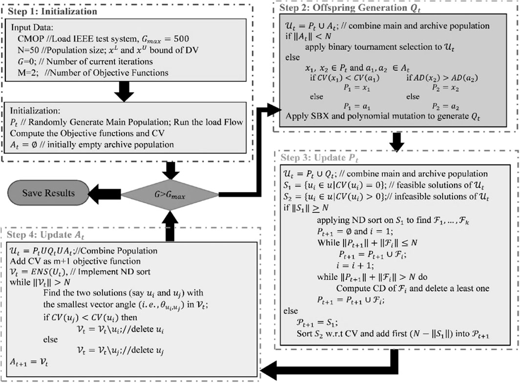
FIGURE 3. Flow diagram of the proposed algorithm.

5 Simulation results and discussion

In this paper, we consider the effectiveness of the proposed algorithm by evaluating it on the IEEE standard 30-bus test system. We provide detailed data of the test network as shown in Table 2 and proposed problem formulation in Section 3. Additionally, we implement four state-of-the-art MOEAs, including NSGAII (Deb et al., 2002), CCMO (Tian et al., 2020), ToP (Liu and Wang, 2019), and C3M (Sun et al., 2022), to solve the MOOPF problem. We present simulation results of all the algorithms applied to the MOOPF case studies and analyze and discuss them in this section. The formulation of objective functions in the MOOPF problem is based on the fact that these functions represent the primary concerns of power system operators and regulators. To highlight the technical, economic, and environmental facets of power system operation, we have selected three study examples with three conflicting objective functions with and with cost of FACTS devices. The proposed study cases without cost of FACTs devices:

• Case 1a: Cost of active power generation $C\left(P_g\right)$ from Eq. 15 vs. emission rate $E\left(P_{gt}\right)$ from Eq. 25.

• Case 2a: Cost of active power generation $C\left(P_g\right)$ from Eq. 15 vs. Cost of power loss $C\left(P_L\right)$ from Eq. 28

• Case 3a: All three objective functions $C\left(P_g\right)$ vs. $E\left(P_{gt}\right)$ vs. $C\left(P_L\right)$

The proposed study cases with cost of FACTs devices:

• Case 1b: Cost of active power generation $C\left(P_g\right)$ from Eq. 15 vs. emission rate $E\left(P_{gt}\right)$ from Eq. 25.

• Case 2b: Cost of active power generation $C\left(P_g\right)$ from Eq. 15 vs. Cost of power loss $C\left(P_L\right)$ from Eq. 28

• Case 3b: All three objective functions $C\left(P_g\right)$ vs. $E\left(P_{gt}\right)$ vs. $C\left(P_L\right)$

Each case study is applied to find the optimal site and size of FACTS devices with the integration of wind generation along with the consideration of deterministic and probabilistic scenario-based load variation. User-defined parameters of each algorithm are adopted from their original papers. However, in deterministic study situations, the population size and the maximum number of function evaluations are 40 and 20,000, respectively, whereas in probabilistic study cases, they are 40 and 50,000. Here, deterministic cases are merely altered to show how much better and more efficient the suggested approach is compared to the most recent state-of-the-art MOEAs. Solution of proposed study case has been found on the platform of MATLAB 2021b core i7 PC using version 9.10.

5.1 Allocation of FACTS devices in MOOPF problem with and without cost of FACTS devices

In the following subsections, we have conducted a comparison between the outcomes of our suggested algorithm and those of current advanced MOEAs. Fixed parameters of proposed algorithm have chosen from their original study, and population sizes and the maximum function evaluation of each algorithm remains fixed, allowing for a fair comparison between the proposed approach and existing Multi-Objective Evolutionary Algorithms (MOEAs). The selection of minimum and maximum values for each objective function and the Hypervolume Indicator (HVI) will be discussed in the following subsections. Additionally, each algorithm is run independently 20 times for each case to enable statistical comparison. The comparison between the proposed algorithm and other algorithms will be based on the best, worst, and mean values of the HVI. To ensure a fair comparison with regard to constraints, each algorithm is combined with the CDP constraint handling technique. As outlined in Section 4, the standard approach for integrating the CDP method is to be utilized at the stage of selecting population members for the next-generation.

5.1.1 Selection of best PF based on statistics of HVI and minimum values of objective functions

In a single simulation run, MOEAs seek to find high-quality non-dominated solutions. The goal of MOEAs is to produce non-dominated solutions with improved convergence, variety, evenness, and maximum spread. The effectiveness of the non-dominated solutions obtained using MOEAs is evaluated using these variables. Several performance criteria have already been developed to allow a fair comparison of MOEAs. In this work, the convergence and diversity of distinct MOEAs are assessed using a performance metric called the hypervolume indicator (HVI) (Deb et al., 2002). The genuine Pareto front (PF), which is required by the HVI metric, should ideally be close to the nadir point. The PF with the highest HVI is considered the best when evaluating different PFs for a certain situation. For all situations based on HVI, we outlined in Table 3 the statistical performance of the proposed algorithm and other cutting-edge MOEAs, such as NSGAII (Deb et al., 2002), CCMO (Tian et al., 2020), ToP (Liu and Wang, 2019), and C3M (Sun et al., 2022).

TABLE 3

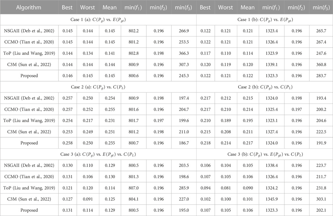
TABLE 3. Simulation results based ON HVI and extreme values of objective functions of all the study cases.

For each study case across twenty independent runs, Table 3 summarizes the statistical results of HVI (maximum, minimum, mean, and minimum value of each objective functions) of with and without cost of FACTS devices, highlighting the best outcomes. Table 3 demonstrates that in most of the study cases compared to HVI value, BiCo outperforms compared to all other algorithms. According on statistical data, the proposed algorithm outperformed the majority of MOEAs. In addition, extreme values of objective function optimal compromise solutions are viewed as the lowest among all MOEAs. That demonstrates the ability of the suggested approach to discover widespread PF. Also, in extremely complicated case 3a and 3b proposed algorithm outperforms compared to other MOEAs. Moreover, ToP consistently fails to find a higher value of HVI. C3M (Sun et al., 2022) gives better statistical results after that proposed algorithm. While PF of ToP is the trap into local optimum when determining the minimum values of each OF in all circumstances, it is also concluded that minimum values of objective functions in table demonstrate that BiCo always provides a well-distributed and wide range of objective function values. The final non-dominated solutions for each of the algorithm’s scenarios are shown in Figure 4 alongside the responses from the other MOEAs.

FIGURE 4

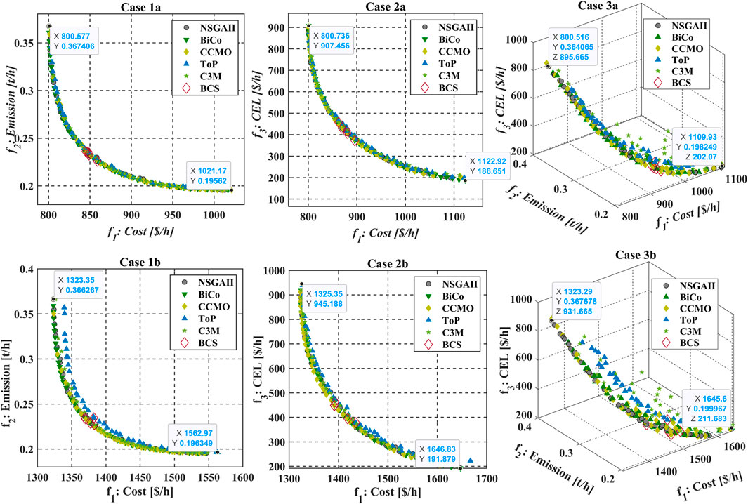
FIGURE 4. Comparison of best PFs of State-of-the-art MOEA with the proposed Algorithm.

Algorithms that produce Pareto fronts that are widely spread, evenly spaced, and well-converged in comparison to most techniques. Most of the time, ToP and NSGAII become trapped in locally optimum solutions. The visualization in Figure 4 shows that the suggested approach is capable of locating non-dominated, broadly spread, and evenly spaced solutions. Figure 4 also displays extreme values of non-dominated solutions produced by the suggested technique for improved visibility. A difficult optimization issue is one that has both discrete and continuous variables. It is important to emphasize that during the initial search phase, algorithms are driven by constraint-handling strategies and look for workable solutions. Once possible ones have been identified, the quality of the replies improves within the feasible range. Within a few hundred function evaluations, all algorithms in the investigated system found the feasible zone.

From the statistical values shown in Table 3 and from the final PF shown in Figure 4 these does not clearly shows that the performance of which algorithm in most of the independent runs find the better solution. Therefore, box chart for all the independent runs is as shown in Figure 5 clears that the proposed algorithm in most of the study cases outperforms compared to the other cases. Box chart give the statistical information of all the twenty independent runs (called sample data). Each box comprised of HVI values of all the independent runs of each algorithm. Moreover, line inside the box is called median, edges of the box called upper and lower quartiles. These quartiles also give the information about standard deviation (SD), larger the box areas more the SD and vice versa. The lines that extend above and below each box are called whiskers. Whiskers in box plot connects the quartiles to the minimum and maximum values of HVI. Notches in the box is used to compare the median of multiple boxes in the plot. Box charts whose notches do not overlap have different medians at the 5% significance level. In the Box chart bubble shows the outlier HVI value and these are more than 1.5 of interquartile range of bx. From the box chart it clearly shown that in all the runs proposed algorithm always converges and widely distributed solutions.

FIGURE 5

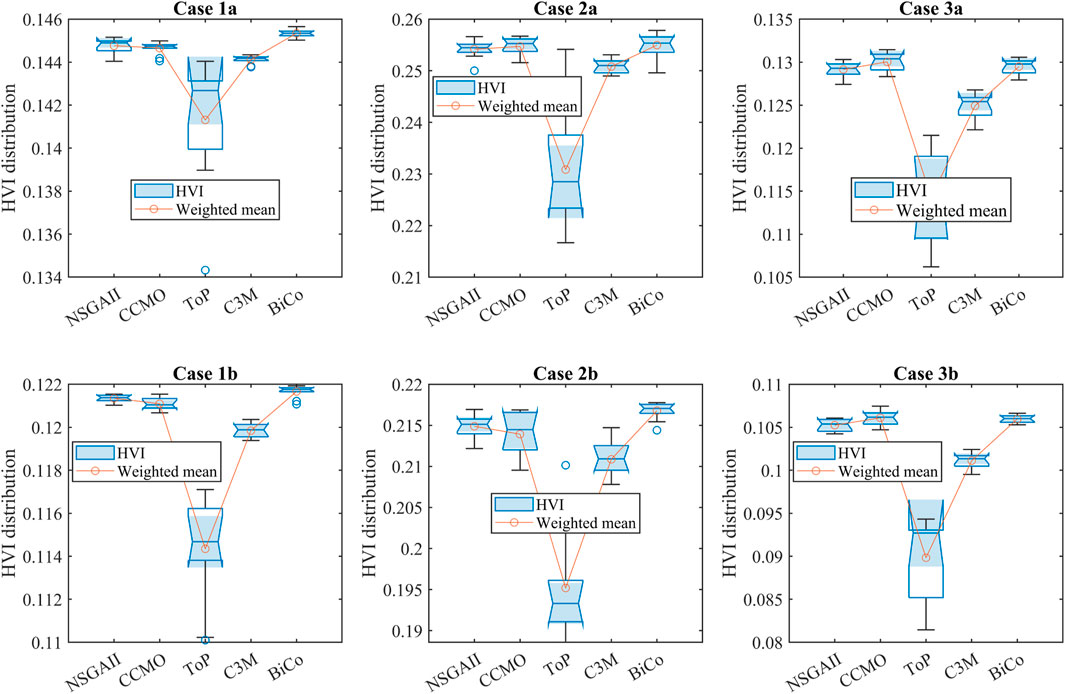
FIGURE 5. HVI distribution of all the cases of all the algorithms comparison with proposed algorithm.

5.1.2 Selection and analysis of best compromise solution (BCS)

There are 27 decision variables in the deterministic MOOPF problem, some of which pertain to where FACTS devices are installed. These variables are comprised of continuous and integer and the proposed MOOPF problem I s mixed integer nonlinear problem, integer variables correspond to location of TCSC/TCPS or SVC branch or bus numbers. Each FACTS device is subject to two sets of control variables: location and device rating. The location variable is rounded to the nearest integer before the power flow analysis, although it may become a fraction throughout the optimization process. FACTS devices are deployed instead of SVC on generator buses because of the potential for reactive power exchange. In addition, tap-changing transformers are not installed on branches with TCSC or TCPS, and no more than one FACTS device is installed in a given site. Transformer taps are taken to be discrete variables. The case studies’ range of probable tap settings is 0.90–1.10 p. u. During the search phase, the control variables for the transformer taps are rounded to the nearest multiple of 0.02 p. u. SVC can deliver or absorb reactive power up to 10 MVAr, but TCSC can lower.

Line reactance by up to 50% when it is installed. Angle adjustment for the phase shifter (TCPS) is possible between −5° and +5°. In most of cited papers available in the literature, the reactive power capacities of wind generators range from roughly −0.4 p. u. to 0.5 p. u. The BCS (Best Compromise Solution) is obtained through the use of a fuzzy decision approach, as described in reference (Abbas et al., 2022). This approach involves first calculating the membership function $\left({\mathrm{\mu }}_{\mathrm{m}}^{\mathrm{k}}\right)$ for the objective.

${\mu }_m^k=\left\{\begin{array}{ll}1& for{f}_m^k\le f_m^{\mathit{min}}\\ \frac{f_m^{\mathit{max}}-f_m^k}{f_m^{\mathit{max}}-f_m^{\mathit{min}}}& for{f}_m^{\mathit{min}}<f_m^k<f_m^{\mathit{max}}\\ 0& for{f}_m^k\ge f_m^{\mathit{max}}\end{array}\right.(46)$

The calculation of the membership function ${\mu }_m^k$ involves the use of parameters m and k, which represent the number of objective functions and final non-dominated solutions, respectively. The fitness value $f_m^k$ is also used in this calculation. Once the membership function is computed, it is then normalized to obtain the normalized membership function ${\mathrm{\mu }}^{\mathrm{k}}$.

$\overline{f}\left(x\right)={\displaystyle \sum _{i=1}^m}{\stackrel{\sim }{f}}_i\left(x\right)(47)$

The value of $N_d$ represents the number of solutions in the final PF (Pareto Front). The BCS can be determined by finding the index with the highest ${\mu }^k$ value and are shown in Figure 4 of diamond shape. Moreover, Table 4 displays the decision variables and objective function values of all the cases with and without cost of FACTS devices. Table 4 shows that the decision variables in all three study cases are within the desirable range. With the decision variable settings shown in Table 4 for Case 1a, where the cost of active power generation and emission are the objective functions, the proposed algorithm achieves costs of 848.9 ($/h) and emissions of 0.232 (t/h). The optimal siting of SVCs is located at buses 21 and 24 with the rating of 8.267 and 8.4029 respectively. Whereas the siting of TCSC and TCPS (branch number and the branch connected between the buses are also shown in Table 4). On the other hand, in Case 1b, where along with the cost of active power generation, cost of FACTS devices is also incorporated and emission are the objective functions, the proposed algorithm achieves costs of 1369.1 ($/h) and emissions of 0.234 (t/h). The optimal siting of SVCs is located at buses 8 and 13 with the rating of −9.97 and −9.92 MVAr respectively. Whereas the siting of TCSC and TCPS (branch number and the branch connected between the buses is also shown in Table 4).

TABLE 4

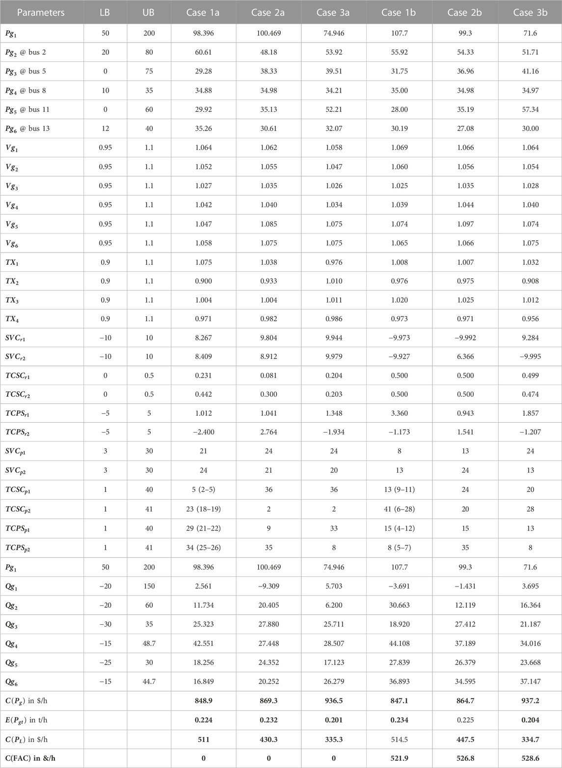
TABLE 4. Best compromise solutions for all cases using the proposed algorithm.

In both of the Cases 2a and 2b, only the direct cost of the wind generators (placed at buses 5 and 11) is taken into account in deterministic instances. The minimal value of the cost of active power generation achieved by the suggested algorithm is 869.3 ($/h) in Case 2a, and with slightly less cost of active power generation 864.7 ($/h) in case 2b. Whereas second objective function in Case 2a and 2b is the minimum value of the cost of energy loss is 430.3 and 447.5 ($/h) respectively. Cost of energy loss emphasize to decrease active power generation of all the thermal generators with the decrease in bus voltage level and hence emission in case 2a and 2b is reduced compared to case 1a and 1b. Form this comparison it clear to identify that cost of energy loss is the important objective function to control emission. In case 3a and 3b, all the tri objective functions are equally emphasized to find the decision vectors. Decision variables in both of the case 3a and 3b shown that the all the objective functions are better compared to case 1a, 1b and 2a, 2b. In Case 3a (without cost of FACTS devices), three objective functions such as the cost of active power generation, emission rate, and cost of energy loss are simultaneously minimized without considering the cost of FACTS devices. The values of objective functions obtained by the proposed algorithm are 936.5 ($/h), 0.201 (t/h), and 335.3 ($/h).

Whereas, in Case 3b, the values of objective functions obtained by the proposed algorithm are 937.2 ($/h), 0.204 (t/h), and 334.3 ($/h), which are marginally more than the values obtained in Case 3a. Computing the location of FACTS devices along with their ratings can provide significant benefits to power system planners, operators, and customers. By optimizing the installation of these devices, the power system can operate more efficiently, reliably, and cost-effectively. For FACTS devices to be as effective as possible, their ideal placement within a power system must be determined. Through optimization techniques, the location of FACTS devices can be determined in such a way that the power system can be operated at its highest efficiency, reliability, and stability. Currently, FACTS devices are frequently added to networks to improve their ability to handle higher loads. The placement of these devices is strategically optimized to minimize real power loss in the network and maximize its loading capacity. This is why Case 2 and 3, which aims to reduce the cost of real power loss in the network, is implemented. The need for an aim that takes into account both the cost of emissions and the cost of energy loss is therefore larger. Figure 6 displays the voltage profiles of all the study cases a) without considering the cost of FACTS devices and (b) considers the cost of FACTS devices.

FIGURE 6

FIGURE 6. Optimal setting of the bus voltages.

Figure 6 shows that compared to base case, voltage profile of all the study cases is better to seem. As compared to Case 1a, 2a and 3a, obtained voltage level of Case 3a is best and the similar situation is also shown in Case 1b, 2b and 3b. How when comparing the voltage profile between Cases a and b (such as with and without considering the cost of FACTS devices), Case 1b, 2b and 3b are seems better compared to Case 1a, 2a and 3a. All the voltage waveforms shown in Figures 6A, B are within desireable limit that highlights performance of the proposed MOEA with the integration of constraint domination principle. The aim of displaying the voltage profiles is to exhibit how the algorithm adheres to the limits the critical constraint on the voltage of PQ and PV buses. Simulation results shown in Table 4 further demonstrates how the suggested algorithm optimizes FACTS device placement and ratings to reduce generation costs, emission rates, and power loss costs with and without considering cost of FACTS devices. Previous works had fixed placements for the devices in the network, frequently without prior investigation, and mostly optimized just their ratings. Placing FACTS devices in a real network or arranging a known network differently without conducting enough analysis may lead to ineffective and inadequate utilization of network resources (Mukherjee and Mukherjee, 2016).

Moreover, minimization of cost of FACTS devices does not widely change the objective functions such as cost of active power generation, cost of energy loss, and emission rate. Active and reactive power form generators is marginally increased with the consideration of cost of FACTS devices, whereas, second objective function, cost of energy loss, controls the active power generation decision variables. This study also proves that the OPF is multiobjective optimization problem, more the number objective functions better the control of decision variables. That is clearly shown in Table 4, cumulatively decision variables obtained in Case 3a and 3b are optimal compared to Case 1a, 1b and Case 2 a, 2b.

5.1.3 Probabilistic MOPF considering uncertain wind generation and load

To model uncertain load demand usually, the normal probability density function (PDF) (Mohseni-Bonab et al., 2016) is commonly adopted in the literature. To handle this uncertainty in the optimization task, a scenario-based approach is adopted. This means that the optimization problem is solved for different levels of load demand, called scenarios, and then the proposed network is stacked into/combined in some way to get an overall solution. This approach is often used when there is uncertainty in the problem parameters, such as in this case with the variable load demand. The normal distribution diagram shown in Figure 7 is a visual representation of the normal PDF used to describe the uncertainty in the load model. The x-axis represents the percentage of maximum capacity that is being used, and the vertical y-axis signifies the probability density of the load demand being at that level. The shape of the curve is determined by the mean ($\mu$) and standard deviation of the normal distribution, which describe the average level of demand and how spread out the demand is around that average. This subsection describes a case study that takes into account the variability of the load demand in a realistic setting. To model the uncertain load demand, a normal PDF as shown in Figure 7 is employed, and the optimization task is carried out using a scenario-based approach at discrete levels of load demand. The mean value (${\mu }_d$) and standard deviation ${\sigma }_d$) of the PDF are each 70 and 10, respectively. The regions are divided into four various levels or scenarios of network loading ($P_d$) that are taken into consideration in the case study by the three colored shaded areas. The following formulae are used to calculate the mean loading and the likelihood that a specific scenario will occur (Mohseni-Bonab et al., 2016).

${\Delta }_{sc,i}={\int }_{P_{di}^{low}}^{P_{di}^{high}}\frac{1}{{\sigma }_d\sqrt{2_{7}r}}{\mathrm{e}}^{\left[-\frac{{\left(P_d-{\mu }_d\right)}^2}{2{\sigma }_d^2}\right]}d{P}_d(48)$

FIGURE 7

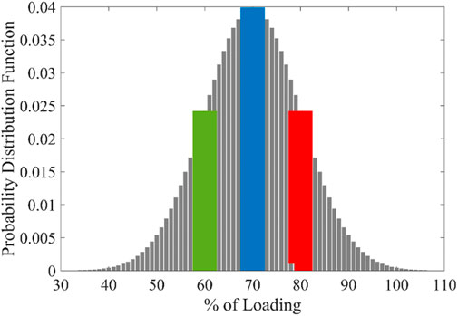
FIGURE 7. Gaussian distribution function for the generation of scenarios.

Where $P_{di}^{low}$ and $P_{di}^{high}$ are the low and high levels of ith scenario. Now, the mean of the ith level of loading $\overline{P_{d,i}}$:

$\overline{P_{d,i}}=\frac{1}{{\Delta }_{sc,i}}{\int }_{P_{di}^{low}}^{P_{di}^{high}}\left(P_d\times \frac{1}{{\sigma }_d\sqrt{2\pi }}{\mathrm{e}}^{\left[-\frac{{\left(P_d-{\mu }_d\right)}^2}{2{\sigma }_{d^2}}\right]}\right)d{P}_d(49)$

Table 5 contains the computer means and probabilities for all loading scenarios. After the creation of load scenarios and wind generation probabilities (as given in Section 3), these scenarios are then combined into a larger-scale master problem, where each scenario’s objective functions and constraints are treated as separate islands in a stacked network. Solving the MOOPF problem with a single solution for all scenarios when dealing with wind and probabilistic load models can offer several advantages.

TABLE 5

TABLE 5. Scenario-based variable load demand and its probability.

The master OPF problem enables greater flexibility in managing power systems since it provides uniformly distributed and wide final nondominated solutions for all scenarios that can be used to make real-time decisions. In each scenario, the proposed algorithm optimizes the power scheduled from all generators and also optimizes the locations of FACTS devices. The algorithm optimizes the locations of FACTS devices for all load levels. The program also adjusts each device’s ratings for the network’s various degrees of load. This study is useful because it uses MOOPF to run at predetermined intervals to optimize many, competing multi-objectives of an electrical network. Table 4 gives the constant minimum and maximum values for the decision vector under regulation. The outcomes of each simulation, which took into account the stochastic cost of energy generation and variable load demand, are shown in Table 6. It is evident from the decision variables shown in Table 6 that the BCS solution parameters are within the desirable range. The proposed algorithm was tested on three different cases with different objective functions.

TABLE 6

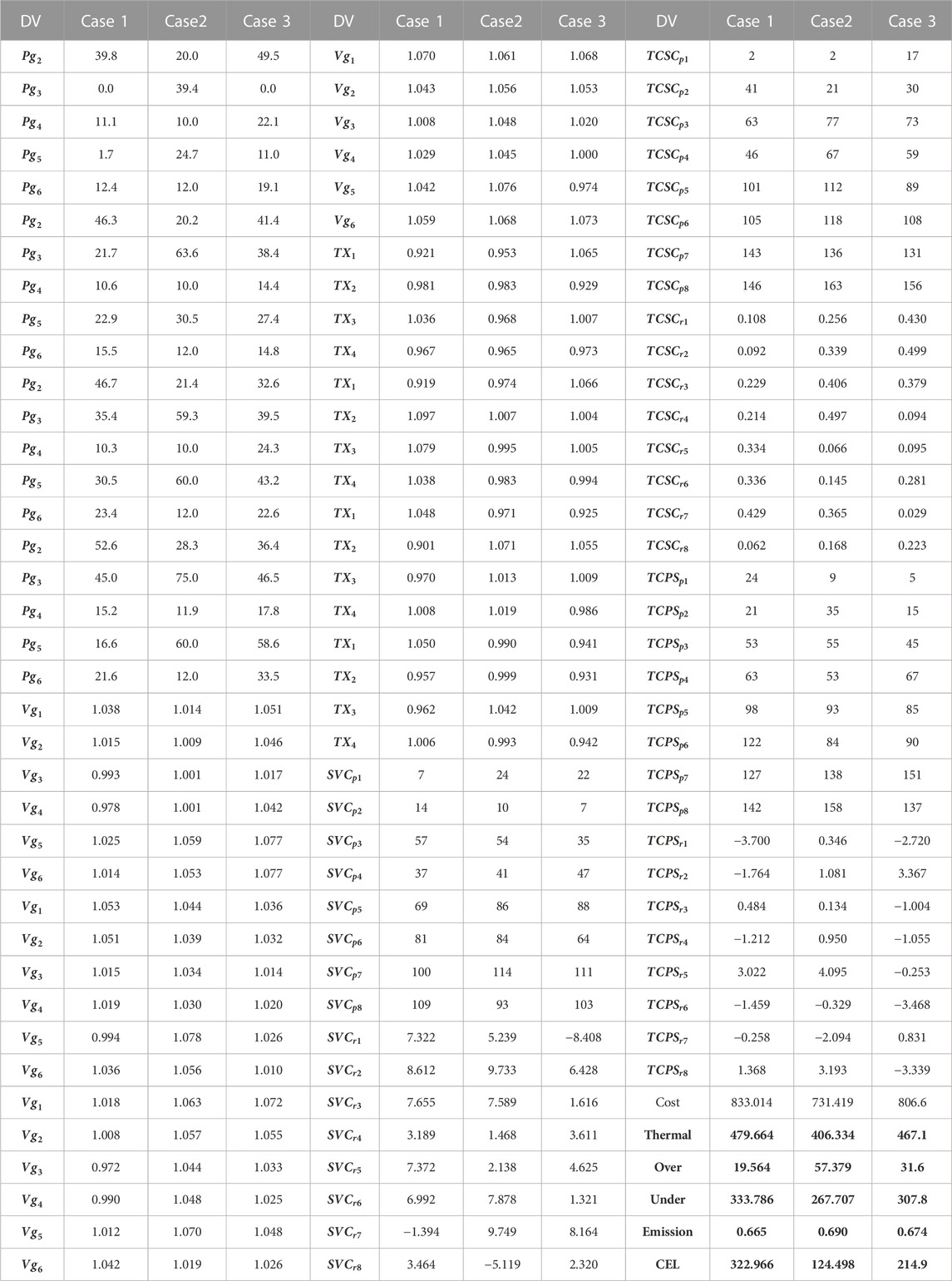
TABLE 6. Simulation results of various scenarios at different loading.

In Case 1, the algorithm achieved an expected cost of $833.014/h and an emission rate of conventional thermal generators of 0.665 t/h. In Case 2, the algorithm obtained a minimum cost of $731.419/h for active power generation and a cost of power loss is 124.498 $/h for energy loss. In Case 3, three objective functions were simultaneously minimized, resulting in costs of $806.6/h, 0.647 t/h for emissions, and $214.9/h for the cost of power loss.

Each case’s ideal FACTS device placement and size were identified, and they are shown in Table 6. For a particular situation that had the highest likelihood of occurring, the devices were positioned optimally, and the same optimal placements were applied for the remaining possibilities. In most cases, the FACTS devices operated near their peak values in scenario 4, where there was a large inductive load in the network. Optimizing the placement and rating of these devices can improve the efficiency, reliability, and cost-effectiveness of power systems. By analyzing the three cases, it became evident that the generation cost and cost of power loss were greater in Case 1. Tables 4, 6 show that in a realistic loading scenario, the cost of network operation and power loss are much reduced. Additionally, FACTS devices significantly modify their compensation in each case. The bar chart in Figure 8 shows the breakdown of a number of costs, such as the total cost of active power generation, the cost of thermal generators, the reserve and penalty cost of wind generators, and the cost of active power across the transmission line. The various elements that affect the price of wind energy and power losses in various scenarios are shown in Figure 8. First off, a low coefficient for the penalty function results in minor penalty costs in all scenarios. In Cases 2 and 3 of Scenario 4, running generators linked to Buses 5, 8, and 11 close to their maximum rated capacities can aid in minimizing power losses brought on by heavy network loading in those regions. But in Cases 1 and 3, underestimating wind energy might result in higher reserve costs due to direct, reserve, and penalty expenses for wind power. Due to lower scheduled power relative to Case 1, Cases 2 and 3’s thermal generator costs are lower. Consideration of power loss as an optimization aim can help to lower the cost of power loss, which is estimated based on the unit cost of energy. Figure 9 displays the BSC and final predicted nondominated solutions for each instance. Figure 9 show PF and the minimum values of the objective function, and the red color highlights the best compromise solution. Table 7 shows the state variables such as active power generated by slack bus generators and reactive power generated by all the PV bus generators of all the scenarios.

FIGURE 8

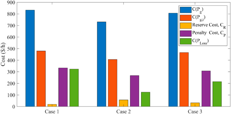
FIGURE 8. Comparison of Various costs for all the cases.

FIGURE 9

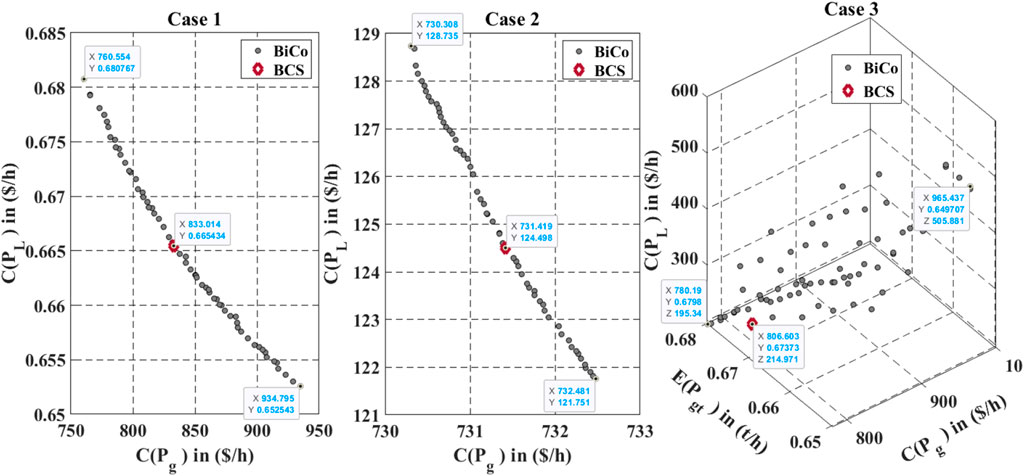
FIGURE 9. Best PF of BiCo of expected final nondominated solutions.

TABLE 7

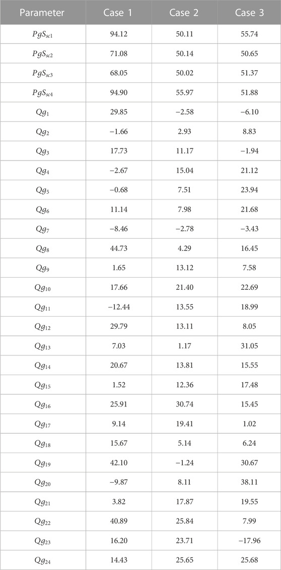
TABLE 7. Slack bus active and reactive power of all generators of all scenarios.

Table 7 shows that in Case 1, there is a wide range of possible values for the active MW injection at the slack bus. However, in Cases 2 and 3, the power generated by the slack bus generator is nearly equal across all scenarios. The bar charts in Figure 10 compare the active and reactive injections of all scenarios from the slack bus and PV bus generators respectively. Figure 10 also displays the load bus voltage profile for all scenarios. As can be seen in Figure 10, the voltage profiles on the load buses are well within the allowed range. In Case 1, the network voltage profile is very close to unity, however in Cases 2 and 3, the objective function includes the cost of active loss, which improves the voltage profile.

FIGURE 10

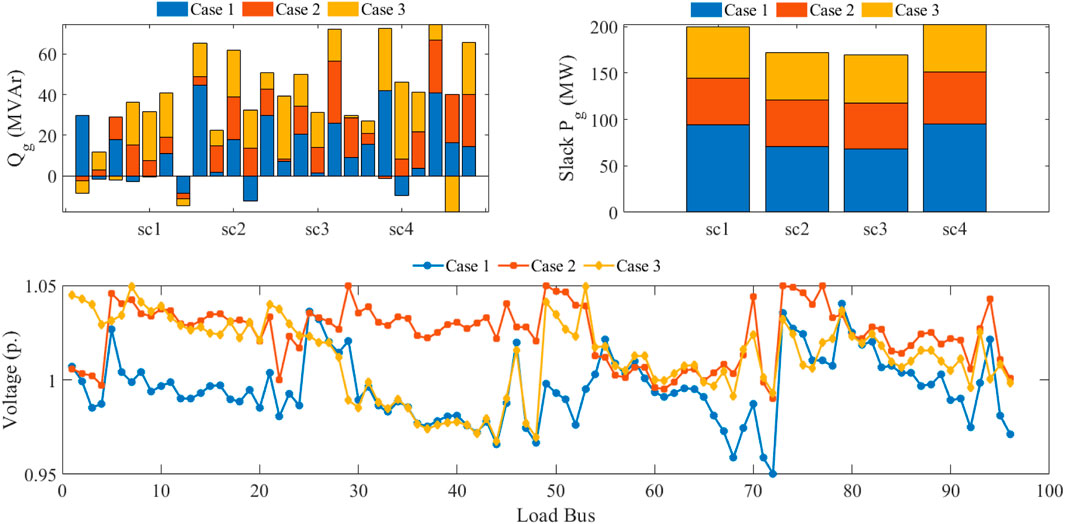
FIGURE 10. The state variables and voltage profiles for all the cases and events are shown in a bar chart.

6 Discussion

The main focus of this paper is on addressing the global need to reduce the carbon footprint and emissions by transitioning from fossil fuels to renewable energy sources for electricity generation. The study highlights the increasing complexity of the Multi-Objective Optimal Power Flow (MOOPF) problem, especially with the introduction of power electronics-based Flexible AC Transmission Systems (FACTS) devices. These FACTS devices offer a range of benefits, including improved controllability, effectiveness, stability, and sustainability in power systems. However, they also introduce uncertainty and variability, making the resolution of MOOPF issues challenging.

To address this, the paper develops three distinct cases with competing objective functions to find the optimal combination of control and state variables for MOOPF problems. These cases consider minimizing the total power generation cost, estimating the cost of wind generation, emission rate, and power loss due to transmission lines. The study covers both fixed and variable load scenarios. The proposed algorithm is put to the test in three different cases, yielding results that highlight its effectiveness. In Case 1, the algorithm achieved an expected cost of $833.014/h and an emission rate of 0.665 t/h for conventional thermal generators. In Case 2, it obtained a minimum cost of $731.419/h for active power generation and a cost of $124.498/h for energy loss. In Case 3, all three objective functions were minimized simultaneously, resulting in costs of $806.6/h for emissions, 0.647 t/h for emission rates, and $214.9/h for power loss.

The research emphasizes the importance of optimizing power systems for sustainability and efficiency, given the current developments in the power sector, including deregulation, integration of renewable energy sources, aging infrastructure, demand variability, and environmental concerns. The integration of FACTS devices is crucial in addressing these challenges and ensuring the reliability, efficiency, and stability of the power grid. The study goes further to compare the proposed algorithm with other state-of-the-art multi-objective evolutionary algorithms, demonstrating the proposed algorithm’s efficiency in providing a diverse range of non-dominated solutions. It discusses the significance of multi-objective optimization in handling complex power systems, especially with the growing integration of renewable energy sources. The paper’s contribution is in its focus on integrating both site and size modeling of FACTS devices into MOOPF solutions, potentially leading to more effective power system optimization. Furthermore, this study also emphasizes that multi-objective optimization is crucial for addressing the evolving challenges in the power sector, reducing environmental impact, and helping utilities meet their environmental targets and carbon footprint reduction goals.

7 Conclusion

FACTS are to enhance the controllability, efficiency, stability, and sustainability of power systems. Alternatively, wind integration in power systems offers a range of benefits including diversification of energy sources, environmental benefits, cost savings, local economic benefits, and energy independence. The optimal site and size of FACTS devices along with wind generation adds another level of uncertainty and variability to the power system, making it a challenging area of research to find the optimal solution to MOOPF problems. Therefore, in this work, the stochastic MOOPF problem with allocation and siting of FACTS devices and wind integration is modeled. The main objective of this study is to identify the best Pareto front of no-dominated solutions that satisfy all of the MOOPF problem’s operational and physical constraints while incorporating stochastic wind generation and the three types of FACTS devices that are most frequently used. Three study cases of conflicting objective functions such as minimization of the total cost of power produced, emission, and cost of energy loss produced by transmission line are formulated to find the optimal set of control and state variables of the MOOPF problem. The case studies involve conducting optimization analyses for power systems under both fixed and uncertain load demands. Appropriate probability density functions (PDFs) have been employed to model the random nature of both the wind energy and load demand to create representative scenarios of low and high probability. After that, all the scenarios are combined into the largescale master problem, whereas, objective functions and constraints of each scenario are treated as separate islands in a single stacked network. Simulation results show that the use of a single set of decision variables for all the scenarios is providing better trade between the conflicting objective functions and has advantages such as reduced computation time, improved accuracy, enhanced flexibility, improved system planning, and reduced risk. The cost of thermal generation, the direct cost of scheduled wind power, penalty charges for underestimating wind power, and reserve costs for overestimating wind power are all included in the total cost of the power supplied. Most recent multi-objective evolutionary algorithms are implemented analyzed and compared with the proposed algorithm. Simulation results show that the proposed algorithm finds the near global Pareto Front (PF) compared to the other MOEAs in most of the cases.

Data availability statement

The original contributions presented in the study are included in the article/supplementary material, further inquiries can be directed to the corresponding author.

Author contributions

AH: Formal Analysis, Writing–review and editing. AA: Conceptualization, Investigation, Writing–original draft, Writing–review and editing. MUK: Supervision, Writing–review and editing. NM: Formal Analysis, Writing–review and editing. GA: Conceptualization, Formal Analysis, Writing–original draft, Writing–review and editing. AK: Data curation, Software, Supervision, Writing–review and editing. SM: Validation, Writing–review and editing. AY: Project administration, Supervision, Validation, Visualization, Writing–original draft. ET: Software, Visualization, Writing–review and editing. MB: Funding acquisition, Validation, Writing–review and editing.

Acknowledgments

The authors declare financial support was received for the research, authorship, and/or publication of this article. The authors disclosed receipt of the following financial support for the research, authorship, and/or publication of this article: This work was funded by the Deanship of Scientific Research, King Faisal University Project No. “GRANT4778”.

Conflict of interest

The authors declare that the research was conducted in the absence of any commercial or financial relationships that could be construed as a potential conflict of interest.

Publisher’s note

All claims expressed in this article are solely those of the authors and do not necessarily represent those of their affiliated organizations, or those of the publisher, the editors and the reviewers. Any product that may be evaluated in this article, or claim that may be made by its manufacturer, is not guaranteed or endorsed by the publisher.

References

Abaci, K., and Yamacli, V. (2016). Differential search algorithm for solving multi-objective optimal power flow problem. Int. J. Electr. Power & Energy Syst. 79, 1–10. 2016/07/01/. doi:10.1016/j.ijepes.2015.12.021

CrossRef Full Text | Google Scholar

Abbas, G., Ali, B., Chandni, K., Koondhar, M. A., Chandio, S., and Mirsaeidi, S. (2022). A parametric approach to compare the wind potential of sanghar and gwadar wind sites. IEEE Access 10, 110889–110904. doi:10.1109/ACCESS.2022.3215261

CrossRef Full Text | Google Scholar

Abdo, M., Kamel, S., Ebeed, M., Yu, J., and Jurado, F. (2018). Solving non-smooth optimal power flow problems using a developed grey wolf optimizer. Energies 11 (7), 1692. doi:10.3390/en11071692

CrossRef Full Text | Google Scholar

Agrawal, R., Bharadwaj, S. K., and Kothari, D. P. (2018). Population based evolutionary optimization techniques for optimal allocation and sizing of Thyristor Controlled Series Capacitor. J. Electr. Syst. Inf. Technol. 5 (3), 484–501. 2018/12/01/. doi:10.1016/j.jesit.2017.04.004

CrossRef Full Text | Google Scholar

Ali, A., Abbas, G., Keerio, M. U., Koondhar, M. A., Chandni, K., and Mirsaeidi, S. (2023a). Solution of Constrained mixed-integer multi-objective optimal power flow problem considering the hybrid multi-objective evolutionary algorithm. IET Gener. Transm. Distrib. 17, 66–90. doi:10.1049/gtd2.12664

CrossRef Full Text | Google Scholar

Ali, A., Abbas, G., Keerio, M. U., Mirsaeidi, S., Alshahr, S., and Alshahir, A. (2023c). Pareto front-based multiobjective optimization of distributed generation considering the effect of voltage-dependent nonlinear load models. IEEE Access 11, 12195–12217. doi:10.1109/ACCESS.2023.3242546

CrossRef Full Text | Google Scholar

Ali, A., Abbas, G., Keerio, M. U., Mirsaeidi, S., Alshahr, S., and Alshahir, A. (2023d). Multi-objective optimal siting and sizing of distributed generators and shunt capacitors considering the effect of voltage-dependent nonlinear load models. IEEE Access 11, 21465–21487. doi:10.1109/ACCESS.2023.3250760

CrossRef Full Text | Google Scholar

Ali, A., Abbas, G., Keerio, M. U., Touti, E., Ahmed, Z., Alsalman, O., et al. (2023b). A Bi-level techno-economic optimal reactive power dispatch considering wind and solar power integration. Ieee Access 11, 62799–62819. doi:10.1109/ACCESS.2023.3286930

CrossRef Full Text | Google Scholar

Ali, B., Abbas, G., Memon, A., Mirsaeidi, S., Koondhar, M. A., Chandio, S., et al. (2023e). A comparative study to analyze wind potential of different wind corridors. Energy Rep. 9, 1157–1170. doi:10.1016/j.egyr.2022.12.048

CrossRef Full Text | Google Scholar

Basu, M. (2008). Optimal power flow with FACTS devices using differential evolution. Int. J. Electr. Power & Energy Syst. 30 (2), 150–156. 2008/02/01/. doi:10.1016/j.ijepes.2007.06.011

CrossRef Full Text | Google Scholar

Benabid, R., Boudour, M., and Abido, M. A. (2009). Optimal location and setting of SVC and TCSC devices using non-dominated sorting particle swarm optimization. Electr. Power Syst. Res. 79 (12), 1668–1677. 2009/12/01/. doi:10.1016/j.epsr.2009.07.004

CrossRef Full Text | Google Scholar

Berrouk, F., and Bounaya, K. (2018). Optimal power flow for multi-FACTS power system using hybrid PSO-PS algorithms. J. Control, Automation Electr. Syst. 29 (2), 177–191. 2018/04/01. doi:10.1007/s40313-017-0362-7

CrossRef Full Text | Google Scholar

Bhowmik, A. R., and Chakraborty, A. K. (2015). Solution of optimal power flow using non dominated sorting multi objective opposition based gravitational search algorithm. Int. J. Electr. Power & Energy Syst. 64, 1237–1250. 2015/01/01/. doi:10.1016/j.ijepes.2014.09.015

CrossRef Full Text | Google Scholar

Biswas, P., Arora, P., Mallipeddi, R., Suganthan, P., and Panigrahi, B. (2020). Optimal placement and sizing of FACTS devices for optimal power flow in a wind power integrated electrical network. Neural Comput. Appl. 33, 6753–6774. 11/05. doi:10.1007/s00521-020-05453-x

CrossRef Full Text | Google Scholar

Biswas, P. P., Suganthan, P., and Amaratunga, G. A. (2017). Optimal power flow solutions incorporating stochastic wind and solar power. Energy Convers. Manag. 148, 1194–1207. doi:10.1016/j.enconman.2017.06.071

CrossRef Full Text | Google Scholar

Biswas, P. P., Suganthan, P. N., Mallipeddi, R., and Amaratunga, G. A. J. (2018). Optimal power flow solutions using differential evolution algorithm integrated with effective constraint handling techniques. Eng. Appl. Artif. Intel. 68, 81–100. 2018/02/01/. doi:10.1016/j.engappai.2017.10.019

CrossRef Full Text | Google Scholar

Bouchekara, H. R. E. H., Chaib, A. E., Abido, M. A., and El-Sehiemy, R. A. (2016). Optimal power flow using an improved colliding bodies optimization algorithm. Appl. Soft Comput. 42, 119–131. 2016/05/01/. doi:10.1016/j.asoc.2016.01.041

CrossRef Full Text | Google Scholar

Chaib, A. E., Bouchekara, H. R. E. H., Mehasni, R., and Abido, M. A. (2016). Optimal power flow with emission and non-smooth cost functions using backtracking search optimization algorithm. Int. J. Electr. Power & Energy Syst. 81, 64–77. 2016/10/01/. doi:10.1016/j.ijepes.2016.02.004

CrossRef Full Text | Google Scholar

Chandrasekaran, S. (2020). Multiobjective optimal power flow using interior search algorithm: a case study on a real-time electrical network. Comput. Intell. 36 (3), 1078–1096. 2020/08/01. doi:10.1111/coin.12312

CrossRef Full Text | Google Scholar

Chen, G., Lu, Z., and Zhang, Z. (2018a). Improved krill herd algorithm with novel constraint handling method for solving optimal power flow problems. Energies 11 (1), 76. doi:10.3390/en11010076

CrossRef Full Text | Google Scholar

Chen, G., Qian, J., Zhang, Z., and Li, S. (2020). Application of modified pigeon-inspired optimization algorithm and constraint-objective sorting rule on multi-objective optimal power flow problem. Appl. Soft Comput. 92, 106321. 2020/07/01/. doi:10.1016/j.asoc.2020.106321

CrossRef Full Text | Google Scholar

Chen, G., Qian, J., Zhang, Z., and Sun, Z. (2019). Multi-objective optimal power flow based on hybrid firefly-bat algorithm and constraints- prior object-fuzzy sorting strategy. IEEE Access 7, 139726–139745. doi:10.1109/ACCESS.2019.2943480

CrossRef Full Text | Google Scholar

Chen, G., Yi, X., Zhang, Z., and Lei, H. (2018c). Solving the multi-objective optimal power flow problem using the multi-objective firefly algorithm with a constraints-prior pareto-domination approach. Energies 11 (12), 3438. doi:10.3390/en11123438

CrossRef Full Text | Google Scholar

Chen, G., Yi, X., Zhang, Z., and Wang, H. (2018b). Applications of multi-objective dimension-based firefly algorithm to optimize the power losses, emission, and cost in power systems. Appl. Soft Comput. 68, 322–342. 2018/07/01/. doi:10.1016/j.asoc.2018.04.006

CrossRef Full Text | Google Scholar

Deb, K., Pratap, A., Agarwal, S., and Meyarivan, T. (2002). A fast and elitist multiobjective genetic algorithm: NSGA-II. IEEE Trans. Evol. Comput. 6 (2), 182–197. doi:10.1109/4235.996017

CrossRef Full Text | Google Scholar

Duman, S., Li, J., wu, L., and Guvenc, U. (2020). Optimal power flow with stochastic wind power and FACTS devices: a modified hybrid PSOGSA with chaotic maps approach. Neural Comput. Appl. 32, 8463–8492. 06/01. doi:10.1007/s00521-019-04338-y

CrossRef Full Text | Google Scholar

Dutta, S., Paul, S., and Roy, P. K. (2018). Optimal allocation of SVC and TCSC using quasi-oppositional chemical reaction optimization for solving multi-objective ORPD problem. J. Electr. Syst. Inf. Technol. 5 (1), 83–98. 2018/05/01/. doi:10.1016/j.jesit.2016.12.007

CrossRef Full Text | Google Scholar

E. E.-E. 3.000 (2023). Welcome to wind-turbine-models.com. Available at: https://en.wind-turbine-models.com/(accessed on June 8, 2023).

Google Scholar

Ghasemi, M., Ghavidel, S., Ghanbarian, M. M., and Gitizadeh, M. (2015). Multi-objective optimal electric power planning in the power system using Gaussian bare-bones imperialist competitive algorithm. Inf. Sci. 294, 286–304. 2015/02/10/. doi:10.1016/j.ins.2014.09.051

CrossRef Full Text | Google Scholar

Ghasemi, M., Ghavidel, S., Ghanbarian, M. M., Massrur, H. R., and Gharibzadeh, M. (2014). Application of imperialist competitive algorithm with its modified techniques for multi-objective optimal power flow problem: a comparative study. Inf. Sci. 281, 225–247. 2014/10/10/. doi:10.1016/j.ins.2014.05.040

CrossRef Full Text | Google Scholar

Habib, S., Abbas, G., Jumani, T. A., Bhutto, A. A., Mirsaeidi, S., and Ahmed, E. M. (2022). Improved whale optimization algorithm for transient response, robustness, and stability enhancement of an automatic voltage regulator system. Energies 15, 5037. doi:10.3390/en15145037

CrossRef Full Text | Google Scholar

Kumar, A. R., and Premalatha, L. (2015). Optimal power flow for a deregulated power system using adaptive real coded biogeography-based optimization. Int. J. Electr. Power & Energy Syst. 73, 393–399. doi:10.1016/j.ijepes.2015.05.011

CrossRef Full Text | Google Scholar

Kumari, M. S., and Maheswarapu, S. (2010). Enhanced genetic algorithm based computation technique for multi-objective optimal power flow solution. Int. J. Electr. Power & Energy Syst. 32 (6), 736–742. 2010/07/01/. doi:10.1016/j.ijepes.2010.01.010

CrossRef Full Text | Google Scholar

Li, Z., Cao, Y., Dai, L. V., Yang, X., and Nguyen, T. T. (2019). Optimal power flow for transmission power networks using a novel metaheuristic algorithm. Energies 12 (22), 4310. doi:10.3390/en12224310

CrossRef Full Text | Google Scholar

Liu, Z., and Wang, Y. (2019). Handling constrained multiobjective optimization problems with constraints in both the decision and objective spaces. IEEE Trans. Evol. Comput. 23, 870–884. doi:10.1109/TEVC.2019.2894743

CrossRef Full Text | Google Scholar

Mahdad, B., and Srairi, K. (2016). Security constrained optimal power flow solution using new adaptive partitioning flower pollination algorithm. Appl. Soft Comput. 46, 501–522. 2016/09/01/. doi:10.1016/j.asoc.2016.05.027

CrossRef Full Text | Google Scholar

Mandal, B., and Kumar Roy, P. (2014). Multi-objective optimal power flow using quasi-oppositional teaching learning based optimization. Appl. Soft Comput. 21, 590–606. 2014/08/01/. doi:10.1016/j.asoc.2014.04.010

CrossRef Full Text | Google Scholar

Mirsaeidi, S., Devkota, S., Wang, X., Tzelepis, D., Abbas, G., Alshahir, A., et al. (2023). A review on optimization objectives for power system operation improvement using FACTS devices. Energies 16, 161. doi:10.3390/en16010161

CrossRef Full Text | Google Scholar

Mohamed, A.-A. A., Mohamed, Y. S., El-Gaafary, A. A. M., and Hemeida, A. M. (2017). Optimal power flow using moth swarm algorithm. Electr. Power Syst. Res. 142, 190–206. 2017/01/01/. doi:10.1016/j.epsr.2016.09.025

CrossRef Full Text | Google Scholar

Mohseni-Bonab, S. M., Rabiee, A., and Mohammadi-Ivatloo, B. (2016). Voltage stability constrained multi-objective optimal reactive power dispatch under load and wind power uncertainties: a stochastic approach. Renew. Energy 85, 598–609. 2016/01/01/. doi:10.1016/j.renene.2015.07.021

CrossRef Full Text | Google Scholar

Mukherjee, A., and Mukherjee, V. (2016). Chaotic krill herd algorithm for optimal reactive power dispatch considering FACTS devices. Appl. Soft Comput. 44, 163–190. 2016/07/01/. doi:10.1016/j.asoc.2016.03.008

CrossRef Full Text | Google Scholar

Naderi, E., Pourakbari-Kasmaei, M., and Abdi, H. (2019). An efficient particle swarm optimization algorithm to solve optimal power flow problem integrated with FACTS devices. Appl. Soft Comput. 80, 243–262. 2019/07/01/. doi:10.1016/j.asoc.2019.04.012

CrossRef Full Text | Google Scholar

Niknam, T., Narimani, M. r., Jabbari, M., and Malekpour, A. R. (2011). A modified shuffle frog leaping algorithm for multi-objective optimal power flow. Energy 36 (11), 6420–6432. 2011/11/01/. doi:10.1016/j.energy.2011.09.027

CrossRef Full Text | Google Scholar

Niu, M., Wan, C., and Xu, Z. (2014). A review on applications of heuristic optimization algorithms for optimal power flow in modern power systems. J. Mod. Power Syst. Clean Energy 2 (4), 289–297. doi:10.1007/s40565-014-0089-4

CrossRef Full Text | Google Scholar

Ongsakul, W., and Bhasaputra, P. (2002). Optimal power flow with FACTS devices by hybrid TS/SA approach. Int. J. Electr. Power & Energy Syst. 24 (10), 851–857. 2002/12/01/. doi:10.1016/S0142-0615(02)00006-6

CrossRef Full Text | Google Scholar

Panda, A., and Tripathy, M. (2014). Optimal power flow solution of wind integrated power system using modified bacteria foraging algorithm. Int. J. Electr. Power & Energy Syst. 54, 306–314. 2014/01/01/. doi:10.1016/j.ijepes.2013.07.018

CrossRef Full Text | Google Scholar

Premkumar, M., Jangir, P., Sowmya, R., and Elavarasan, R. M. (2021). Many-objective gradient-based optimizer to solve optimal power flow problems: analysis and validations. Eng. Appl. Artif. Intel. 106, 104479. 2021/11/01/. doi:10.1016/j.engappai.2021.104479

CrossRef Full Text | Google Scholar

Pulluri, H., Naresh, R., and Sharma, V. (2017). An enhanced self-adaptive differential evolution based solution methodology for multiobjective optimal power flow. Appl. Soft Comput. 54, 229–245. 2017/05/01/. doi:10.1016/j.asoc.2017.01.030

CrossRef Full Text | Google Scholar

Rahmani, S., and Amjady, N. (2018). Improved normalised normal constraint method to solve multi-objective optimal power flow problem. IET Generation, Transm. Distribution 12 (4), 859–872. 2018/02/01. doi:10.1049/iet-gtd.2017.0289

CrossRef Full Text | Google Scholar

Roy, R., and Jadhav, H. T. (2015). Optimal power flow solution of power system incorporating stochastic wind power using Gbest guided artificial bee colony algorithm. Int. J. Electr. Power & Energy Syst. 64, 562–578. (in English). doi:10.1016/j.ijepes.2014.07.010

CrossRef Full Text | Google Scholar

Sebaa, K., Bouhedda, M., Tlemcani, A., and Henini, N. (2014). Location and tuning of TCPSTs and SVCs based on optimal power flow and an improved cross-entropy approach. Int. J. Electr. Power & Energy Syst. 54, 536–545. doi:10.1016/j.ijepes.2013.08.002

CrossRef Full Text | Google Scholar

Shabanpour-Haghighi, A., Seifi, A. R., and Niknam, T. (2014). A modified teaching–learning based optimization for multi-objective optimal power flow problem. Energy Convers. Manag. 77, 597–607. 2014/01/01/. doi:10.1016/j.enconman.2013.09.028

CrossRef Full Text | Google Scholar

Shafik, M. B., Chen, H., Rashed, G. I., and El-Sehiemy, R. A. (2019). Adaptive multi objective Parallel seeker optimization algorithm for incorporating TCSC devices into optimal power flow framework. IEEE Access 7, 36934–36947. doi:10.1109/ACCESS.2019.2905266

CrossRef Full Text | Google Scholar

Shaheen, A. M., Farrag, S. M., and El-Sehiemy, R. A. (2016). MOPF solution methodology. IET Generation, Transm. Distribution 11 (2), 570–581. 2017/01/01 2017. doi:10.1049/iet-gtd.2016.1379

CrossRef Full Text | Google Scholar

Shehata, A. A., Tolba, M. A., El-Rifaie, A. M., and Korovkin, N. V. (2022). Power system operation enhancement using a new hybrid methodology for optimal allocation of FACTS devices. Energy Rep. 8, 217–238. 2022/11/01/. doi:10.1016/j.egyr.2021.11.241

CrossRef Full Text | Google Scholar

Shi, L. B., Wang, C., Yao, L. Z., Ni, Y. X., and Bazargan, M. (2012). Optimal power flow solution incorporating wind power. Ieee Syst. J. 6 (2), 233–241. (in English). doi:10.1109/Jsyst.2011.2162896

CrossRef Full Text | Google Scholar

Skolfield, J. K., and Escobedo, A. R. (2022). Operations research in optimal power flow: a guide to recent and emerging methodologies and applications. Eur. J. Oper. Res. 300 (2), 387–404. 2022/07/16/. doi:10.1016/j.ejor.2021.10.003

CrossRef Full Text | Google Scholar

Sun, R., Zou, J., Liu, Y., Yang, S., and Zheng, J. (2022). A multi-stage algorithm for solving multi-objective optimization problems with multi-constraints. IEEE Trans. Evol. Comput. 27, 1207–1219. doi:10.1109/TEVC.2022.3224600

CrossRef Full Text | Google Scholar

Tian, Y., Zhang, T., Xiao, J., Zhang, X., and Jin, Y. (2020). A coevolutionary framework for constrained multiobjective optimization problems. IEEE Trans. Evol. Comput. 25 (1), 102–116. doi:10.1109/tevc.2020.3004012

CrossRef Full Text | Google Scholar

Trivedi, I. N., Jangir, P., Parmar, S. A., and Jangir, N. (2018). Optimal power flow with voltage stability improvement and loss reduction in power system using Moth-Flame Optimizer. Neural Comput. Appl. 30 (6), 1889–1904. 2018/09/01. doi:10.1007/s00521-016-2794-6

CrossRef Full Text | Google Scholar

Varadarajan, M., and Swarup, K. S. (2008). Solving multi-objective optimal power flow using differential evolution. IET Generation, Transm. Distribution 2 (5), 720–730. doi:10.1049/iet-gtd:20070457

CrossRef Full Text | Google Scholar

Warid, W., Hizam, H., Mariun, N., and Abdul-Wahab, N. I. (2016). Optimal power flow using the Jaya algorithm. Energies 9 (9), 678. doi:10.3390/en9090678

CrossRef Full Text | Google Scholar

Wei, Y., Shuai, L., and Yu, D. C. (2004). A novel optimal reactive power dispatch method based on an improved hybrid evolutionary programming technique. IEEE Trans. Power Syst. 19 (2), 913–918. doi:10.1109/TPWRS.2004.826716

CrossRef Full Text | Google Scholar

Yuan, X., Zhang, B., Wang, P., Liang, J., Yuan, Y., Huang, Y., et al. (2017). Multi-objective optimal power flow based on improved strength Pareto evolutionary algorithm. Energy 122, 70–82. 2017/03/01/. doi:10.1016/j.energy.2017.01.071

CrossRef Full Text | Google Scholar

Zhang, J., Tang, Q., Li, P., Deng, D., and Chen, Y. (2016). A modified MOEA/D approach to the solution of multi-objective optimal power flow problem. Appl. Soft Comput. 47, 494–514. 2016/10/01/. doi:10.1016/j.asoc.2016.06.022

CrossRef Full Text | Google Scholar

Ziaee, O., and Choobineh, F. (2017a). Optimal location-allocation of TCSCs and transmission switch placement under high penetration of wind power. IEEE Trans. Power Syst. 32 (4), 3006–3014. doi:10.1109/TPWRS.2016.2628053

CrossRef Full Text | Google Scholar

Ziaee, O., and Choobineh, F. F. (2017b). Optimal location-allocation of TCSC devices on a transmission network. IEEE Trans. Power Syst. 32 (1), 94–102. doi:10.1109/TPWRS.2016.2556424

CrossRef Full Text | Google Scholar

Zimmerman, R. D., Murillo-Sanchez, C. E., and Thomas, R. J. (2009). “MATPOWER's extensible optimal power flow architecture,” in 2009 IEEE Power & Energy Society General Meeting, New York, USA, 26-30 July 2009, 1–7. doi:10.1109/PES.2009.5275967

CrossRef Full Text | Google Scholar

Zimmerman, R. D., Murillo-Sanchez, C. E., and Thomas, R. J. (2011). MATPOWER: steady-state operations, planning, and analysis tools for power systems research and education. IEEE Trans. Power Syst. 26 (1), 12–19. doi:10.1109/tpwrs.2010.2051168

CrossRef Full Text | Google Scholar