 Farwa Saeed1,2Abdul Ghafoor2Muhammad Imtiaz Hussain3
 Kamran Ikram1
 Muhammad Faheem2Muhammad Shahzad4
 Waseem Amjad4
 Muhammad Mubashar Omar4*Gwi Hyun Lee5*
- 1Department of Agricultural Engineering, Khawaja Fareed University of Engineering and Information Technology, Rahim Yar Khan, Pakistan
- 2Department of Farm Machinery and Power, Faculty of Agricultural Engineering and Technology, University of Agriculture Faisalabad, Faisalabad, Pakistan
- 3Agriculture and Life Sciences Research Institute, Kangwon National University, Chuncheon, Republic of Korea
- 4Department of Energy Systems Engineering Faculty of Agricultural Engineering and Technology, University of Agriculture Faisalabad, Faisalabad, Pakistan
- 5Interdisciplinary Program in Smart Agriculture, Kangwon National University, Chuncheon, Republic of Korea
Power generation from fossil fuels is the biggest challenge in the next half of the century. Alternative power generation techniques such as solar photovoltaic (PV) show potential to act as a future fuel with a challenge to efficiently convert the harvested solar energy into electrical power. This investigation conclusively focused on setting a 2.160-kW solar PV system capable of working at a higher efficiency by developing a mechanical structure that optimizes power production and minimizes energy losses. In addition to that, solar PV system efficiencies at various tracking positions, performance coefficients during rainy and sunny days, and system degradation rates have also been investigated. The PVsyst v6.8 simulation tool was used to obtain the simulated results, which were compared with the actual experimental results. The parameters considered for the investigations include ambient temperature, irradiance, solar PV module surface temperature, solar PV voltage and current, wind velocity, and atmospheric turbidity. The solar PV system was evaluated based on two modes, namely, M1 (no tracking/fixed type) and M2 (manual tracking by changing the position of the solar PV system every hour). The predictive results obtained using PVsyst v6.8 concluded that total energy production from the installed system was 3,242 kWh/yr and 3,984 kWh/yr for M1 and M2, respectively. The performance ratio (PR), obtained from simulation, was 72% and 78% for M1 and M2, respectively, which was consistent with the experimental results, i.e., 70% and 72% for M1 and M2, respectively. Similarly, the power conversion efficiencies under standard temperature and conditions for both modes, simulated and experimental, were found to be 16.50% and 12.75%, respectively. The estimated degradation rate was observed in the range of −0.6% to −5.0%.
Introduction
The US Energy Information Administration (EIA) predicts that by 2040, more than 10 trillion kilowatt hours of energy will be produced using renewable energy sources (Sawin et al., 2016). At present, Pakistan’s total electricity generation capacity from sunlight is 41.5 GW (NTDC, 2008), with 70% of its area receiving solar radiation in the range 5.0–5.5 kWh/m2/day (Harijan, 2008). The solar photovoltaic (PV) energy generation potential of a few renowned cities of Pakistan is shown in Table 1 below (ESMAP, 2021).

TABLE 1. Solar energy potential of different cities of Pakistan.
Solar PV modules provide an option to convert solar energy into electrical energy. These modules are usually mounted on the rooftop or at the available ground area. Energy conversion efficiency is always a major concern while installing any solar PV system. Three techniques are reported to increase the solar PV system efficiency, namely, 1) using a tracking system; 2) improving the efficiency of a power conversion algorithm; and 3) improving the power generation efficiency of the solar PV system (Muhammad et al., 2019). Studies on different tracking systems reported a 30%–60% increase in system power output (Serhan and Chaar, 2010; Otieno, 2015). Tracking is categorized into single-axis and double-axis tracking systems. The single-axis tracking system adjusts the azimuthal angle with a fixed altitude angle, whereas the double-axis tracking system adjusts the azimuthal and altitude angles. Several authors (Chang, 2009a; Chang, 2009b; Li et al., 2010; Li et al., 2011; Seme and Stumberger, 2011; Sallaberry et al., 2015) conducted studies on single-axis systems, while other scholars (Arbab et al., 2009; Eke and Sentruk, 2012; Song et al., 2013; Sun et al., 2017) conducted research on double-axis tracking systems. Huang et al. introduced a single-axis three-point solar PV module tracking system with three fixed angles for PV module movement in the morning, noon, and afternoon. The sun trackers were controlled by inducing a controller system. The comparative tests for fixed and three-point tracked PV systems concluded a 37.5% power increment via a single axis three-point manual tracking solar PV system (Huang et al., 2012; Chowdhury, 2019). A comparative study of single-axis solar PV tracking systems with fixed-mount modules using a bidirectional DC motor in a single-axis tracking system concluded 13% extra output power compared to a fixed-mount PV module system. Krishnan et al. (2021) and Caton (2014) studied single-axis and dual-axis tracking for a PV module system (used for water pumping) installed in a West African village. The proposed design of a single vertical axis at a fixed titled angle of 30° proved the best performance among all other techniques (Caton, 2014). Baykara compared the single-axis solar PV tracking system and stationary solar PV system. The output power generation was enhanced by 28.3% in terms of the single-axis tracking system compared with the static system (Baykara et al., 2020). Nageh et al. (2021) conducted a study on energy gain comparison between automatic and manual solar tracking systems and concluded that 8% more output power depends on the local site latitude and longitude. Ahmed et al. (2013) designed a low-cost solar PV tracking system and reported that the main problems in stand-alone tracking systems include high initial cost and high power consumption of the tracking system (Ahmad et al., 2013). Few researchers conducted studies on complex tracking systems, but these were not adopted because of their complex structure and mechanism. Automatic tracking systems require electronic and hydraulic components for solar PV module movement, which makes the system expensive (Abu-Khader et al., 2008; Sungur, 2009). These tracking systems consume high power to rotate PV modules, thus reducing the system's efficiency. Very few studies on solar tracking systems are reported in Pakistan. Mehdi et al. (2019) developed a single-axis solar tracking system and reported 1,742.88 Wh of energy from the installed optimized solar PV system compared with 829.6 Wh of energy from the same system with no tracking mechanism. Arham Hashmi et al. (2018) developed a gravity-based tracker for the Scheffler concentrator, which was utilized only for 6 h of cooking. Ali Memon et al. (2021) found an optimum tilt angle of 29.5o for a solar PV system installed at the Sukkur city of Pakistan. Kumar et al. (2019) conducted a case study for the performance evaluation of a 200-kW roof-integrated solar PV system based on the capacity factor, performance ratio (PR), and efficiency and estimated the system’s annual capacity factor (16.72%) and performance ratio of 77.27%. In reference to the literature cited, it was found that insufficient attention has been paid until now to developing a low-cost and efficient solar PV tracking system in the country. However, automatic systems are not suitable for small-scale energy production units due to their high price and complex mechanisms.
Therefore, the objective of this study was to develop a simple and low-cost manual solar PV module tracking system that enhances system power generation efficiency, along with a reduction in energy parasitic losses. Then, the performance evaluation of the solar PV systems based on the optimized structure capable of manual tracking was compared with the fixed-type solar PV system. The obtained results were also evaluated using numerical and empirical approaches via a simulation technique.
Materials and methods
Site description
Faisalabad city (31.42⁰ N, 73.083⁰ E), with an altitude of 190 m from the mean sea level, has a semi-arid climate with a mean annual rainfall of 0.615 m during the monsoon season (July and August) (Faheem et al., 2020). The average climatic conditions of the study area are given in Figure 1 and Figure 2.
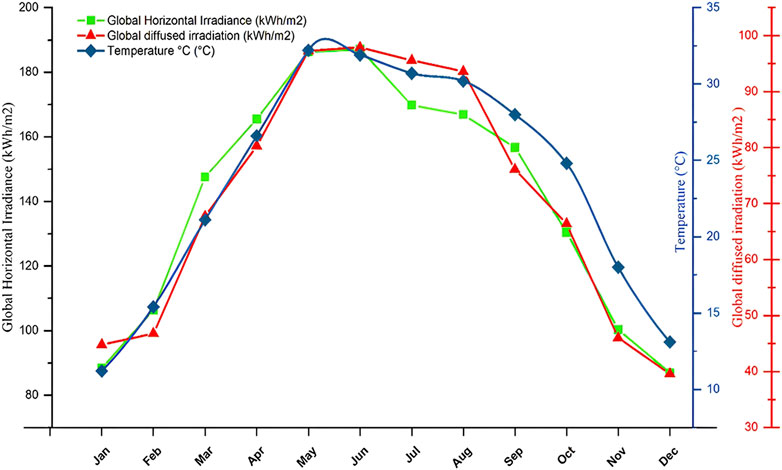
FIGURE 1. Average annual temperature variation and irradiation of the study area.
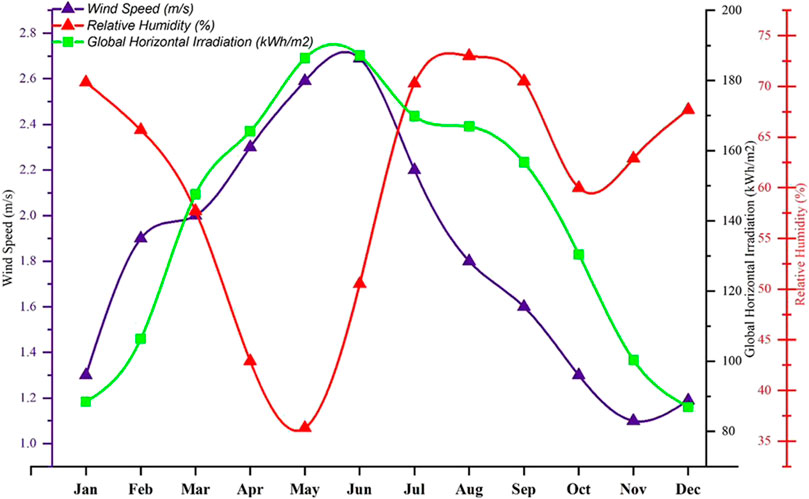
FIGURE 2. Average annual weather conditions of the study area.
Figure 1 shows an increase in temperature and solar irradiance from January to May–June, and then, it starts decreasing until it is minimal during December. Figure 2 supports Figure 1 as the relative humidity during May is the lowest with the highest temperature during this month.
Solar PV system description
A solar PV system with a rated capacity (2160 Wp) and one hybrid solar inverter were purchased from the local market in Faisalabad. The specifications of the solar PV modules and solar hybrid inverter are given in Table 2.
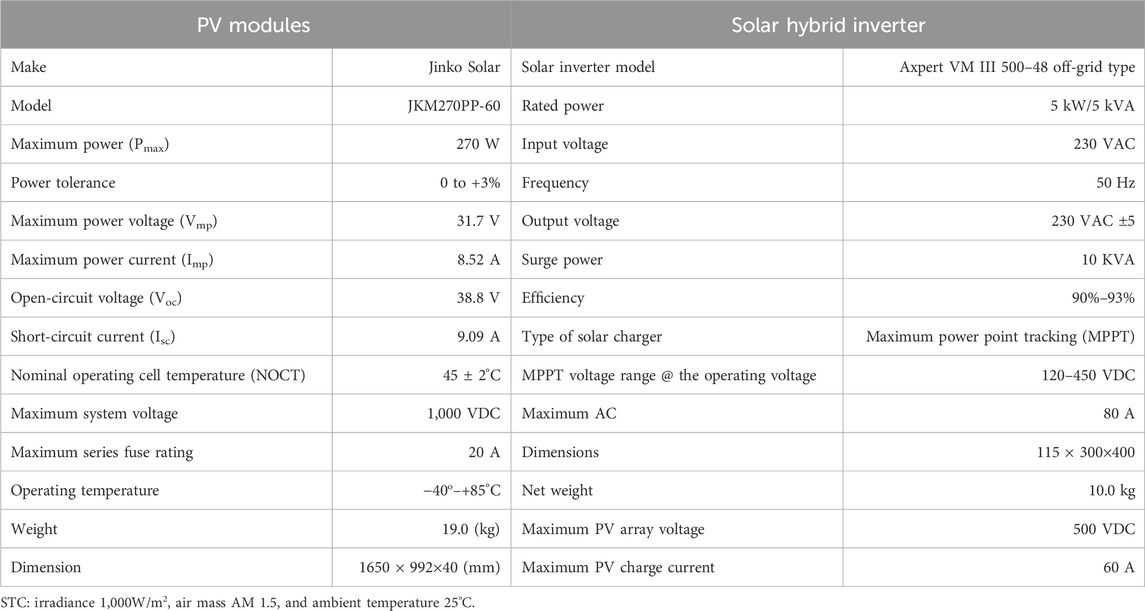
TABLE 2. Specifications of the installed solar PV modules and hybrid solar inverter.
Two frames were fabricated to install the PV modules at a shade-free location of the study area. The installed PV system comprised a hot-dipped galvanized iron pole with a vertical central pole with a baseplate, and side poles held with a T-frame—holding two adjustment angles for manual tracking into three different positions (Ghafoor et al., 2019). The PV array had eight solar PV modules in a single string, in which each module was made of 60 polycrystalline black silicon solar cells connected in series. The DC cables were attached to solar PV modules used for the transfer of total energy and were made of 99.9% copper, having a cross-section of 6 mm2 and a temperature range of −40°C–90°C.
Solar radiation measurements
The solar radiation intensity directly influences the power produced by the solar PV system. Solar irradiance is a measure of the rate of incident solar energy per unit area. Its value on a clear day is set as 1,000 Wm−2. Solar radiations above Earth’s atmosphere are called the solar constant. When these radiations enter the atmospheric territory, they are dispersed into diffused, reflected, and incident radiations. On a clear day, 85%–90% of the solar radiations are normally incident radiations (Ahmad et al., 2013). The incident radiations Id strike the solar PV surface and decrease with the increase in the incident angle θi. The relationship between the incident angle and incident radiation is obtained using Eq. 1:
Similarly, the data on the Sun position were also calculated to obtain the minimum incident angle for maximum energy production. Moreover, the experimental performance regarding data collection is shown in Annexure I at the end of the paper.
Sun position
To obtain the maximum energy from the installed PV system (using a manual solar tracking system), basic knowledge about the Sun position and angle is important for designing the tracking system. Two angles, the altitude angle (α) and azimuthal angle (γ), completely describe the solar position according to any location. The altitude angle was calculated using the data on the local altitude (φ), solar declination angle (δ), and local hour (ω), as given in Eq. 2 (Ahmad et al., 2013):
Similarly, the azimuthal angle was calculated using Eq. 3:
The solar declination was estimated using Eq. 4:
where n is the number of days in the year starting on 1 January as 1 and 31 December as 365.
The solar hour angle was taken as 15o as the Sun has to cover 360o in 24 h (Ullah et al., 2019). Simulation tools were used to describe the solar position during different months of the year. The Sun position data were used to design a manual tracking system that increases the power generation efficiency of the installed system. The zenith and azimuthal angles are shown in Figure 3.
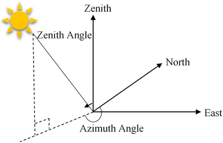
FIGURE 3. Azimuth and Zenith angles of a particular location with respect to sun.
Available solar radiations on a horizontal surface at any time of the day
The solar energy available in an area for a certain time interval is called solar radiation. The solar energy is calculated in Whm-2 or Jm-2. At any time, the apparent extraterrestrial radiation surface was calculated using Eq. 5 (Ahmad et al., 2013):
The value for Cosθz was calculated using Eq. 6:
Experimental procedure to analyze energy production from PV modules
The solar PV system performance was determined by comparing analytical and simulation methods. The experiments were conducted to estimate the power generation under different weather conditions on clear/bright, cloudy, and rainy days. The installed system was set facing the south to obtain maximum efficiency, whereas two solar tracking modes were chosen for this investigation.
1. Fixed tilted plane with no tracking system (M1).
2. Manual tracking system (M2).
In the fixed-mode type, the solar PV modules were set at fixed positions as undergoing a common practice in local areas, whereas, in a manual tracking system, the solar PV modules were rotated according to the change in the Sun position after every 1-h interval. After a day, the modules were set at their initial position in the evening to start tracking for the next day. Power production was estimated experimentally and through simulations between fixed (M1) and tracked (M2) modes of the installed PV array on a daily, monthly, and annual basis under local climatic conditions of the study area (Faisalabad city, Pakistan).
To calculate the power production from the solar PV system, data were collected in the following steps.
1. Data on the experimental site, PV system capacities, specifications, and mode of tracking.
2. Simulation study using PVsyst v6.88 to estimate the power production and type of losses in the system.
3. Energy performance and degradation rate.
4. PV system performance estimation using the methodology described by Kumar et al. (2019), as given in Table 3.
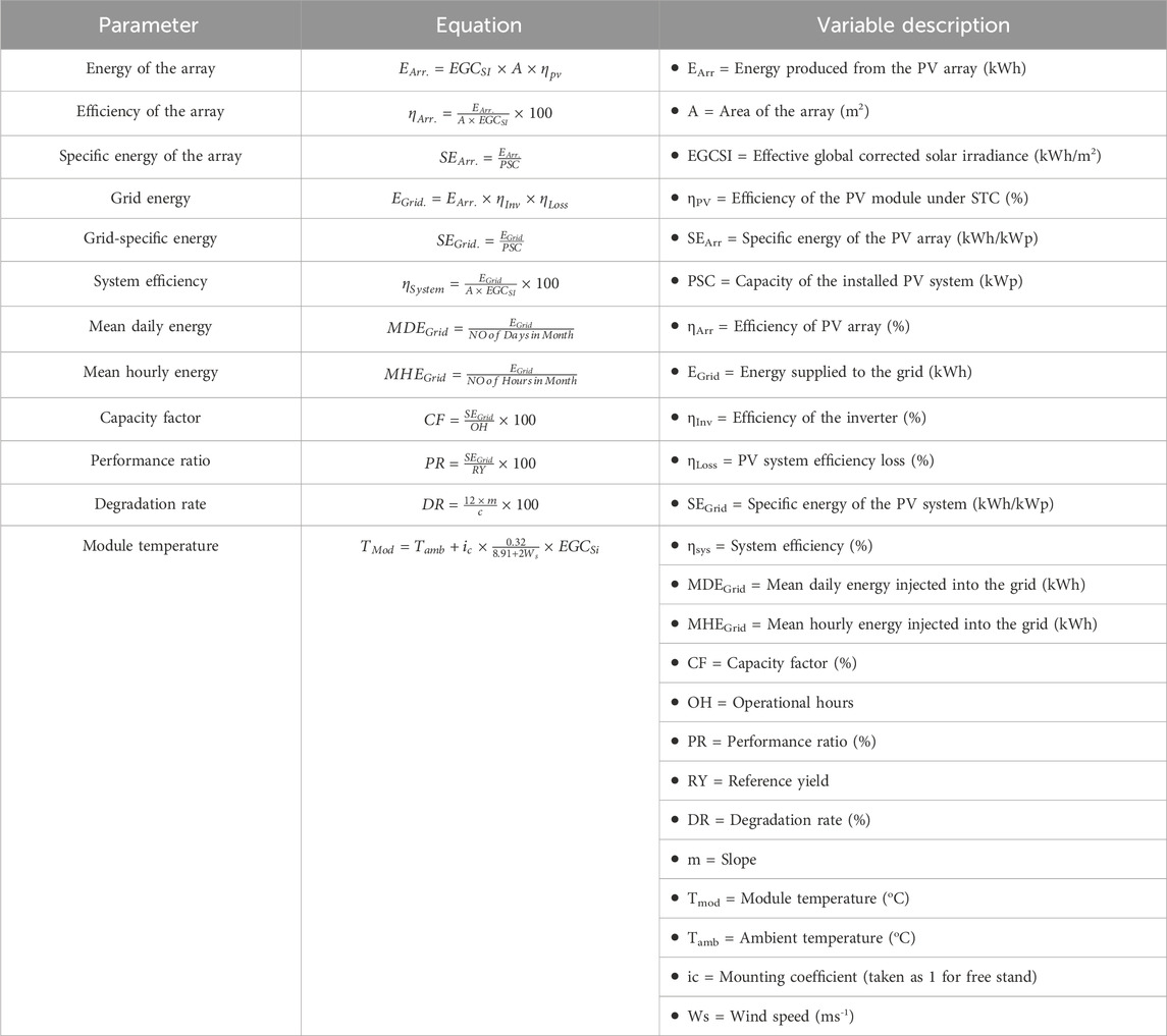
TABLE 3. Performance methodology described by Kumar et al. (2019).
PV system modeling procedure
Keeping in view the local climatic conditions, simulations of the installed system for power production and annual yield forecast were done using PVsyst v6.88. Input parameters included latitude, longitude, and coordinates of the study area, which were used for the determination of local climatic parameters such as the daily incoming solar radiation, wind speed, atmospheric temperature, and relative humidity. Similarly, the input parameters for PVsyst software, along with the Sun position need to be selected for the simulated study of the PV system model. Table 4 presents the specifications of input parameters for simulations of the study area. Figure 4 shows the mechanism for power generation for the solar PV system and various components used during this experimental investigation.
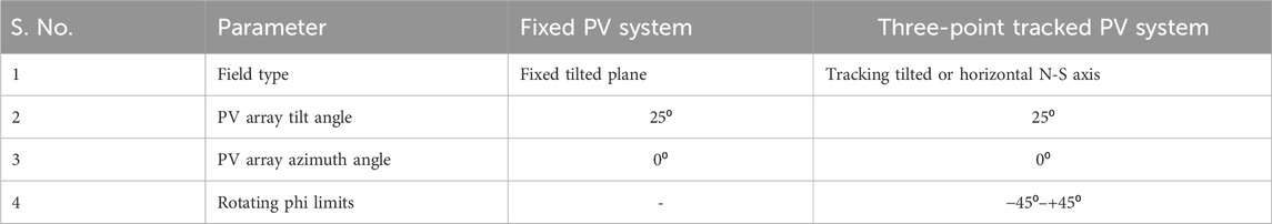
TABLE 4. PVsyst v6.88 computer simulation input parameters.
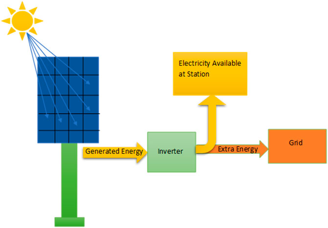
FIGURE 4. PV module system and components for power generation, as well as for the numerical and simulated study.
Instrumentations used for the investigation
Multiple instruments were used for data collection during the experiment, such as the bulb thermometer, silicon dome-type pyranometer, digital anemometer, digital probe thermometer, and digital clamp multimeter for the measurement of the ambient temperature, horizontal global irradiance, wind velocity, PV panel-surface temperature, DC voltage, and DC current, in addition to the overall array current and voltage separately (given in Table 5). The selected parameters were measured daily from 9:00 a.m. to 4:00 p.m. under different day conditions, viz., sunny, cloudy, heavy cloudy, and raining days for different months.
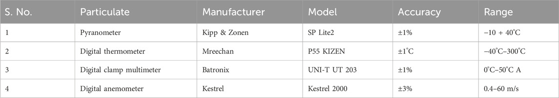
TABLE 5. Instrument specifications used for experimental data collection.
Simulation results
To conduct the energy balance of the PV system, computer-based simulations were performed for M1 and M2 conditions. The simulated results were found for average estimates of daily, monthly, and annual outcomes from 6:00 a.m. to 6:00 p.m. from January to December. Various other parameters like the produced energy, specific production, performance ratio, and system output power distribution plus the overall energy loss parameters were also considered.
Solar angle for the study area during different months of the year
The simulated Sun position shows the Sun angle throughout the year. Figure 5 shows the Sun height, and it was found to be the maximum for the summer season compared to spring, autumn, and winter seasons, respectively. As the month goes on from June to August, the Sun height starts to decline, as shown in Figure 5. Sun position-1 is the sun height for 22 June, at the 12th hour of the day length that is 80⁰ maximum for the given months. Sun position-4 indicates the equinox on 20 March and 23 September when day and night durations are equal. Position-5 specifies that the Sun position for the spring and fall seasons is 45⁰ sun height, and sun position-7 shows the sun height for 22 December, which is minimum at the 12th hour of a day course for a winter season that is only 35⁰. Here, 1 degree is equal to 111 km of distance in space as the sun rotates 1° in E-W and N-S. It means it covers 111 km of distance in the vertical/horizontal direction. Similarly, the location of the Sun in the study area based on hourly movements is shown in Table 6.
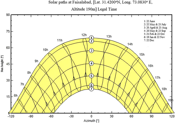
FIGURE 5. Simulated Sun path diagram from 6:00 a.m. to 6:00 p.m. in the study area.
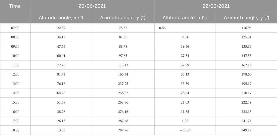
TABLE 6. Hourly sun location in the study area for 2 days.
Normalized production and performance ratio for M1 and M2
The normalized production for M1 and M2 revealed a combination of the losses such as 1) collection loss (Lc): the losses due to PV array found to be 0.77 kWh/kWp/day and 0.94 kWh/kWp/day, respectively; 2) system loss (Ls): the losses due to inverter operation were 0.24 kWh/kWp/day and 0.22 kWh/kWp/day, respectively; and 3) the produced useful energy inverter output loss (Yf) was 4.11 kWh/kWp/day and 5.0 kWh/kWp/day, respectively. The average annual PRs for M1 and M2 were observed to be 80.2% and 81.4%, respectively.
The graphical behavior of the normalized energy production and performance ratio of M1 and M2 from January to December is shown in Figure 6 and Figure 7, respectively. It was concluded that as the ambient temperature of the given site increases with every passing month, the performance ratio decreases month-wise due to the increase in temperature. The maximum performance ratio of 86.7% (M1) and 87.6% (M2) was noted in January, while the minimum performance ratio of 76.5% (M1) and 78.1% (M2) was noted in May.
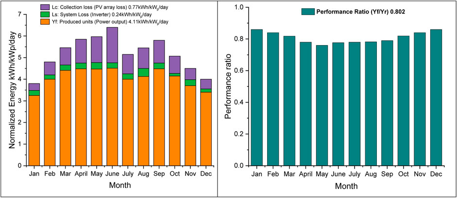
FIGURE 6. Normalized production and performance ratio of M1.
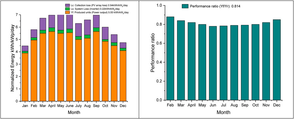
FIGURE 7. Normalized production and performance ratio of M2.
Daily input/output diagram for M1 and M2
The graphical results (Figure 8A for M1 and Figure 8B for M2) describe the daily input solar insolation in kWh/m2/day on the collecting plane from 6:00 a.m. to 6:00 p.m. and output-produced energy of the solar PV system in kWh/day. This shows a linear trend between input solar irradiance and output power production of a PV system. As the solar irradiance increases from morning to afternoon, the output power produced from the PV system also increases, as shown in Figures 8A,B. The peak incoming solar radiation amount was absorbed on the collecting plane from 12:00 to 3:00 p.m. in a day course, and more output energy was measured in that time interval for grid injection or public consumption.
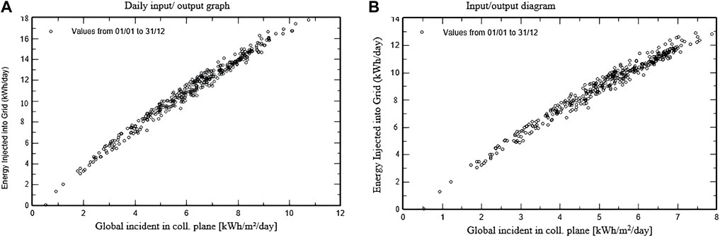
FIGURE 8. (A) represents Daily input-output for M1 and (B) represents Daily input-output for M2.
Figure 8A shows the daily input–output for M1, and Figure 8B represents the daily input–output for M2.
Energy loss diagram for M1 and M2
Figure 9 presents loss factors such as PV loss due to irradiance, temperature, module quality, ohmic wiring, inverter loss during operation, inverter loss over inverter nominal power, and inverter loss due to the power threshold. The energy loss diagram also shows that the horizontal global irradiation 1,692 kWh/m2 with effective irradiance on collectors was 1,816 kWh/m2 and 2,221 kWh/m2 for M1 and M2, respectively, and 3,924 kWh and 4,799 kWh as the array nominal energy (at STC efficiency) for M1 and M2, respectively. After some losses, only 3,432 kWh and 4,155 kWh were observed for the array virtual energy at MPP for M1 and M2, respectively, which resulted in available energy at the inverter output as 3,242 and 3,984 kWh for M1 and M2 over a year, respectively. The overall PV power conversion efficiency from DC to AC was found to be 16.50% for both modes of operation of the installed solar PV system.
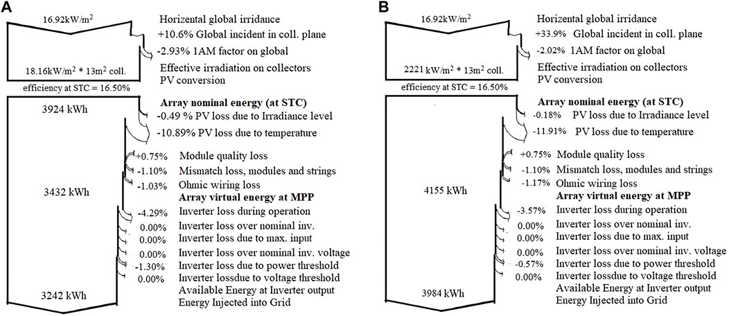
FIGURE 9. (A) Annual energy loss diagram for M1. (B) Annual energy loss diagram for M2.
Experimental results
The real-time data were collected from a single-axis three-point manually tracked solar PV system to analyze the working efficiency of research site conditions from 9:00 a.m. to 4:00 p.m. of M1 and M2 on different dates of February, March, June, and July. The important parameters to be considered for the investigation include solar irradiance, PV module surface temperature, site ambient temperature, PV array voltage and current, digital thermometer, bulb thermometer, and digital clamp multimeter to find the PV output power generation on a daily, weekly, monthly, and average annual estimation.
PV power production on a bright/luminous day
Real-time data were recorded continuously for 8 h from 9:00 a.m. to 16:00 p.m. (with a 1-h interval) on 9 March 2021, continuously tracking the Sun movement in a day course from morning to evening. It was noted that the solar PV system power output was observed to be higher from 9:00 a.m. to 01:00 p.m. as the PV array received more incoming irradiance from the Sun. The peak horizontal global radiations at 01:00 p.m. were recorded using the pyranometer on the panel surface, which was 904 W/m2, while an output power of 1,693 W was found in the tracked position (M2), and sun radiations of 880 W/m2 were measured on the same PV array, leading to a production of 1,605 W at a fixed position (M1). Afterward, from 02:00 p.m. to 04:00 p.m., a limited amount of solar radiation was received from the Sun. The total PV output energy after conversion from DC to AC was recorded at 11.412 kWh and 9.995 kWh in the cases of M2 and M1, respectively. Figure 10 presents the whole-day power production of the above PV system in both M1 and M2. The power conversion efficiency was calculated to be 11% on this sunny day.
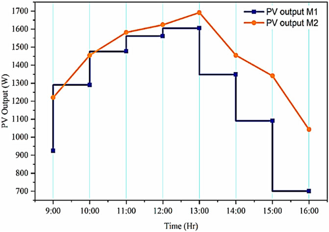
FIGURE 10. Real behavior of the PV system power generation on a luminous day.
PV power production on a cloudy day
The same experiment was conducted for the above-mentioned site and PV system modes M1 and M2 on 28 February 2021 for a cloudy day. Table 5 presents the estimated output power of the whole day, which is 5,640 W and 5,988 W for M1 and M2, respectively. The experimental data demonstrated that the presence of clouds caused a considerable irregular power production phenomenon such as at 11:00 a.m., 02:00 p.m., and 04:00 p.m. A minute amount of output power was generated because of the presence of dense clouds but no-rain condition, as shown in Figure 11, since the presence of clouds adversely affects the incident solar radiation amount.
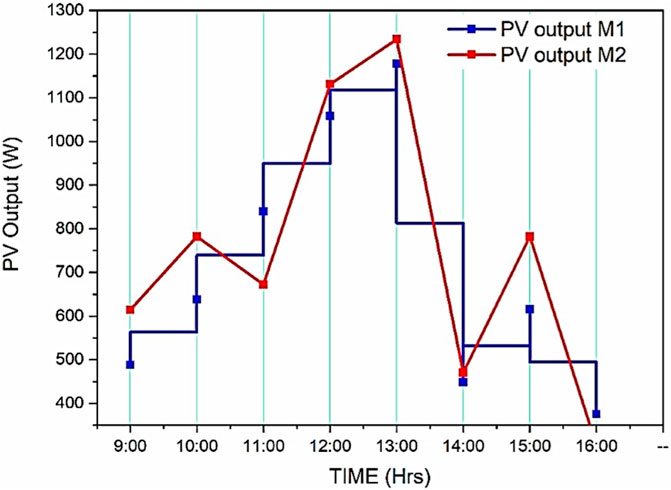
FIGURE 11. PV array power production behavior on a cloudy day.
The incident solar insolation and output power production were both relatively higher from 9:00 to 10:00 a.m. for M1 and M2. At 11:00 a.m., a sudden decrease in PV output power of M2 was observed, only 672 W, and an increase in power for M1 as 840 W was measured, as shown in Figure 12. From 12:00 p.m. to 01:00 p.m., the output power was magnified, and later on, at 02:00 p.m., the PV-produced output power was again escalated to 448 W and 470 W for M1 and M2, respectively. The total output energy was 5.640 kWh/day and 5.988 kWh/day of M1 and M2, respectively, along with only a PV array power conversion efficiency of 7.2%.
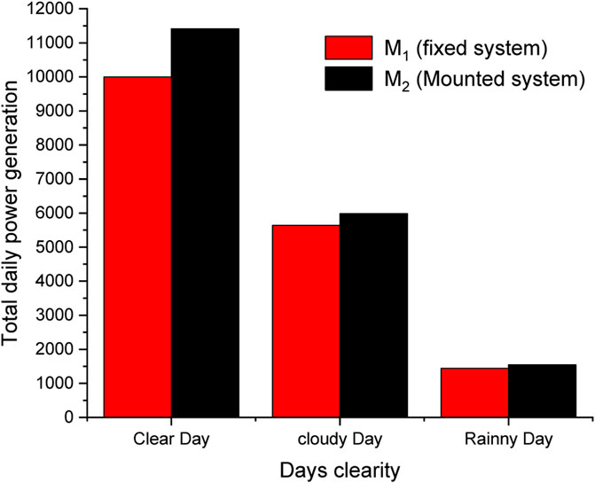
FIGURE 12. Comparison of power production under different weather conditions for the installed PV system.
PV power production on a rainy day
Real-time data were acquired to analyze the PV system performance on 11 March 2021 forecasted to have heavy clouds and rains. The experimental results of continuous 8 h found an abrupt decrease and increasing trend of power production, as shown in Figure 13. A negligible amount of PV output power was measured at 9:00 a.m. and 10:00 a.m. due to a heavy cloud cover in front of the Sun that prevented the sunlight from reaching the ground. At 11:00 a.m., zero power was recorded because of rain from the PV array. At 12:00 p.m., a significant quantity of power output was calculated from the measuring parameters.
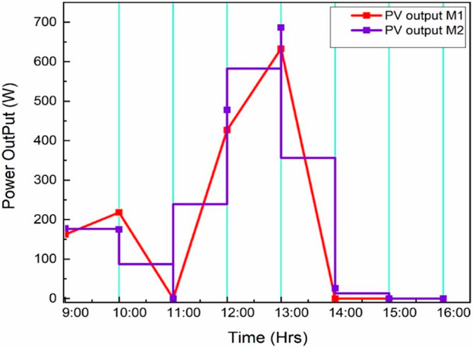
FIGURE 13. Power production of a PV system on a rainy day.
At 01:00 p.m., a peak power of 633 W and 687 W was produced for M1 and M2, respectively, in the presence of light clouds. Only 26 W of solar power was measured at 02:00 p.m., and no power was computed from the above PV system at 03:00 p.m. and 04:00 p.m. as a result of the full cloud cover along with the rains under local weather conditions of this study site. Table 6 presents the hourly power production from morning to evening, estimated to be 1.544 kWh and 1.440 kWh for M1 and M2, respectively, with a power conversion efficiency of 5.8%, as calculated from the measured data.
Performance ratio and power conversion efficiency for M1 and M2
During the experiment, the PR of the installed PV system was calculated in February, March, June, and July to be 72%, 75%, 71%, and 70% for M2, respectively, and 68%, 74%, 70%, and 69% for M1 of the array, respectively. The power conversion efficiency from real-time data was computed to be 11%, 12%, 19%, and 10% for both M1 and M2 in February, March, June, and July, respectively, using the method discussed by Harijan (2008). The simulation results estimated the PR in February, March, June, and July to be 85%, 82%, 78%, and 79% for M2 and 84%, 81%, 77%, and 78% for M1, respectively. The simulation results concluded an efficiency of 16.50% at STC and 12.75% from experimental results. The simulation results also collected an annual average energy of 3,242 kWh and 3,984 kWh obtained for M1 and M2, respectively, and the daily estimated energy to be 8.8 kWh/day and 10.8 kWh/day.
Degradation rate
There are many degradation modes that deteriorate the PV module performance like module delamination, hotspot failure, corrosion, glass breakage, and electro-migration in the contact layers, and interconnection, discoloration, and shading. These degradation modes affect the series and shunt resistance, and incoming solar radiation at the module surface. Hence, the study of the degradation mechanism is essential to ensure the reliability and long lifetime of PV modules. The degradation rate is difficult to calculate, and it requires substantial data (Dubey, 2016a). The degradation rate for the installed PV system at the investigation site was estimated to be −0.6% to −5%.
Discussion
The proposed study presented the performance evaluation of a single-axis three-point manual tracking and fixed solar system and compared the experimental results and computer-based simulated results for different parameters. Manual tracking, instead of automatic, was used in the system to keep it less complex. The total 8-PV panels were mounted on a single frame having three adjustment angles during morning, noon, and afternoon. A three-point manually tracked PV system was also introduced to reduce its initial installation and maintenance cost (Li et al., 2010).
The proposed study aimed to compare the experimental results of the system with the simulated results. PVsyst v6.8 was used to simulate the performance of the PV system. The simulated results displayed a detailed output-generated energy loss diagram that occurred during the operation of the PV system. The solar inverter directed electrical energy and converted DC to AC. Anjum (2018) reported that an increase in ambient temperature reduces the PV system efficiency and, hence, increases the losses. In the proposed study, the simulated result output reported that a significant amount of PV energy was lost with an increase in ambient temperature. Up to 11.91% and 10.89% of the energy in M2 and M1, respectively, was lost due to the excess ambient temperature of the present research site in the summer. Therefore, an increase in ambient temperature greatly affects the working quality of the PV module/array. Energy losses of 1.17% and 1.03% were found in DC cables and 3.57% and 4.29% through inverter operations for M2 and M1, respectively. It was also calculated that a power conversion efficiency of only 8% was obtained in July from the experimental results. Similar results were reported by Lavanya et al. (2018) by estimating PV system performance through the same simulation technique and reported that maximum power was generated during low-temperature months, and less energy production was predicted during high-temperature months. The operating nominal temperature range of the described PV module is 45°C ± 2°C, and the maximum temperature measured in July was 52°C at 13:00 p.m. Each 1°C increase in the PV module cell temperature from the STC conditions affects the same degree of deduction in the cell efficiency, as reported by Huang et al. (2012). Another parameter that contributes to the low absorption of irradiance by the collecting plane is the Linke turbidity (TL) coefficient. It is a combination of the water vapor content and aerosol present in the atmosphere that causes the absorbance and scattering of sun radiations and influences the PV system power production quality (Muhammad et al., 2019). Table 1 shows a measurable quantity of TL values for each month for the present study site. The degradation rate is essential to find the performance evaluation of a PV system. The predicted degradation rate of the installed PV system was −0.6 to −5. Dubey et al. (2016b), Dubey et al. (2017), and Kumar et al. (2019) reported the light-induced degradation and degradation rate. They further reported that this degradation depends on local climate and manufacturing factors. Previously reported studies predicted that the degradation rate for semi-arid climatic conditions was in the range 0.17%–0.30% (Kumar et al., 2019).
Conclusion
After carrying out the above study, it can be concluded that the above-mentioned PV system is a prime choice for electric energy production. Solar PV systems in the tracking mode contributed an average annual performance ratio of 80% and 81% for M1 and M2, respectively, via simulations and 70% and 72% for M1 and M2, respectively, via experimentation for the Faisalabad site under real climate conditions. Furthermore, an 18% increment in power production was reported using the manual tracking system, as against the fixed-PV system. The experimental results also justified that the presence of clouds and rains caused a major decrement in power production versus sunny days. Only a 34% PR was calculated for the rainy days of the tracked PV system and 32% for a fixed-PV system. The simulated results found an annual average energy generation of 3,242 kWh and 3,984 kWh for M1 and M2, respectively, suitable for domestic consumption or grid injection. This study focused on comparing the power production efficiency and energy losses of polycrystalline-type PV modules using a manual tracking system and simulation technique without considering the soiling effect. Future studies may be designed to compare the performance and energy losses in monocrystalline- and polycrystalline-type PV modules with manual- and automatic-type single- and double-axis tracking systems. This study may also include the soiling effect on the PV system power production efficiency.
Data availability statement
The original contributions presented in the study are included in the article/Supplementary Material; further inquiries can be directed to the corresponding authors.
Ethics statement
The studies involving humans were approved by the departmental committee of the University of Agriculture. The studies were conducted in accordance with the local legislation and institutional requirements. Written informed consent for participation was not required from the participants or the participants’ legal guardians/next of kin because they are far from the origin point now.
Author contributions
FS: formal analysis, data curation, and writing–original draft. AG: data curation, formal analysis, investigation, and writing–review and editing. MH: data curation, methodology, software, and writing–review and editing. KI: project administration, software, visualization, and writing–review and editing. MF: writing–review and editing. WA: methodology, project administration, and writing–review and editing. MO: formal analysis, supervision, visualization, and writing–review and editing. GL: formal analysis, funding acquisition, investigation, methodology, supervision, and writing–review and editing.
Funding
The author(s) declare financial support was received for the research, authorship, and/or publication of this article. This work was supported by the National Research Foundation of Korea (NRF) grant funded by the Korean government (MSIT) (No. 2022R1F1A1062793) and the Korea Institute of Planning and Evaluation for Technology in Food, Agriculture, and Forestry (IPET) through the Technology Commercialization Support Program, funded by the Ministry of Agriculture, Food and Rural Affairs (MAFRA) (No. 821048-3).
Conflict of interest
The authors declare that the research was conducted in the absence of any commercial or financial relationships that could be construed as a potential conflict of interest.
Publisher’s note
All claims expressed in this article are solely those of the authors and do not necessarily represent those of their affiliated organizations, or those of the publisher, the editors, and the reviewers. Any product that may be evaluated in this article, or claim that may be made by its manufacturer, is not guaranteed or endorsed by the publisher.
References
Abu-Khader, M. M., Badran, O. O., and Abdallah, S. (2008). Evaluating multi-axes sun-tracking system at different modes of operation in Jordan. Renew. Sustain Energy Rev. 12, 864–873. doi:10.1016/j.rser.2006.10.005
Ahmad, S., Shafie, S., and Mohd Zainal AbidinAhmad, A. K. N. S. (2013). On the effectiveness of time and date-based sun positioning solar collector in tropical climate: a case study in Northern Peninsular Malaysia. Renew. Sustain. Energy Rev. 28, 635–642. doi:10.1016/j.rser.2013.07.044
Ali Memon, Q., Rahimoon, A. Q., Ali, K., Fawad Shaikh, M., and Ahmed Shaikh, S. (2021). Determining optimum tilt angle for 1 MW photovoltaic system at Sukkur, Pakistan. Int. J. Photoenergy 2021, 1–8. doi:10.1155/2021/5552637
Anjum, S., and Beg, S. (2018). Design and performance Analysis of A grid connected solar photovoltaic system. IOSR J. Eng. (IOSRJEN) 08 (8), 06–10.
Arbab, H., Jazi, B., and Rezagholizadeh, M. (2009). A computer tracking system of solar dish with two-axis degree freedoms based on picture processing of bar shadow. Renew. Energy 34, 1114–1118. doi:10.1016/j.renene.2008.06.017
Arham Hashmi, S. A., Usman, M., Junaid, M., Badshah, S., and Nawaz, A. (2018). “Design & fabrication of gravity based solar tracker applied on scheffler reflector,” in 2018 International Conference on Power Generation Systems and Renewable Energy Technologies (PGSRET), Islamabad, Pakistan, 10th-12th September 2018, 1–4. doi:10.1109/PGSRET.2018.8686031
Baykara, Z. S., Figen, H. E., and karaismailoglu, M. (2020). “Environmental issues and social issues with renewable energy,” in Comprehensive renewable energy book. 2nd Edition.
Caton, P. (2014). Design of rural photovoltaic water pumping systems and the potential of manual array tracking for a west-african village. Sol. Energy 103, 288–302. doi:10.1016/j.solener.2014.02.024
Chang, T. P. (2009a). The gain of single-axis tracked panel according to extraterrestrial radiation. Appl. Energy 86 (7), 1074–1079. doi:10.1016/j.apenergy.2008.08.002
Chang, T. P. (2009b). Performance study on the east–west oriented single-axis tracked panel. Energy 34, 1530–1538. doi:10.1016/j.energy.2009.06.044
Chowdhury, M. E. H. (2019). Amith khandakar, belayat hossain, and rayaan abouhasera. A low-cost closed-loop solar tracking system based on the sun position algorithm. Hindawi J. Sensors 2019, 11. doi:10.1155/2019/3681031
Dubey, R. (2016a). An integrated framework of joint venture success. IJSBA 5, 1. doi:10.1504/IJSBA.2016.078248
Dubey, R., Chattopadhyay, S., Kuthanazhi, V., John, J., Ansari, F., Rambabu, S., et al. (2016b). O.S all-India survey of PV module reliability, 1–164.
Dubey, R., Chattopadhyay, S., Kuthanazhi, V., Kottantharayil,, A., Singh Solanki, C., Arora, B. M., et al. (2017). Comprehensive study of performance degradation of field-mounted photovoltaic modules in India. Energy Sci. Eng. 5, 51–64. doi:10.1002/ese3.150
Eke, R., and Sentruk, A. (2012). Performance comparison of a double-axis sun tracking versus fixed PV system. Sol. Energy 86, 2665–2672. doi:10.1016/j.solener.2012.06.006
Faheem, M., Jizhan, L., Akram, M. W., Khan, M. U., Yonphet, P., Tayyab, M., et al. (2020). Design optimization, fabrication, and performance evaluation of solar parabolic trough collector for domestic applications. Energy sources., 1–20. doi:10.1080/15567036.2020.1806407
Ghafoor, A., Munir, A., Ahmed, T., Nauman, M., Amjad, W., and Zahid, A. (2019). Investigation of hybrid solar-driven desalination system employing reverse osmosis process. Desalination Water Treat. 178, 32–40. doi:10.5004/dwt.2020.24996
Harijan, K. (2008). Modeling and Analysis of the potential demand for renewable sources of energy in Pakistan. Pakistan: Mehran University of Engineering and Technology.
Huang, B. J., Huang, Y. C., Chan, G. Y., Hsu, P. C., and Li, K. (2012). Improving solar PV system efficiency using one-Axis 3-position sun tracking. Energy Procedia 33, 280–287. doi:10.1016/j.egypro.2013.05.069
Krishnan, S. K., Kandasamy, S. K., and Subhia, K. (2021). Fabrication of microbial fuel cells with nanoelectrodes for enhanced bioenergy production. Nanomater. Appl. Biofuels Bioenergy Prod. Syst., 677–687. doi:10.1016/B978-0-12-822401-4.00003-9
Kumar, N. M., Gupta, R. P., Mathew, M., Jayakumar, A., and Kumar Singh, N. (2019). Performance, energy loss, and degradation prediction of roof-integrated crystalline solar PV system installed in Northern India. Case Stud. Therm. Eng. 13, 100409. doi:10.1016/j.csite.2019.100409
Lavanya, B. G., Nagesh, H., and Naganagowda, H. (2018). Simulation based performance evaluation of 10MW grid connected solar power PV plant. Int. Res. J. Eng. Technol. 5 (7), 387–391.
Li, Z., Liu, X., and Tang, R. (2010). Optical performance of inclined south–north single-axis tracked solar panels. Energy 35, 2511–2516. doi:10.1016/j.energy.2010.02.050
Li, Z., Liu, X., and Tang, R. (2011). Optical performance of vertical single-axis tracked solar panels. Renew. Energy 36, 64–68. doi:10.1016/j.renene.2010.05.020
Mehdi, G., Ali, N., Hussain, S., Zaidi, A. A., Hussain Shah, A., and Azeem, M. M. “Design and fabrication of automatic single Axis solar tracker for solar panel,” in 2019 2nd International Conference on Computing, Mathematics and Engineering Technologies, Sukkur, Pakistan, January 30-31, 2019.
Muhammad, Ya’u. J., Tajudeen Jimoh, M., Baba Kyari, I., Abdullahi Gele, M., and Musa, I. (2019). A review on solar tracking system: a technique of solar power output enhancement. Eng. Sci. 4 (1). doi:10.11648/j.es.20190401.11
Nageh, M., Abdullah, M. P., and Yousef, B. (2021). “Energy gain between automatic and manual solar tracking strategies in large scale solar photovoltaic system- 12 cities comparison,” in IEEE International Conference in Power Engineering Application (ICPEA), Shah Alam, Selangor, Malaysia, 8th to 9th March 2021.
NTDC (2008). Electricity demand forecast. Available at: http://www.ntdc.Com/loadforecastpdf.
Sallaberry, F., Pujol-Nadal, R., Larcher, M., and Rittmann-Frank, M. H. (2015). Direct tracking error characterization on a single-axis solar tracker. Energy Convers. Manag. 105, 1281–1290. doi:10.1016/j.enconman.2015.08.081
Sawin, J. L., Seyboth, K., and Sverrisson, F. (2016). Renewables. Global status report. Paris, France: REN21 Secretariat.
Seme, S., and Stumberger, G. (2011). A novel prediction algorithm for solar angles using solar radiation and differential evolution for dual-axis sun tracking purposes. Sol. Energy 85 (11), 2757–2770. doi:10.1016/j.solener.2011.08.031
Serhan, M., and El-Chaar, L. (2010). “Two axis sun tracking systems: comparison with a fixed system,” in International Conference on Renewable Energies and Power Quality, Granada, Spain, 23–25 March 2010.
Song, J., Yang, Y., Zhu, Y., and Jin, Z. (2013). A high precision tracking system based on a hybrid strategy designed for concentrated sunlight transmission via fibers. Renew. Energy 57, 12–19. doi:10.1016/j.renene.2013.01.022
Sun, J., Wang, R., Hong, H., and Liu, Q. (2017). An optimized tracking strategy for small-scale double-axis parabolic trough collector. Appl. Therm. Eng. 112, 1408–1420. doi:10.1016/j.applthermaleng.2016.10.187
Sungur, C. (2009). Multi-axes sun-tracking system with PLC control for photovoltaic panels in Turkey. Renew. Energy 34, 1119–1125. doi:10.1016/j.renene.2008.06.020
Ullah, A., Hassan, I., Maqsood, Z., and Zafar Butt, N. (2019). Investigation of optimal tilt angles and effects of soiling on PV energy production in Pakistan. Renew. Energy 139, 830–843. doi:10.1016/j.renene.2019.02.114
Appendix 1
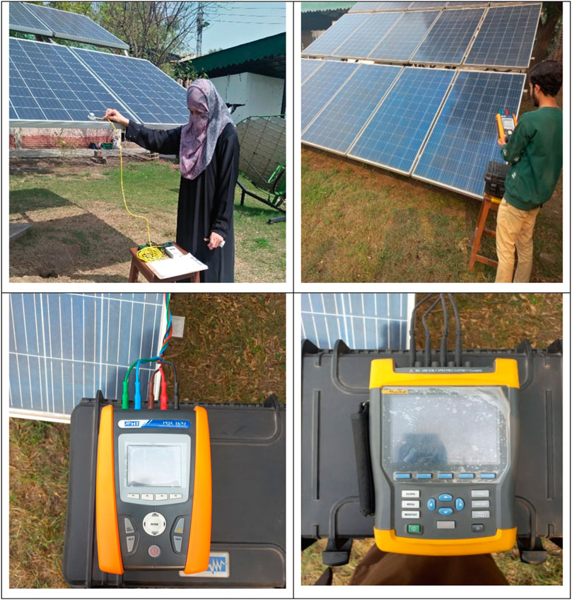
FIGURE A1. Experimental performance and instrumentations for fixed and tracked systems.
Keywords: photovoltaic, solar tracking system, three-point manual tracking, performance ratio, standard temperature and conditions
Citation: Saeed F, Ghafoor A, Hussain MI, Ikram K, Faheem M, Shahzad M, Amjad W, Omar MM and Lee GH (2024) Empirical and numerical-based predictive analysis of a single-axis PV system under semi-arid climate conditions of Pakistan. Front. Energy Res. 11:1293615. doi: 10.3389/fenrg.2023.1293615
Received: 13 September 2023; Accepted: 26 December 2023;
Published: 09 February 2024.
Edited by:
Peng-Yeng Yin, Ming Chuan University, TaiwanReviewed by:
Ammar Necaibia, Renewable Energy Development Center, AlgeriaHai Wang, Zhaoqing University, China
Copyright © 2024 Saeed, Ghafoor, Hussain, Ikram, Faheem, Shahzad, Amjad, Omar and Lee. This is an open-access article distributed under the terms of the Creative Commons Attribution License (CC BY). The use, distribution or reproduction in other forums is permitted, provided the original author(s) and the copyright owner(s) are credited and that the original publication in this journal is cited, in accordance with accepted academic practice. No use, distribution or reproduction is permitted which does not comply with these terms.
*Correspondence: Muhammad Mubashar Omar, bXViaV9tYWhtb29kQHlhaG9vLmNvbQ==; Gwi Hyun Lee, Z2hsZWVAa2FuZ3dvbi5hYy5rcg==