 Feifei Cui
 Dou An
 Yingzhuo Zhao
- School of Automation Science and Engineering, Faculty of Electronics and Information Engineering, Xi’an Jiaotong University, Xi’an, China
The home energy management system (HEMS), which utilizes multi-modal data from multiple sensors to generate the knowledge about decision making, is essential to the optimization of home energy management efficiency. Load scheduling based on HEMS can improve the utilization efficiency of multi-modal data and derived knowledge, achieve power supply-demand balance, and reduce users’ electricity costs. This paper proposes a distributed load optimization scheduling method for the load scheduling problem in HEMS based on multi-modal data-driven algorithm. Additionally, a two-stage data-driven optimization method is proposed, including a first-stage optimization model based on minimizing electricity costs and a second-stage optimization model based on minimizing system load fluctuations. In the first stage, cost self-optimization is performed based on energy storage devices. In the second stage, a load optimization instruction is issued by the control center, and each user optimizes the load fluctuations based on the system load data. Compared to centralized control methods, this approach reduces the computational overhead of the control center. Finally, simulation experiments based on load scheduling in the HEMS are conducted. The results of the first optimization stage show that when the battery capacity integrated into the system increases from 3.68 kWh to 6.68 kWh, user costs can be reduced from 57.572 cents to 42.064 cents. It is not only evident that the proposed method can effectively save users on electricity costs, but the introduction of larger capacity batteries also lowers these costs. The second stage of load fluctuation optimization results show that the proposed method can effectively optimize the usage data of a group of users and decrease the absolute peak-valley difference by 8.8%.
1 Introduction
1.1 Background
The next-generation smart grid is a network composed of digital systems and electrical infrastructure, capable of detecting multi-modal data from multiple sensors to monitor the status of energy usage. Additionally, the smart grid enables decision making technologies to reason the knowledge from multi-modal data to implement demand response and load dispatching functions, quickly and adaptively adjusting power generation and transmission (Mahela et al., 2022). The residential load is an essential part of the multi-modal data in smart grids, and as the application of residential load facilities increases, the energy consumption of residential loads continues to grow. Therefore, residential energy management is an urgent and crucial field that can enable end-users to actively participate in reshaping demand patterns.
A home energy management system (HEMS) is the product of the combination of smart grid intelligent communication and data-driven decision-making technology (Lin, 2021). HEMSs can effectively monitor household energy consumption through smart sensors and electronic devices and predict and plan home energy usage, thereby improving electricity utilization efficiency. To guide users to participate in demand response, power companies have introduced real-time pricing strategies in place of traditional fixed prices (Li et al., 2019). Real-time pricing plays an essential role in HEMSs, dividing the day into 24 or more time periods, achieving intelligent meter billing based on real-time prices (Wei et al., 2019). Governments and power grids collect detailed, real-time electricity data from customers via smart meters. This aids in balancing power generation with consumption, thereby stabilizing power system operations and reducing long-term production costs. Power companies set higher prices during peak hours and lower prices during off-peak periods, encouraging users to participate in power system operation management through real-time pricing. Users, aiming to reduce their energy costs, tend to use energy-saving appliances and shift their power usage from peak periods to non-peak periods, thereby improving energy efficiency while reducing electricity costs (Munankarmi et al., 2022). To promote two-way communication, advanced metering infrastructure (AMI) is an essential part of the smart grid’s HEMS (Lu et al., 2017), consisting of home area network (HAN), building area network (BAN), neighborhood area network (NAN), and other grid infrastructure (Huang et al., 2021).
Load scheduling based on HEMS can reduce energy consumption, save resources, save electricity costs for consumers and utilities, reduce greenhouse gas emissions, and reduce peak electricity demand. For example, Bejoy et al. (2017) proposed a household appliance scheduling method considering customer preferences and satisfaction to minimize energy consumption without causing inconvenience to users. Pal et al. (2017) used household electric vehicles to manage user load demand and proposed a framework including different appliance energy consumption loads, such as basic load, movable appliances, storage systems, and electric vehicle loads.
Although many achievements have been made in load scheduling based on HEMSs, the main method is to optimize the system load fluctuation by using the centralized control method, and the modeling of electrical equipment is not practical enough. This paper established the basic equipment and energy storage equipment models, and implemented user load scheduling through two-stage distributed data-driven optimization method. The main contributions are as follows:
• A distributed load scheduling framework for HEMS is proposed, and detailed modeling for various devices is conducted. In the distributed scheme, optimization control is decentralized to individual residential buildings or even to each household user, aiming to reduce the computational and communication overhead of the control center. HEMS is employed to facilitate bidirectional communication and distributed optimization.
• A data-driven two-stage optimization method is introduced. It aims to achieve demand response by optimizing for minimal user costs and minimal load fluctuations, respectively. In the first stage of distributed optimization, users’ demand response adjustments can create new peaks in the system load curve. users’ demand response adjustments can create new peaks in the system load curve. Users within an area share their optimized consumption from smart meters, and the control center releases system load directives. This prompts a secondary optimization where users exchange load data and iteratively adjust schedulable loads and battery statuses until load fluctuations remain within defined limits.
• Load scheduling simulation experiments were conducted, and the influence of battery parameters was analyzed. Simulation results indicate that, using the proposed method, users can adjust the load based on comfort levels and the urgency of device usage. The obtained scheduling strategy can effectively reduce user costs and decrease load fluctuations.
1.2 Research status
Residential users are a highly important component of the smart grid, accounting for 33% of total electricity consumption. Load scheduling based on home energy management systems (HEMSs) implements demand response from the resident side, and the implementation process faces many challenges, such as privacy leakage, randomness and management complexity of generation and consumption equipment. Therefore, researchers have introduced solutions based on energy storage devices (Seal et al., 2023), distributed energy (Chen and Chang, 2023), flexible loads (Yang et al., 2020), etc. Load scheduling based on HEMS can reduce energy consumption, save resources, save electricity costs for consumers and utilities, reduce greenhouse gas emissions, and reduce peak electricity demand.
Bejoy et al. (2017) proposed a household appliance scheduling method that considers customer preferences and satisfaction to minimize energy consumption without causing inconvenience to users. Pal et al. (2017) used household electric vehicles to manage user load demand and proposed a framework that includes different appliance energy consumption loads, such as basic load, movable appliances, storage systems, and electric vehicle loads. In the optimization process, each user can arrange their devices based on actual electricity usage. The scheme adds a bias cost to the objective function in the user cost minimization problem to prevent the formation of new peaks during non-peak periods, but using centralized control methods increases the computational burden of the system. Jiang and Wu (2020) proposed a cost-efficient load scheduling method considering user electricity efficiency and satisfaction, balancing user cost and preferences through fractional programming. Kou et al. (2019) introduced a distributed control scheme based on aggregators to achieve residential demand response. In this scheme, the power company provides an incentive price to drive power consumption adjustment based on the aggregated load information exchanged between the utility system and users. Wang et al. (2020) proposed a stochastic optimization method to solve the residential load scheduling problem, establishing residential load models, generation cost prediction models, and stochastic optimal load aggregation models. They introduced a set of uniformly distributed scalars to the load aggregation model to avoid load bounce, and experiments proved that this method effectively reduced the system’s load peak-average value. Yang et al. (2018) introduced a privacy-aware scheduling model based on rechargeable batteries, introducing coefficients to enable users to balance privacy protection and cost. The model uses the storage and release of energy by rechargeable batteries to flatten the user’s electricity curve and discusses the impact of battery capacity on privacy protection effects. Sangswang and Konghirun (2020) integrated solar energy, energy storage, and V2G. This study provided an optimized control method for electric vehicles and household batteries, enhancing the effectiveness of HEMS. Joo and Choi (2017) proposed a two-stage optimization algorithm for energy consumption scheduling in multiple smart homes under distributed energy. However, this study only considered the interests of consumers and overlooked the quality of the electrical grid. Awad et al. (2015) proposed load scheduling privacy protection methods based on rechargeable batteries and the maximum difference method, using the demand response component to keep the electricity curve constant, and proved that fuzzy processing of smart meter values does not affect user billing. Ming et al. (2016) introduced a user-side load scheduling method that considers user satisfaction, achieving demand response and user cost reduction through two-stage optimization, but did not consider the impact of distributed energy on the smart grid’s demand response. The model presented in this paper is a nonlinear programming problem, with variables encompassing both binary and continuous types, and it possesses complex constraints. While some traditional optimization algorithms, such as simulated annealing (Li et al., 2022) and particle swarm optimization (Zhao and Li, 2020), exhibit strong global search capabilities when dealing with nonlinear optimization problems, they encounter challenges when addressing mixed variables, multiple constraints, or high-dimensional problems. Genetic algorithms, on the other hand, can handle both discrete and continuous variables, making them suitable for a wide range of intricate optimization challenges. Therefore, this paper employs the genetic algorithm for model optimization.
2 Home energy management system
2.1 Framework of HEMS
The HEMS (Duman et al., 2021), an essential component of the smart grid, is a microgrid system composed of renewable energy generation equipment, energy storage devices, and various common household appliances. HEMS enables residential end-users to actively participate in reducing peak demand and carrying out demand response. Energy use can be shifted to non-peak periods by scheduling household appliances, reducing excessive energy consumption at certain times. Meanwhile, device scheduling operations must consider customer preferences and satisfaction to achieve the best results in energy scheduling optimization, for example, using air conditioning to maintain the indoor temperature within an appropriate range. To ensure the secure transmission of electricity data and costs between users and the smart grid within the HEMS, advanced metering infrastructure (AMI) is the foundation of HEMS. AMI consists of the home area network (HAN), building area network (BAN), neighborhood area network (NAN), and other grid infrastructure such as smart meters (Huang et al., 2021). The framework of the HEMS is shown in Figure 1.

FIGURE 1. Framework of HEMS.
The framework includes smart meters (SMs), gateways (GWs), control center (CC) of the power company, and users connected to the meters. Smart meters (Fekri et al., 2021) act as a home local area network, installed at the user’s end. They are connected to sensor devices in the home and collect user power consumption data through smart appliances, uploading it to the local gateway. Users can monitor and optimize energy control of electrical devices through the home main controller, understand energy usage and related data through smart meters, and choose appropriate electricity usage based on this information to enjoy high quality service. The gateway is a powerful entity used not only for relaying but also for data processing. The control center processes user electricity consumption, encrypted electricity costs, and other data sent from the gateway, and updates real-time prices based on total user electricity consumption, carrying out demand response to keep the load within a certain range in the area, thereby ensuring safe and reliable electricity use. During the transmission process of electricity consumption, for electricity cost-related privacy data, both the gateway and control center will carry out signature authentication to ensure data security and integrity. Users can view their billing accounts through the client and may choose to apply for verification.
2.2 Types of HEMS devices
The devices of HEMSs can be classified as basic devices or energy storage devices.
Basic devices are primarily focused on heating, ventilation, and air conditioning (HVAC), as well as washing machines, refrigerators, rice cookers, etc. Basic devices are divided into schedulable and non-schedulable devices. Non-schedulable devices, such as laptops and desk lamps, must meet users’ immediate usage needs, so their operation time cannot be controlled; therefore, non-schedulable devices are not modeled.
Energy storage devices can stitch together intermittent renewable energy and enhance the security and stability of the power supply system. They can also charge energy storage devices using the grid during off-peak electricity times, store electrical energy through certain mediums, and release the stored energy for power generation during peak electricity periods for household appliance use. This promotes peak shaving and valley filling in the grid, improving the reliability of the user’s power supply. Energy storage technologies typically include physical energy storage (flywheel energy storage, pumped hydro storage), chemical energy storage (various types of batteries, renewable fuel cells, supercapacitors), and electrical energy storage (superconducting electromagnetic energy storage). As a load balancing device and backup power source, energy storage systems are also essential equipment for smart grids and distributed energy systems.
3 Distributed system devices model
In the distributed scheme, optimization control is dispersed to individual residential buildings or even individual household users, as shown in Figure 2. Assume that there are W household users in the region, and in a household, in addition to basic electrical devices, energy storage devices are equipped. The home management system is used to provide two-way communication and distributed optimization. In the distributed load scheduling model, the control center is responsible for the publication of real-time electricity prices, system load instructions, and system load data; users can adjust their electricity usage patterns according to different electrical devices in the home, conduct electricity cost self-optimization, and then transmit the smart meter power consumption values to the control center. Furthermore, users transmit system load data to each other to perform system load fluctuation optimization sequentially. Compared to the centralized control scheme, the distributed control scheme reduces the computational and communication overhead of the control center and provides a scalable architecture.
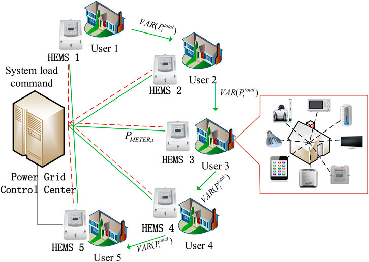
FIGURE 2. Distributed optimization-based load scheduling framework.
3.1 Schedulable devices model
Basic devices in the home, such as computers, incandescent lights, televisions, and other appliances that users need to use at any time, are considered non-schedulable devices. Adjusting their usage time would seriously affect users’ comfort, so they are not involved in load control. Schedulable devices, such as refrigerators and dishwashers, are referred to as having flexible loads. They can participate in demand response, and their flexibility can alleviate the strain on the power grid during peak electricity usage periods.
In this paper, a day is divided into H intervals, where h = 1, 2, ⋯H. The length of each interval is
To make the model closer to the actual situation, consideration is given to subdividing the devices.
3.1.1 Non-interruptible devices
Among the schedulable appliances, devices such as washing machines and rice cookers are considered non-interruptible devices. During operation, they are continuously powered by distributed energy or the grid, and once started, they cannot be stopped, as this would affect the normal functioning of the device. Therefore, once turned on within the schedulable range, they must continue for the specified working duration to complete the corresponding tasks. In addition to satisfying Eq. 1 and Eq. 2, they must meet the following time constraints:
3.1.2 Interruptible devices
Interruptible appliances require intermittent power supply from distributed energy or the grid. Each power supply duration should not be less than the minimum supply time (typically the minimum interval is 30 min or 15 min). With the condition of meeting the minimum interval, these devices can be turned on or off at any time. Examples include microwaves and air conditioners. In addition to satisfying Eq. 1 and Eq. 2, they must meet the following time constraints:
3.1.3 Constant power devices
Due to the significant proportion of HAVC equipment, such as air conditioners, in household electricity consumption, its power varies continuously over time. In contrast, appliances such as refrigerators generally operate at their rated power. Therefore, they are modeled separately. Assume that when a device starts, the power is Pa, and when idle, the power is 0. The power of a constant power device is given by:
3.1.4 Power-adjustable devices
Power-adjustable devices, such as temperature-controlled appliances like air conditioners, have power needs that vary continuously and are related to the outdoor temperature. The input parameter for the air conditioner is the day-ahead outdoor temperature, and its mathematical model is represented as:
where Tin(h) is the indoor temperature of time slot h; ɛ is the inertia coefficient of the indoor temperature change; Tout(h) is the outdoor temperature of time slot h; A is the thermal capacity of the room; PNC(h) is the rated power of the air-conditioning appliance in time slot h; η is the thermal conductivity efficiency of the room.
When the air conditioner operates in cooling mode, the value of ± in the formula is set to −; when the air conditioner operates in heating mode, the value of ± in the formula is set to +. Considering user comfort, the indoor temperature should be maintained within the range of user demand, and air-conditioning appliances must to satisfy the following constraints:
where
where
3.2 Energy storage devices model
Energy storage devices can store electrical energy through a certain medium, acting as a buffer between power generation and consumption. This enables users to charge and store energy during off-peak periods and utilize battery-released energy during peak periods, enhancing electricity safety and stability. The primary energy storage device used in homes is the lithium battery.
The main parameters affecting battery operation include: Capacity, State of Charge (SOC) and Charging or Discharging Power of the Battery.
3.2.1 Capacity
Capacity refers to the quantity of electrical charge a battery can store. It is denoted by Ebatt and is measured in ampere-hours, abbreviated as Ah. Generally, the larger the battery volume, the higher its capacity.
The rated capacity refers to the minimum amount of electrical energy released by the battery at 25°C when discharged at a 10-h rate.
The actual capacity represents the energy a battery can output under certain conditions, equivalent to the product of the current and time.
3.2.2 SOC
The state of charge reflects the ratio of the remaining battery charge to the battery’s capacity. To extend a battery’s lifespan, its state of charge must be considered during operation to ensure it remains within a certain range. When SOC = 0, the battery is depleted, and when SOC = 1, the battery is fully charged.
where SOC(h) represents the state of charge of the battery in time slot h; EB(h) is the remaining charge of the battery in time slot h; Ebatt is the battery capacity.
The charge of the battery in time slot h is calculated according to Eq. (10):
where EB0 is the initial charge of the battery; PB(h) is the charge/discharge power of the battery in time slot h.
The state of charge of the battery is influenced by its charging and discharging, and the dynamic change process is described in Eq. (11):
where
An excessively high or low SOC is detrimental to the battery’s lifespan. Therefore, constraints on the SOC range are shown in Eq. (12):
where SOCmin is the minimum allowable state of charge for the battery, SOCmax is the maximum allowable state of charge for the battery. When the battery’s state of charge falls below SOCmin, the battery will no longer discharge; when the state of charge exceeds SOCmax, the battery will no longer charge.
3.2.3 Charging or discharging power of the battery
When the battery is in operation, it is either in a charging state or in a discharging state. A 0–1 variable a is introduced to represent the state of the battery. b indicates the battery is in a charging state during time slot h, while c indicates the battery is in a discharging state during time slot h. To extend the battery’s lifespan, one cannot arbitrarily switch between charging and discharging states. Therefore, this paper maintains that a state switch can occur only after controlling the charging or discharging state for more than 30 min.
The constraints for the charging and discharging power of the battery in each time slot are shown in Eq. 13 and Eq. 14:
where ηch is the charging efficiency of the battery;
The charging and discharging power of the battery is:
In the equation, when the battery is in a charging state,
4 Two-stage distributed optimization model
4.1 First-stage optimization model
Each user household engages in flexible load scheduling, autonomously choosing their electricity consumption time. They opt to use electricity during low tariff periods, ensuring their electricity needs are met and thereby reducing household electricity costs. In the model of this paper, the smart grid can exchange electricity bidirectionally with users. That is, users can sell their excess energy back to the main grid. The optimization objective for minimizing electricity costs is expressed as:
where RTP(h) is the real-time electricity price published by the power grid company; PMETER(h) is the power consumption value recorded by the smart meter during time slot h.
In a Grid-Feeding HEMS, PMETER(h) can take both positive and negative values. When PMETER(h) is positive, the household is purchasing electricity from the grid. Conversely, when PMETER(h) is negative, the household is feeding electricity back to the grid. Users can obtain real-time electricity prices RTP(h) in advance from the power grid company.
The calculation method of PMETER(h) is shown in Eq. (17):
where PLOAD(h) represents the total load of basic household electrical appliances; PB(h) represents the battery’s charging and discharging quantity; PM(h) is the power consumption of non-dispatchable loads; PC(h) is the power consumption of power-stable devices among dispatchable loads; and PNC(h) is the power consumption of power-adjustable devices among dispatchable loads.
4.2 Second-stage optimization model
Each household user, in order to save costs, participates in demand response and adjusts their own electricity consumption behavior, which might introduce new peak demand for the system. To ensure the safe and stable operation of the grid and prevent this situation, the model takes into account the collective residential load in a specific region and incorporates system deviation costs into the objective function to minimize. This approach reduces the peak-to-average-power ratio (PAR) and prevents the system from encountering new peaks during non-peak periods.
The optimization objective for minimizing load fluctuation is expressed as:
where Costelec represents the user’s self-optimized electricity cost; γ is the weight factor of the deviation cost; w refers to a user in household w. The second term of the function, denoted as
Final model output:
1) The (A + 3) × H-dimensional flexible load state matrix XChrom represents the working status of all flexible loads over a 24-h day after participating in load scheduling, as shown in Eq. (21):
where XChrom is a matrix composed of XSa, XSB, XPT and XPB. Matrix XSa (a = 1, 2, ⋯A) represents the working status of device a, with 0 indicating working and 1 indicating idle. Vector XSB represents the working status of the battery. Vector XPT represents the power of adjustable power devices. Vector XPB represents the charge and discharge power values of the battery.
2) All flexible load working states multiplied by the rated power of the corresponding time slot result in the power consumption of the adjustable device for each time slot in a day. This is referred to as the power consumption matrix PChrom, as shown in Eq. (22):
After HEMS load scheduling, the obtained adjustable device state matrix XChrom and power consumption matrix PChrom represent the optimal working state collection that satisfies both the device’s inherent constraints and user comfort.
5 Load scheduling based on two-stage distributed optimization
5.1 Scheduling process based on two-stage distributed optimization
One commonly used method to reduce user costs and mitigate system load fluctuations through load scheduling is centralized control. Power company control centers process the power consumption values collected from smart meters in a given region, thereby decreasing system peak averages and smoothing the system load curve. However, centralized control methods present certain challenges. The computational burden at the control center, coupled with the communication overhead from each user transmitting to the center, is considerable. This is primarily because the load state matrix XChrom of (A + 3) × H dimension for each user in the region forms a three-dimensional matrix (A + 3) × H × W, where W is the number of users. All require optimization computations through the control center. As the number of users grows, the computational scale of the aforementioned model substantially increases. Employing distributed optimization control methods can circumvent the curse of dimensionality. Additionally, distributed optimization methods offer robust user privacy protection. Users only need to upload the post-optimization smart meter values, with each household independently optimizing load fluctuations. The data transmitted between users pertains to system load, negating the need for individual household power data. In contrast, centralized control mandates not just the uploading of smart meter consumption data, but also the power and status of each appliance in a household. By readjusting the power and status of appliances, the control center minimizes system load fluctuations. In doing so, it gains access to granular user consumption data, which inevitably breaches user privacy.
Distributed optimization facilitates a layered, phased approach to the optimization process. In this paper’s distributed optimization load scheduling model, the first phase encompasses users self-optimizing for cost. Under the premise of ensuring user comfort, the electricity usage time of flexible loads is adjusted to minimize each household’s electricity cost. Subsequently, the optimized smart meter consumption values are uploaded. Some of the literature has explored the gradual processing of smart meter consumption values to better safeguard user privacy. The second phase focuses on optimizing system load fluctuations. The control center processes the collected regional smart meter consumption values to obtain aggregate area electricity consumption and system load fluctuation data. The power company’s control center then releases system load optimization command
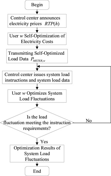
FIGURE 3. Distributed optimization-based load scheduling process.
5.2 Model resolution based on hybrid coding genetic algorithm
Eq. (18) is a nonlinear programming problem. Typical optimization model solutions can use methods such as simulated annealing or particle swarm optimization. However, due to the uniqueness of variables in this paper’s model, as indicated by Eq. 21 and Eq. 22, the variables to be resolved include both binary 0–1 variables and continuous variables. Moreover, it possesses stringent constraint conditions. When using a genetic algorithm, the total number of 1’s in a chromosome represents the equipment’s operating duration. By controlling the positions of 1’s in the chromosome, we can set the equipment start and stop times, thus determining its scheduling range, which is in line with the schedulable model. The genetic algorithm demonstrates superior performance in handling this paper’s model, hence its selection.
The use of genetic algorithms to solve optimization problems comprises four main steps: potential solution encoding, initial population gene initialization, fitness function computation, and genetic operations. These operations include selection, replication, crossover, and mutation. In this paper’s model, apart from the conventional upper and lower limit constraints, there are some unconventional constraints. All electric devices must adhere to the constraints of Eq. 1 and Eq. 2. Non-interruptible devices must comply with the constraints of Eq. (4), which restricts the number and position of occurrences of 0 and 1 values in genes. Traditional genetic algorithms cannot resolve this problem. Modifications are required for potential solution encoding, population generation, and crossover mutation, necessitating the use of a hybrid coding genetic algorithm.
5.2.1 Initial population
5.2.1.1 Hybrid encoding
In the HEMS model of this paper, the operating status of schedulable devices is a discrete variable, represented by 1 when in operation and 0 when idle. The battery’s working state is also a discrete variable, represented by 1 during charging and 0 during discharging. However, the power of adjustable power devices such as air conditioners and the charging and discharging power of batteries are continuous variables, denoted as XPT and XPB, respectively. Therefore, the chromosome composition of an individual is shown in Eq. (23):
where XChrom is a chromosome group composed of XSa, XSB, XPT and XPB. H represents the day divided into H time slots. The binary encoded chromosome XSa (a = 1, 2, ⋯A) denotes the working status of device a. The binary encoded chromosome XSB indicates the working status of the battery. The real-number encoded chromosome XPT is the power of adjustable power devices. The real-number encoded chromosome XPB stands for the charging and discharging power of the battery.
Suppose the initial population size is K and that the length of each chromosome is H. The initial population can then be depicted using a three-dimensional matrix X with a size of (A + 3) × H × K.
XSa must satisfy the constraints of Eq. 1 and Eq. 2, where the number 1 can only appear between the αa-th and βa-th positions in XSa, and the total count of 1s is equal to da. For non-interruptible appliances, Eq. (3) must be satisfied, where gene 1 can only appear continuously between the αa-th and βa-th positions. The interruptible appliances satisfy Eq. (4), with gene 1 appearing randomly between the αa-th and βa-th positions. The operating power of the air conditioner XPT and the charge-discharge power of the battery XPB must also adhere to their respective upper and lower power limits.
5.2.1.2 Fitness function
The fitness function is used to evaluate an individual’s adaptability to its environment, determining the probability of its genes being passed on. This directly affects whether the optimal solution can be found and the convergence speed of the algorithm. The design should be as simple as possible to minimize computational complexity. To apply the genetic algorithm for solution finding, the problem of maximizing the objective function should be transformed into a minimization problem. In the model presented in this paper, the objective functions F for the two phases of distributed optimization take non-negative values. The fitness function is chosen as the reciprocal of the objective function. In the first phase, where users optimize themselves, the fitness function is taken as the reciprocal of the cost function. In the second phase of load fluctuation optimization, the fitness function is the reciprocal of the variance of system load data. Therefore, the fitness function f can be represented as:
5.2.2 Genetic operations
5.2.2.1 Selection
After calculating the fitness of all individuals, the selection process determines which individuals will participate in reproduction and pass their genes on to the next-generation. Individuals with a high fitness value have a greater chance of being selected, while those with a low fitness value have a lesser chance. Roulette wheel selection is commonly used for this purpose. The probability Pxi of individual xi being selected is calculated according to Eq. (25):
where fi is the fitness of the first individual; K stands for the total number of individuals in the population.
5.2.2.2 Crossover
Crossover, or genetic recombination, involves taking two parent individuals and swapping portions of their chromosomes to produce two new chromosomes, thereby creating new offspring individuals. The crossover probability Pc is typically a random number between 0 and 1. Consequently, the probability of the parent chromosomes being directly copied to the next-generation is 1 − Pc.
In the model presented in this paper, there are both binary-encoded chromosomes and real-number encoded chromosomes. Accordingly, the crossover method should be chosen to match the respective encoding types.
For binary-encoded chromosomes of basic devices, one or multiple crossover points are selected on the parent chromosomes, followed by a swapping operation. It is crucial to ensure that after crossover, the constraints for non-interruptible devices given by Eq. 3 and for interruptible devices given by Eq. (4) are still satisfied.
For chromosomes corresponding to power-adjustable devices and rechargeable battery power encoded in real numbers, calculations are performed with a random number between 0 and 1 and the parental chromosome. If the parental chromosome is represented by
5.2.2.3 Mutation
Mutation refers to the periodic random updating of a gene on a chromosome to refresh the population, exploring unknown areas in the solution space.
In the model of this paper, for binary encoded chromosomes, when a random number is less than the mutation probability Pm, the corresponding chromosome’s binary string is flipped. When the original gene value at the mutation point is 0, it is flipped to 1; when the original gene value at the mutation point is 1, it is flipped to 0. For real-number encoded chromosomes, a uniformly distributed random number within the value range replaces it, namely, the uniform distribution method. The calculation method for the mutated gene is based on Eq. (27):
where
The algorithm flow of the genetic algorithm is shown in Figure 4.
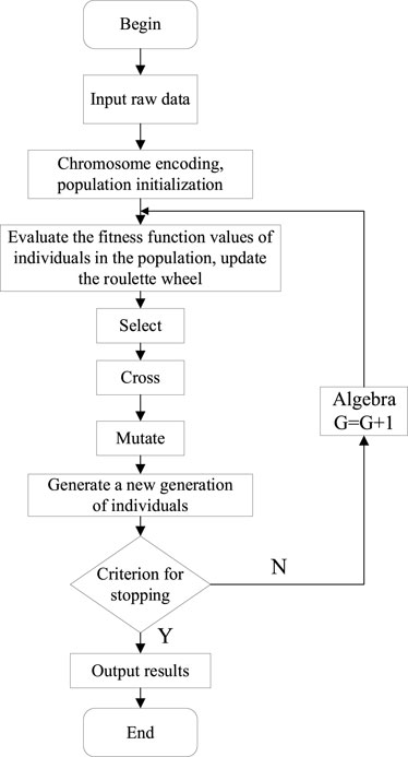
FIGURE 4. Genetic algorithm Flowchart.
6 Simulation verification
To conduct research on load optimization scheduling for the HEMS, this study designed a distributed optimization load scheduling simulation experiment. In the first phase, users optimize costs for themselves, while in the second phase, the optimization focuses on reducing the system’s load fluctuations. The study also investigates the impact of energy storage devices on load scheduling.
6.1 Parameter settings
Dividing the 24-h day into 48 time intervals results in Δhstep = 30 min. Python was used for modeling and solving. The simulation platform was equipped with an Intel(R) Core(TM) i5-10400 CPU at 2.90 GHz, 16 GB of RAM, and ran Windows 10 Home edition as its operating system. The output variables of the experiment are the flexible load status matrix, from which the power consumption matrix of various electrical devices, the consumption values of the smart meter, and the daily electricity costs can be deduced. The data sources and settings are described as follows.
6.1.1 Electricity prices and outdoor temperature data
The outdoor temperature data are taken from the temperature readings of a particular summer day in Xi’an. The electricity prices and outdoor temperature data are shown in Figure 5A, B, respectively.
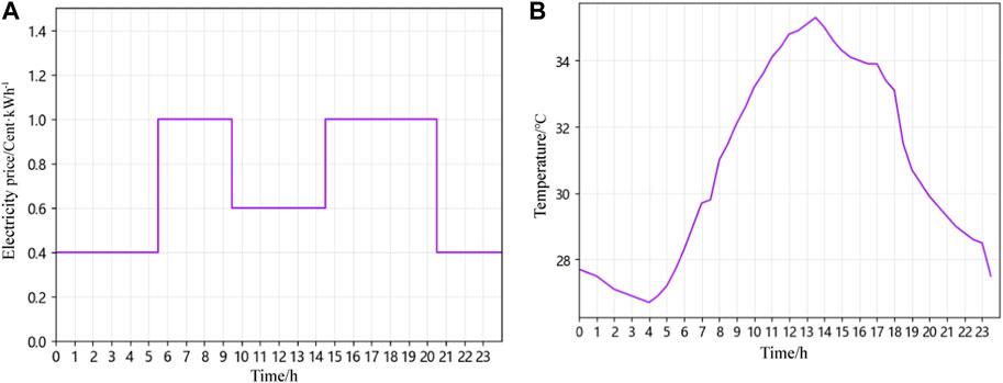
FIGURE 5. Electricity prices and outdoor temperature data: (A) real-time electricity price; (B) outdoor temperature variation curve.
6.1.2 Parameter settings for dispatchable devices
The primary device chosen for power-adjustable research is the air conditioner. The temperature parameters ɛ, A and η for the air conditioner are set to 0.93, 2.5, and 0.45, respectively. In the summer, the air conditioner operates in cooling mode, and its maximum allowed power output per time slot is 3.6 kWh. The indoor temperature set by the user must be maintained between 24°C and 26°C.
Power-fixed devices include 20 basic devices, of which device number 2, the washing machine, and device number 16, the rice cooker, are non-interruptible devices. These devices must adhere to the respective time constraints of non-interruptible devices; once activated, they must complete their respective tasks before they can stop. The remaining 18 devices are interruptible. All device tasks are numbered, and the dispatch time range, working duration, and power of dispatchable devices are presented, as shown in Table 1:
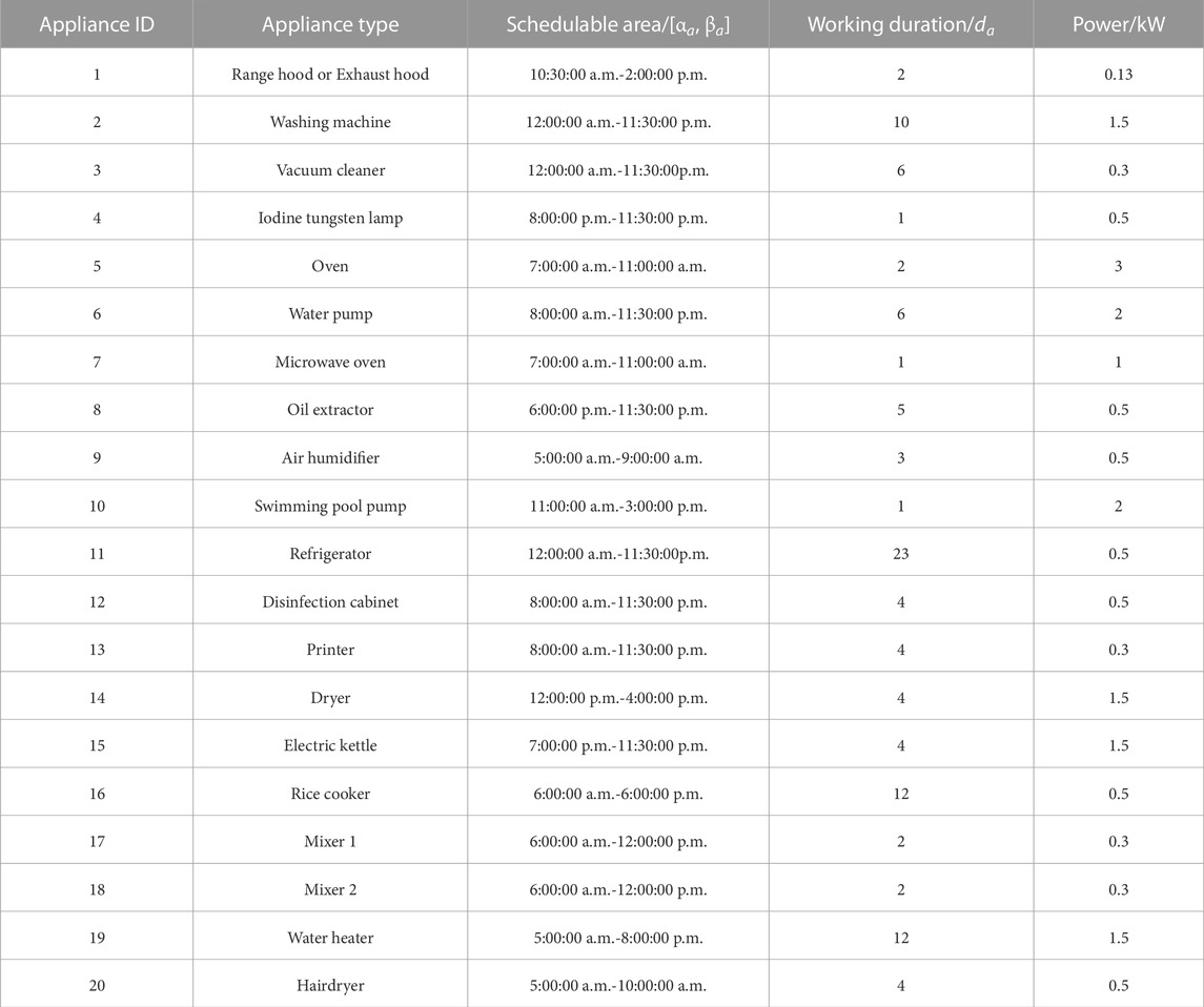
TABLE 1. Parameter settings for dispatchable devices.
6.1.3 Energy storage device parameter settings
The energy storage device selected is a household lithium battery. There are two types of batteries: Battery A has a capacity of 3.68 kWh and a maximum charging/discharging power of 2.5 kW; Battery B has a capacity of 6.68 kWh and a maximum charging/discharging power of 5 kW. The SOC of the battery must be maintained between 0.3 and 0.9.
6.1.4 Genetic algorithm parameter settings
In the initialization parameters of the genetic algorithm, the population size N = 50. Thus, the initial population can be represented by a three-dimensional matrix X (size: 23 × 48 × 50). The crossover probability Pc = 0.8, mutation probability Pm = 0.1, and the maximum number of iterations is 150 times.
6.2 First-stage simulation results
The original electricity load curve of a household user within 48 time slots in a day is shown in Figure 6A. At this time, the electricity cost is 115.566 cents. As can be seen from the figure, the user’s electricity consumption is concentrated in 6:00–10:30. A significant portion of this time falls within the higher electricity price period, such as 6:00–9:30. Therefore, the user’s electricity cost is relatively high.
Figure 6B displays the electricity scheduling results for various adjustable devices over the 48 time slots of a day through a heatmap. Taking the vacuum cleaner as an example, its usage time reaches 2.5 h during the high electricity price periods of 5:30–9:30 and 14:30–20:30.
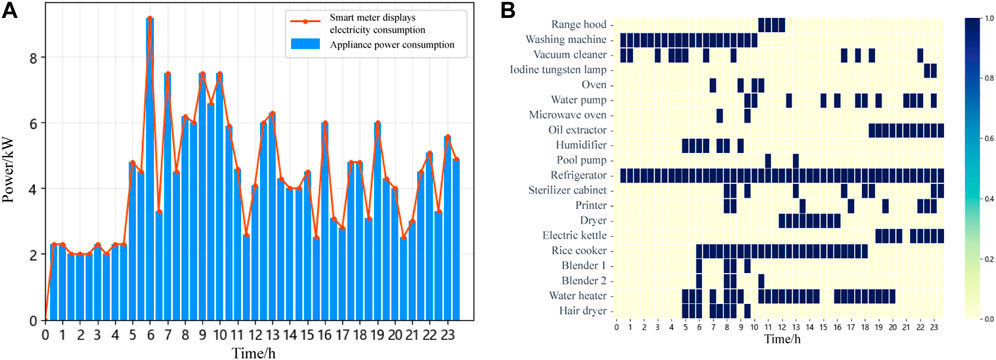
FIGURE 6. Electricity prices and outdoor temperature data: (A)initial electricity load curve; (B)operational status diagram of electrical devices.
1) Scenario I: No battery storage is integrated into the system.
The electricity task scheduling simulation results without battery storage integration are shown in Figure 7B. The household electricity cost is 72.716 cents. Since there is no energy storage device connected, the amount of electricity exchanged with the grid for each time slot equals the consumption value from the smart meter. The figure shows that the peak electricity consumption periods are concentrated around 7:30–10:00, 12:00–12:30, and 13:30–15:00. The real-time electricity price plays a dominant role, and to save costs, users shift their electricity consumption to periods with lower prices, such as 9:30–10:00, 12:00–12:30, and 13:30–14:30. Figure 7A illustrates the indoor temperature variation curve. As shown, the indoor temperature remains within the user-defined range of 24°C–26°C.
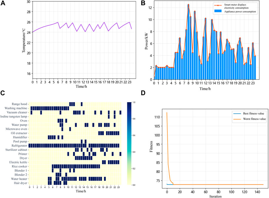
FIGURE 7. Simulation results without energy storage battery integration: (A) indoor temperature variation curve; (B) electricity task scheduling results; (C) operational status diagram of electrical devices; (D) convergence curve of genetic algorithm.
Figure 7C displays the electricity scheduling results of various dispatchable devices over the 48 time slots in a day using a heatmap. As illustrated by the chart, the washing machine and rice cooker, being non-interruptible devices, must complete their respective tasks once they start before they can stop. The working hours of the dispatchable devices have been adjusted accordingly. For instance, the vacuum cleaner’s usage during the high electricity price periods has been reduced to 1.5 h.
Figure 7D displays the convergence curve of the genetic algorithm; the improved genetic algorithm converges relatively quickly.
2) Scenario Π: System connected to Battery A or B
(1) Connection to Battery A
With the system integrated with Battery A, the electricity cost is 57.572 cents. The load scheduling simulation result is shown in Figure 8A. With the integration of a battery, the user can sell surplus electricity back to the grid. Thus, the system’s feed-in capability can enhance the overall economic benefits of the system. At this point, the smart meter’s displayed electricity consumption includes the electricity consumption of basic appliances and the rechargeable battery. The chart shows that the user sells electricity to the grid between 3:00 and 3:30. The electricity scheduling result now depends not only on real-time electricity prices but also on the battery’s charging and discharging behavior. When the battery is charging, the power is positive, and when discharging, the power is negative. Figure 8B reveals that through energy storage with the battery, it charges during low-price phases such as 0:00–0:30, 1:30–2:30, 3:00–5:00, 9:30–11:00, 14:00–14:30, 20:30–21:30, and 23:00–24:00. During high-price periods, it discharges energy for appliances, such as 5:30–6:30, 7:30–8:30, 14:30–16:00, and 18:00–19:30. The battery’s SOC value always remains between 0.3 and 0.9.
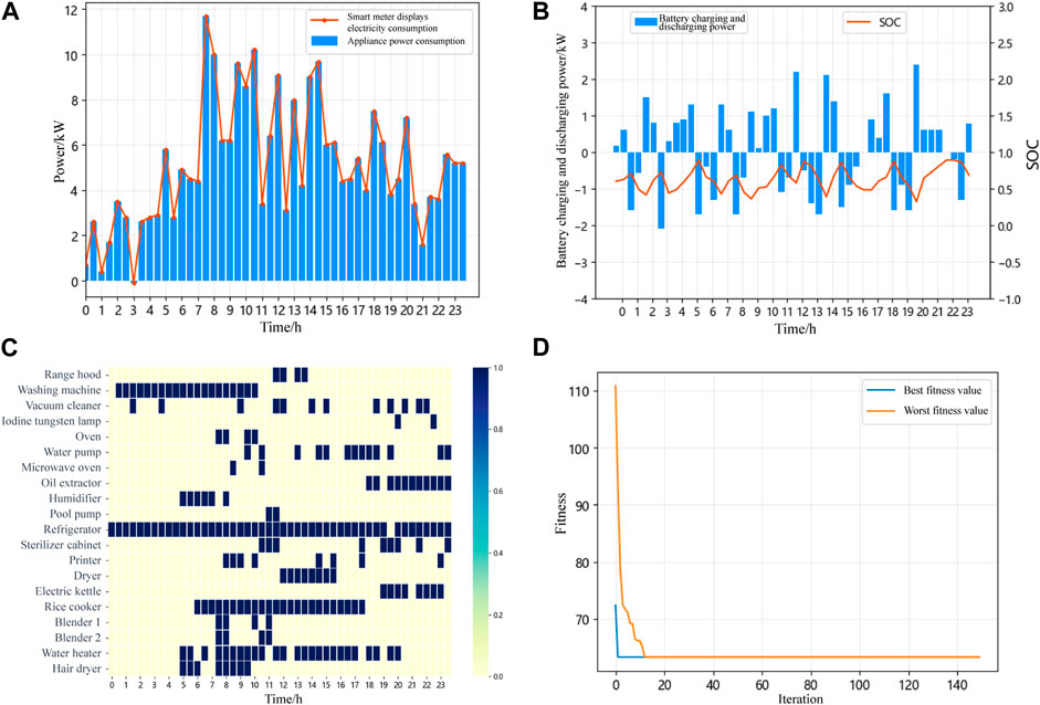
FIGURE 8. Simulation results with battery A integration: (A) electricity task scheduling results; (B) battery charging and discharging power and SOC; (C) operational status diagram of electrical devices; (D) convergence curve of genetic algorithm.
Figure 8C displays a heatmap showcasing the electricity scheduling results for various adjustable devices over a 24-h period with 48 time slots when the system is connected to a battery. There have been certain adjustments in the electricity usage of the appliances. Taking the vacuum cleaner as an example, its usage during the high electricity price intervals is reduced to 2 h. Figure 8D illustrates the convergence curve of the genetic algorithm.
(2) Connection to Battery B
The electricity cost now stands at 42.064 cents. This implies that the larger the capacity of the battery integrated into the system, the more it aids in leveling the peaks and troughs through energy storage, resulting in a lower electricity cost for the user. The energy scheduling simulation results are depicted in Figure 9A. The task allocation for electricity devices does not differ significantly from that when Battery A was incorporated, and there is not a significant difference in the frequency of battery charge-discharge cycles. Due to the larger capacity of Battery B, excess energy is sold back to the grid during the low-price intervals, such as 00:30–1:00, 2:30–3:00, 4:30–5:00, and 11:30–12:00, leading to even lower electricity costs. However, load scheduling based on battery storage resulted in a higher peak power demand. In the figure, the power demand peak is 7:00–7:30, and this peak value is even higher than the initial peak demand of the user, posing challenges for stable operation of the system. Therefore, subsequent optimization is required in the second phase to reduce system load fluctuations and prevent new electricity demand peaks.
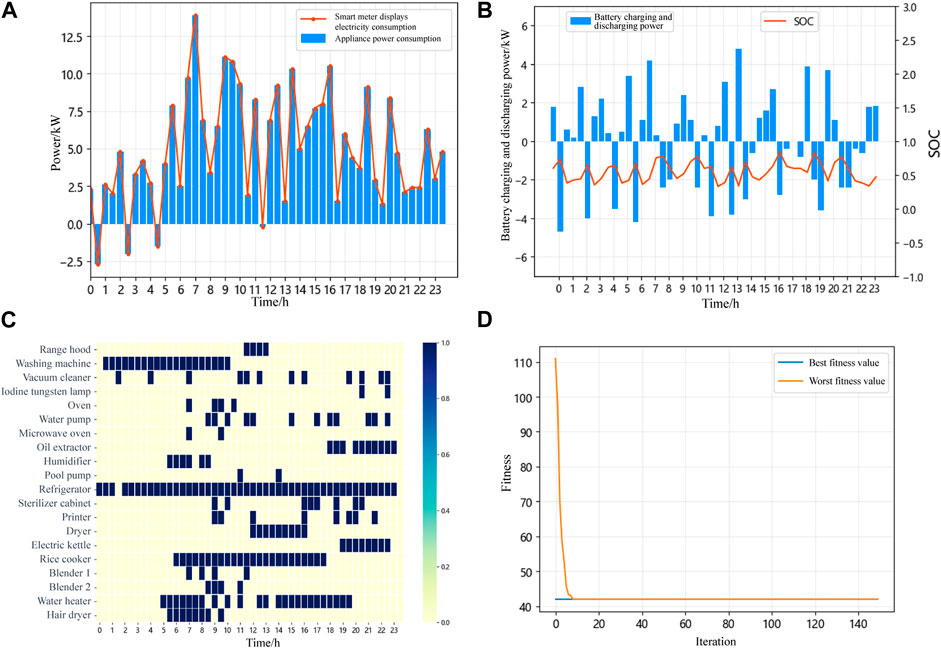
FIGURE 9. Simulation results with battery B integration: (A) electricity task scheduling results; (B) battery charging and discharging power and SOC; (C) operational status diagram of electrical devices; (D) convergence curve of genetic algorithm.
From Figure 9B, it can be observed that the battery is used for energy storage and is charged during the low-price intervals, such as 0:30–2:00, 2:30–4:00, 4:30–5:30, 9:30–10:00, 11:30–12:30, 13:00–13:30, 20:30–21:30, and 22:30–24:00, primarily in the early hours of the morning. During high-price intervals, such as 5:30–6:00, 7:30–8:30, 16:00–17:00, 17:30–18:00, and 18:30–19:30, the stored energy in the battery is released to power the devices. Similarly, the SOC of the battery consistently remains between 0.3 and 0.9.
Figure 9C displays a heatmap illustrating the electricity scheduling results of various schedulable devices over 24 h, divided into 48 time slots, when Battery B is integrated into the system. Adjustments can be observed in the usage times of devices such as the vacuum cleaner and the disinfection cabinet. Taking the vacuum cleaner as an example, its initial load usage during high electricity price periods was 2.5 h, which has now been reduced to 2 h. Figure 9D presents the convergence curve of the genetic algorithm.
6.3 Second-stage simulation results
Demand response can reduce user costs, but it might introduce new peak electricity demands to the system. Therefore, a second phase of distributed optimization is conducted to minimize system load fluctuations. Considering an area with W = 20 households, a distributed load fluctuation optimization simulation experiment is conducted. The energy scheduling mechanism’s impact on user electricity consumption behavior is analyzed from the perspective of a group of users. The energy storage system opted to integrate Battery A. The system load command is set at
Figure 10 shows the results of the system load fluctuation optimization simulation. As evident from the figure, after undergoing system load fluctuation optimization, compared to the self-optimization of user costs in the first phase, there is a significant change in the electricity consumption patterns of the user group within the area. The system load curve becomes more stable, with a reduction in peak values and an increase in valley values.
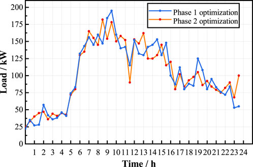
FIGURE 10. Optimization of system load curve at different stages.
Table 2 shows the electricity consumption behavior characteristics of the user group. The quality of system electricity consumption is assessed through indicators such as the load factor, which is the ratio of the average load to the peak load over a specific period. Improving the load factor can effectively reduce peaks, elevate valleys, decrease the peak-valley difference, and ensure the safe and stable operation of the power system. From Table 2, it can be observed that after the second-phase load fluctuation optimization, the system’s peak load decreased by 6.9%, the valley increased by 7.2%, the absolute peak-valley difference dropped by 8.8%, the peak-valley coefficient decreased by 13.2%, and the peak-valley difference rate reduced by 2.3%. Additionally, the load factor rose from 51.7% to 56.2%, an increase of 4.5%, and the variance of the load fluctuation decreased by 7.8%.
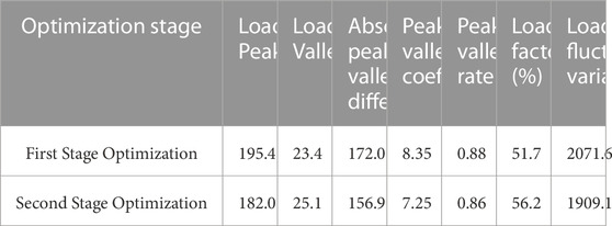
TABLE 2. System load parameter optimization at different stages for the user group.
Table 3 shows the user costs before and after distributed optimization. The average cost for users before and after distributed optimization decreased from 113.954 cents to 65.272 cents, a reduction of 42.7%. This shows that user costs decrease after distributed optimization. Compared to that in the first stage of optimization, the costs for some users increased because they made financial sacrifices to change system load fluctuations. Users can set the weighting factor γ as needed to balance cost and load fluctuation. Considering real-world scenarios, power companies can incentivize users who have increased costs, for instance, by reducing electricity prices, to encourage them to participate in optimizing load fluctuations.
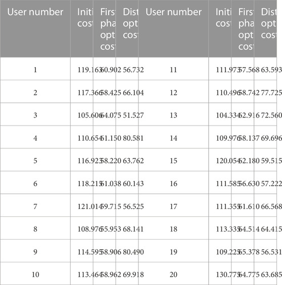
TABLE 3. Cost optimization for users at various stages.
7 Conclusion
This paper proposed a two-stage distributed optimization method for the HEMS based on data-driven algorithm. Firstly, a distributed load scheduling framework for HEMS is established, and various devices are modeled. Secondly, a two-stage optimization method is introduced, targeting both the minimization of user cost and load fluctuations to achieve demand response. Finally, simulation experiments of the load scheduling are conducted, and the impact of battery parameters on energy scheduling is analyzed. Simulation results demonstrate that users can adjust their loads based on comfort and the urgency of device usage. The main conclusions are as follows:
• The first optimization stage results indicate that when the battery capacity integrated into the system increases from 3.68 kWh to 6.68 kWh, user costs can be reduced from 57.572 cents to 42.064 cents. It is evident that not only can the proposed method effectively save electricity costs for users, but the introduction of larger capacity batteries also significantly reduces these costs.
• The second stage results indicate that, the system’s peak load decreases by 6.9%, the valley increases by 7.2%, and the absolute peak-valley difference is reduced by 8.8%. This demonstrates that the proposed method can effectively optimize the usage data of a group of users and decrease system load fluctuations.
Data availability statement
The original contributions presented in the study are included in the article/supplementary material, further inquiries can be directed to the corresponding author.
Author contributions
FC: Conceptualization, Investigation, Validation, Writing–original draft. DA: Funding acquisition, Project administration, Writing–review and editing. YZ: Investigation, Validation, Writing–review and editing.
Funding
The author(s) declare financial support was received for the research, authorship, and/or publication of this article. This work was supported in part by the National Natural Science Foundation of China under Grant 61803295; in part by the Major Research Plan of the National Natural Science Foundation of China under Grant 61833015.
Conflict of interest
The authors declare that the research was conducted in the absence of any commercial or financial relationships that could be construed as a potential conflict of interest.
Publisher’s note
All claims expressed in this article are solely those of the authors and do not necessarily represent those of their affiliated organizations, or those of the publisher, the editors and the reviewers. Any product that may be evaluated in this article, or claim that may be made by its manufacturer, is not guaranteed or endorsed by the publisher.
References
Awad, A., Bazan, P., and German, R. (2015). “Privacy aware demand response and smart metering,” in 2015 IEEE 81st Vehicular Technology Conference (VTC Spring) (IEEE), Glasgow, UK, 11-14 May 2015. 1–5.
Bejoy, E., Islam, S., and Oo, A. (2017). “Optimal scheduling of appliances through residential energy management,” in 2017 Australasian Universities Power Engineering Conference (AUPEC) (IEEE), Genre: Konferenzschrift, 19-22 Nov. 2017.
Chen, S.-Y., and Chang, C.-H. (2023). Optimal power flows control for home energy management with renewable energy and energy storage systems. IEEE Trans. Energy Convers. 38, 218–229. doi:10.1109/tec.2022.3198883
Duman, A. C., Erden, H. S., Gönül, Ö., and Güler, Ö. (2021). A home energy management system with an integrated smart thermostat for demand response in smart grids. Sustain. Cities Soc. 65, 102639. doi:10.1016/j.scs.2020.102639
Fekri, M. N., Patel, H., Grolinger, K., and Sharma, V. (2021). Deep learning for load forecasting with smart meter data: online adaptive recurrent neural network. Appl. Energy 282, 116177. doi:10.1016/j.apenergy.2020.116177
Huang, C., Wang, X., Gan, Q., Huang, D., Yao, M., and Lin, Y. (2021). A lightweight and fault-tolerable data aggregation scheme for privacy-friendly smart grids environment. Clust. Comput. 24, 3495–3514. doi:10.1007/s10586-021-03345-w
Jiang, X., and Wu, L. (2020). Residential power scheduling based on cost efficiency for demand response in smart grid. IEEE Access 8, 197324–197336. doi:10.1109/access.2020.3034767
Joo, I.-Y., and Choi, D.-H. (2017). Distributed optimization framework for energy management of multiple smart homes with distributed energy resources. IEEE Access 5, 15551–15560. doi:10.1109/access.2017.2734911
Kou, X., Li, F., Dong, J., Starke, M., Munk, J., Kuruganti, T., et al. (2019). “A distributed energy management approach for residential demand response,” in 2019 3rd International Conference on Smart Grid and Smart Cities (ICSGSC) (IEEE), Berkeley, CA, USA, June 25 2019 to June 28 2019, 170–175.
Li, C., Chen, Y., Yang, Y., Li, C., and Zeng, Y. (2019). “Ppcsb: a privacy-preserving electricity consumption statistics and billing scheme in smart grid,” in Artificial Intelligence and Security: 5th International Conference, ICAIS 2019, New York, NY, USA, July 26–28, 2019, 529–541.
Li, J., Guo, L., Zuo, Y., and Liu, W. (2022). A design method for wideband chaff element using simulated annealing algorithm. IEEE Antennas Wirel. Propag. Lett. 21, 1208–1212. doi:10.1109/lawp.2022.3161762
Lin, Y.-H. (2021). Trainingless multi-objective evolutionary computing-based nonintrusive load monitoring: Part of smart-home energy management for demand-side management. J. Build. Eng. 33, 101601. doi:10.1016/j.jobe.2020.101601
Lu, R., Heung, K., Lashkari, A. H., and Ghorbani, A. A. (2017). A lightweight privacy-preserving data aggregation scheme for fog computing-enhanced iot. IEEE access 5, 3302–3312. doi:10.1109/access.2017.2677520
Mahela, O. P., Khosravy, M., Gupta, N., Khan, B., Alhelou, H. H., Mahla, R., et al. (2022). Comprehensive overview of multi-agent systems for controlling smart grids. CSEE J. Power Energy Syst. 8, 115–131. doi:10.17775/CSEEJPES.2020.03390
Ming, Z., Geng, W., Haojing, W., Ran, L., Bo, Z., and Chenjun, S. (2016). Regulation strategies of demand response considering user satisfaction under smart power background. Power Syst. Technol. 40, 2917–2923. doi:10.13335/j.1000-3673.pst.2016.10.001
Munankarmi, P., Wu, H., Pratt, A., Lunacek, M., Balamurugan, S. P., and Spitsen, P. (2022). Home energy management system for price-responsive operation of consumer technologies under an export rate. IEEE Access 10, 50087–50099. doi:10.1109/access.2022.3172696
Pal, S., Kumar, M., and Kumar, R. (2017). “Price aware residential demand response with renewable sources and electric vehicle,” in 2017 IEEE International WIE Conference on Electrical and Computer Engineering (WIECON-ECE) (IEEE), Dehradun, India, 18-19 December 2017, 211. –214.
Sangswang, A., and Konghirun, M. (2020). Optimal strategies in home energy management system integrating solar power, energy storage, and vehicle-to-grid for grid support and energy efficiency. IEEE Trans. Industry Appl. 56, 5716–5728. doi:10.1109/tia.2020.2991652
Seal, S., Boulet, B., Dehkordi, V. R., Bouffard, F., and Joos, G. (2023). Centralized mpc for home energy management with ev as mobile energy storage unit. IEEE Trans. Sustain. Energy 14, 1425–1435. doi:10.1109/tste.2023.3235703
Wang, Z., Munawar, U., and Paranjape, R. (2020). “Stochastic optimization for residential demand response under time of use,” in 2020 IEEE International Conference on Power Electronics, Smart Grid and Renewable Energy (PESGRE2020) (IEEE), Le Méridien Cochin, Kerala, India, 2-4 Jan 2020.
Wei, H., Bo, Z., and Yubo, L. (2019). eal-time pricing scheme based on privacy protection. Appl. Res. Computers/Jisuanji Yingyong Yanjiu 36. doi:10.19734/j.issn.1001-3695.2017.12.0823
Yang, J., Huang, G., and Wei, C. (2018). Privacy-aware electricity scheduling for home energy management system. Peer-to-Peer Netw. Appl. 11, 309–317. doi:10.1007/s12083-016-0492-x
Yang, Z., Pu, Y., Liu, H., and Ni, M. (2020). “Optimal home energy management strategy considering integrated demand response,” in 2020 12th IEEE PES Asia-Pacific Power and Energy Engineering Conference (APPEEC), Nanjing, China, 20-23 September 2020.
Keywords: multi-modal data, home energy management system, knowledge reasoning, distributed optimization, real-time electricity pricing
Citation: Cui F, An D and Zhao Y (2023) A two-stage distributed optimization method for home energy management systems via multi-modal data-driven algorithm. Front. Energy Res. 11:1289641. doi: 10.3389/fenrg.2023.1289641
Received: 06 September 2023; Accepted: 23 October 2023;
Published: 03 November 2023.
Edited by:
Fuqi Ma, Xi’an University of Technology, ChinaCopyright © 2023 Cui, An and Zhao. This is an open-access article distributed under the terms of the Creative Commons Attribution License (CC BY). The use, distribution or reproduction in other forums is permitted, provided the original author(s) and the copyright owner(s) are credited and that the original publication in this journal is cited, in accordance with accepted academic practice. No use, distribution or reproduction is permitted which does not comply with these terms.
*Correspondence: Dou An, ZG91YW4yMDE3QHhqdHUuZWR1LmNu