Market power risk prevention mechanism of China’s electricity spot market based on stochastic evolutionary game dynamics

The construction of China’s power spot market is still in its early stage, with a high concentration on generation-side resources and frequent market power. It is urgent to establish risk prevention mechanisms for the generation of market power. First, the paper establishes a basic framework of the stochastic evolutionary game theory and then builds a “stochastic evolutionary game market-clearing” model for the market regulator and risk units. Second, the work provides a library of multi-dimensional monitoring and evaluation indicators for the regulator and creates a quantitative risk prevention strategy for the power spot market in China. Finally, an evolutionary dynamic analysis is conducted on players’ strategic evolution space and changes in market risks. Based on a simulation of actual data from an electricity market in China, it turns out that the generation-side market power risk prevention mechanism can lower market transaction and operational risks in a variety of power supply–demand scenarios. The study theoretically supports the development of market power risk prevention and provides more realistic insights into China’s power spot market as well.

1 Introduction

The development of China’s electricity market has been accelerating. The power spot market plays a significant role in finding reasonable electricity prices and increasing power system efficiency. At the same time, risks of the abuse of market power on the generation side are gradually intensifying (He et al., 2023). Currently, China’s power spot market regulatory system is somewhat immature, with single regulatory tools, long penalty cycles, and serious administrative interventions (Zhang and Shi, 2020). Quantitative market power risk prevention techniques are still insufficient in a changing market (Song et al., 2020). Regarding market power mitigation and prevention, the typical international power market has acquired some methods and experiences.

Traditional measures to mitigate market power are divided into ex-ante prevention and ex-post mitigation (Xie et al., 2022). Among them, ex-post mitigation refers to the regulator’s adoption of measures such as public hearings, investigations, and appeals after discovering high clearing prices or unreasonable bid capacities. These measures are taken to determine whether there are instances of market power behavior and to impose penalties, such as fines, on entities exercising market power (Rahimi and Sheffrin, 2003; Chen et al., 2018). Ex-post mitigation measures, however, cannot completely prevent the abuse of market power because of the lag in action. In addition, their implementation cycle is lengthy, the investigation process is complex, and the final results require multiple parties to provide evidences and engage in deliberations (Bose et al., 2015; Chen et al., 2018). Therefore, ex-ante measures that offer high transparency and low regulatory risks are more efficient to market participants.

Primarily including structural and behavioral market power prevention methods (Chen et al., 2018), ex-ante measures are widely used in electricity markets in Nordic countries, North America, and Australia (Amundsen and Bergman, 2006; Bose et al., 2015). This sort of power mitigation measures mainly includes pre-screening of market power, bid limitations, market price constraints, and bid substitutes. Structural mitigation measures operate on a longer time scale, such as monthly, quarterly, and annually (Amundsen and Bergman, 2006; Bask et al., 2011; Zhang et al., 2021). The operational cycle for behavioral mitigation measures can be on a weekly, monthly, or even hourly basis, providing strong flexibility and adjustability (Shu et al., 2019; Zhang et al., 2021; Xie et al., 2022). Regulators determine reference prices based on historical market data by accounting for generation types, unit capacity, and variable costs. These reference prices enable the substitution of bids or impose price limitations on risk entities, ensuring effective oversight by the regulatory agency (Chen et al., 2018; Shu et al., 2019; Xie et al., 2022). However, although such ex-ante precautionary measures can curb market power abuse in advance, they suffer from complex judgment criteria, over-regulation of probability, and unobjective cost data accounting (Reitzes et al., 2007; Hellmer and Wårell, 2009; Shafie-Khah et al., 2016; Dagoumas et al., 2017; Bao et al., 2021). In cases where regulations are somewhat lagging behind in China’s power market, typical international market power mitigations do not fit well. Flexible handling of market power risks is the key matter in the current context (Xie et al., 2022).

Due to the limitations of conventional methods to the present spot market in China, many studies have established regulatory approaches that are suitable for China’s spot market (Jiao et al., 2017; Chen et al., 2018; Zhang et al., 2018; Song et al., 2020; Sun et al., 2020; Zhang and Shi, 2020; Bao et al., 2021; Xie et al., 2021; Xie et al., 2022; Han et al., 2023). However, these methods generally remain at the macro level, and there is still a lack of quantifiable standards in regulatory strategies, such as the regulatory intensity and punishment severity under different market power risk levels. This prevents the quick and dynamic adaptive quantification of punishments for risk entities. Moreover, assessments of risk prevention effectiveness are insufficient. There are nearly no insights into the evolution of behavioral decisions in the future. An evolutionary game model could better understand the multi-sectorial competition and cooperation, such as games between regulators and risk entities on the generation side (May et al., 2008). In our study, decisions of the regulator and risk power generation units are also influenced by various complex factors. These factors include internal factors such as cognitive abilities and risk awareness as well as external factors such as policy regulations and societal interests. Therefore, the stochastic evolutionary game (SEG) model with a stochastic interference system shows great advantages (Li et al., 2021).

The main innovations of this paper are as follows. 1. Expand upon the classical evolutionary game (CEG) methodology and introduce a stochastic disturbance factor into the mathematical model’s RD equations, constructing the SEG model. 2. Establish a multi-dimensional evaluation indicator library for assessing market power risks and design quantitative strategy functions, developing an adaptive dynamic risk prevention mechanism based on market clearing. 3. Construct a “stochastic evolutionary game–optimal market-clearing” dual-layer model to simulate the SEG between the risk entities and the regulator in the spot market, calculating players’ payoffs and electricity prices under different equilibrium game states. 4. Illustrate players’ evolutionary space states and the market risk prevention situation.

It is worth mentioning that market power mainly includes extreme pricing and intentional withholding (economy and capacity). The price fluctuations resulting from the instability of the power system can impact the costs and revenues of market participants, subsequently altering the market behaviors of various entities (Wang et al., 2021a; Wang et al., 2021b). To better focus on the research, the influences of power system stability on the behavioral decisions of market participants are not considered temporarily.

The remainder of the paper is organized as follows. Section 2 builds the basic SEG model. Section 3 establishes the “stochastic evolutionary game–optimal market-clearing” model and players’ income indicator library. Section 4 designs the market power risk prevention mechanism. Section 5 performs a case study. Section 6 states conclusions and policy implications.

2 Methodology

2.1 Basic SEG model

The CEG framework is illustrated in Table 1. Here, p is described as the fraction of the risk unit group that bids with low risk and q as the fraction of the regulator who applies a light punishment, so the fraction of the risk unit group that bids with high risk as 1-p and the fraction of the regulator who applies a severe punishment as 1-q. a₁–a₄ and b₁–b₄ are payoffs. For the sake of the formulas’ simplicity, we define four relative net payoffs for four strategy combinations as follows (Cheng and Yu, 2018): (1) α = a₁–a₃, (2) β = a₂–a₄, (3) γ = b₁–b₂, and (4) δ = b₃–b₄.

TABLE 1

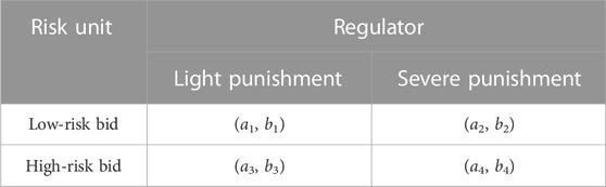
TABLE 1. Payoff matrix for basic risk units and regulator.

Replicator dynamics equations (RDEs) for risk units and the regulator are Eq. (1) and Eq. (2), respectively (Amann and Possajennikov, 2009).

$\frac{d\left(p\right)}{dt}=p\left(1-p\right)\left[q\left(\alpha -\beta \right)+\beta \right],(1)$

$\frac{d\left(q\right)}{dt}=q\left(1-q\right)\left[p\left(\gamma -\delta \right)+\delta \right],(2)$

where 1-p and 1-q are non-negative and have no substantial effect on the evolutionary results of strategy selection. For the sake of discussion, Eq. (1) and Eq. (2) are simplified to the following equations.

$\frac{d\left(p\right)}{dt}=p\left[q\left(\alpha -\beta \right)+\beta \right],(3)$

$\frac{d\left(q\right)}{dt}=q\left[p\left(\gamma -\delta \right)+\delta \right].(4)$

Introducing Gaussian white noise into Eq. (3) and Eq. (4) (Xu et al., 2015), the one-dimensional Itô stochastic replicator dynamic equations (SRDEs) for players are as follows:

$\mathrm{d}p\left(t\right)=p\left(t\right)\left[q\left(t\right)\left(\alpha -\beta \right)+\beta \right]\mathrm{d}\left(t\right)+{\mu }_{1}p\left(t\right)\mathrm{d}\omega \left(t\right),(5)$

$\mathrm{d}q\left(t\right)=q\left(t\right)\left[p\left(t\right)\left(\gamma -\delta \right)+\delta \right]\mathrm{d}\left(t\right)+{\mu }_{2}q\left(t\right)\mathrm{d}\omega \left(t\right),(6)$

where ω(t) is a one-dimensional standard Brownian motion, representing a random fluctuation phenomenon, that effectively reflects how players are affected by stochastic disturbance factors. dω(t) obeys the normal distribution N (0, $\sqrt{h}$). μ₁ and μ₂ represent the intensity of stochastic disturbance. The strategy probabilities at time t for the low-risk bidding and mild punishment are denoted as p(t) and q(t), respectively.

2.2 Existence and stability of trivial solution

By combining the stochastic Taylor expansion and the Itô stochastic formula, the nonlinear Itô SRDE can be expanded and solved with Gaussian random disturbances (Hu et al., 2008).

Considering the following general Itô stochastic differential equation (SDE) (Kamrani, 2015),

$\mathrm{d}x\left(t\right)=f\left(t,x\left(t\right)\right)\mathrm{d}t+g\left(t,x\left(t\right)\right)\mathrm{d}\omega \left(t\right),(7)$

where t∈[t₀,T], x(t₀) = x_0, x₀∈R, h=(T-t₀)/r, and t_s = t₀+sh. r is the number of sampling times, t₀ is the initial time point, and t_s is the sth sampling time point. s∈{0,1,…,r}, performing a stochastic Taylor expansion on Eq. (7), we obtain

$x\left(t_{n+1}\right)=x\left(t_n\right)+J_{0}f\left(x\left(t_n\right)\right)+J_{1}g\left(x\left(t_n\right)\right)+J_{11}{G}^{1}g\left(x\left(t_n\right)\right)+J_{00}{G}^{0}f\left(x\left(t_n\right)\right)+R,(8)$

where J₀ = h, J₁ = ∆ω_n, J₁₁ = [(∆ω_n)²-h]/2, G⁰ = $\partial g\left(x\right)/\partial x+\left(1/2\right){\partial }^{2}g\left(x\right)/\partial x^2$, G¹ = $\partial g\left(x\right)/\partial x$, J₀₀ = h²/2, and R is the remainder term of the expansion.

In practical applications, the Milstein method can be used to numerically iterate and solve the SDE by truncating some terms in the stochastic Taylor expansion (Kai and Guiding, 2022). The format of the Milstein method is as follows:

$x\left(t_{n+1}\right)=x\left(t_n\right)+hf\left(x\left(t_n\right)\right)+\left[{\left(\Delta {\omega }_n\right)}^2-h\right]g\left(x\left(t_n\right)\right)g^{\prime }\left(x\left(t_n\right)\right)/2.(9)$

Based on Eq. (9), the equilibrium solutions for SRDEs Eq. (5) and Eq. (6) can be calculated. The stability analysis of their stochastic evolution is as follows (Hu et al., 2008; Kamrani, 2015):

Given an SDE, suppose there exists a function V(t, x) such that c₁|x|l ≤ V(t, x)≤c₂|x|l, where c₁, c₂, and l are all positive constants. If there exists a positive constant σ such that V*(t, x)≤-σV(t, x), then the l-order moment of the zero-solution of Eq. (7) is said to be exponentially stable, and it holds:

$E{\left|x\left(t,x_0\right)\right|}^l<\left(c2/c1\right){\left|x_0\right|}^l{e^{-}}^{\eta t},t\ge 0,(10)$

$V*\left(t,x\right)=V_t\left(t,x\right)+V_x\left(t,x\right)f\left(t,x\right)+g^2\left(t,x\right)V_{xx}\left(t,x\right)/2.(11)$

According to the aforementioned theorem, for Eq. 5 and Eq. 5, taking V(t, p(t)) = p(t), where p(t)∈(0,1],V(t, q(t)) = q(t), where q(t)∈(0,1], c₁ = c₂ = 1, l = 1, η = 1, then V*(t, p(t)) = f(t, p(t)) = p(t)[q(t)(α-β)+β],V*(t, q(t)) = f(t, q(t)) = q(t)[p(t)(γ-δ)+δ]. If the l-order moment of the zero-solution is stable, it must satisfy the condition that

$p\left(t\right)\left[q\left(t\right)\left(\alpha -\beta \right)+\beta \right]\le -p\left(t\right),(12)$

$q\left(t\right)\left[p\left(t\right)\left(\gamma -\delta \right)+\delta \right]\le -q\left(t\right).(13)$

Subsequently, the proposition of Eq. (12) can be expressed as follows:

C₁, when p(t)∈(0,1], α-β>0, it holds that q(t)≤(-β-1)/(α-β), and α+1 ≥ 0.

C_2, when p(t)∈(0,1], α-β<0, it holds that q(t)≥(-β-1)/(α-β), and α+1 ≤ 0.The conditions to satisfy Eq. (13) are as follows:

C_3, when q(t)∈(0,1], γ-δ>0, it holds that q(t)≤(-δ-1)/(γ-δ), and γ+1 ≥ 0.

C₄, when q(t)∈(0,1], γ-δ<0, it holds that q(t)≥(-δ-1)/(γ-δ), and γ+1 ≤ 0.

The paper randomly sets the value of α, β, γ, and δ, which satisfied the aforementioned propositions C₁ and C₃. Then, the zero-solution exponential stability of Eq. 1–Eq.2 and Eq. 5–Eq. 6 is simulated. The trend in Figure 1 demonstrates the validity of the SEG model and the differences between SEG and CEG models. It is evident that SEG and CEG models show different features. The SEG model can simulate randomness and uncertainty in the real world, whereas the CEG model is more suitable for problems with well-defined strategies and rules. Figure 1A illustrates a more realistic evolutionary path of players’ strategies. In the period of 0 h–39 h, strategy probabilities experience significant fluctuations in the SEG model. The fluctuations better simulate players’ decision-making interfered with by various external or internal factors. By contrast, the CEG path remains smooth, with players evolving undisturbed in an ideal state, as presented in Figure 1B.

FIGURE 1

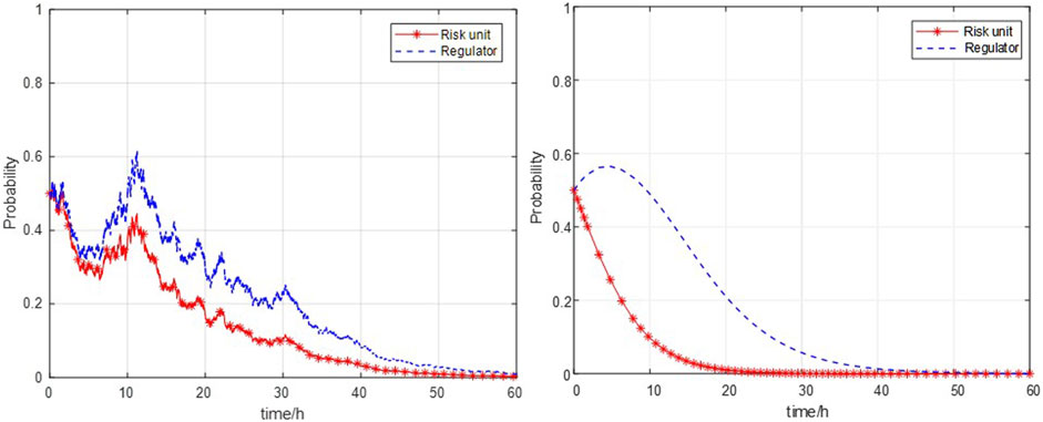
FIGURE 1. Zero-solution exponential stability of games. (A) Stochastic evolutionary game. (B) Classical evolutionary game. Propositions C₁ and C₃: α = −0.04, β = -0.05, γ = 0.08, δ = −0.03, and p_initial = q_initial = 0.5.

3 Stochastic evolutionary game–optimal market-clearing model

Model construction can employ a dual-level optimization method and an adaptive dynamic programming method. The former is more suitable when there are sufficient computational resources and a relatively small state space. It has a simple principle and is convenient for studying the impact of parameter variations within the model. The latter is better suited for problems that are model-independent or have requirements related to data efficiency (Hu et al., 2022; Wang et al., 2022).

A two-layer optimization model incorporating SEG is constructed as the foundation for studying market risk prevention mechanisms. The upper layer represents the SEG which involves the regulator and risk units, while the lower layer displays the optimal market-clearing module, as depicted in Figure 2. The model framework demonstrates the payoffs and strategies of the players in the game, as well as the factors considered when adjusting the evolutionary game strategies.

FIGURE 2

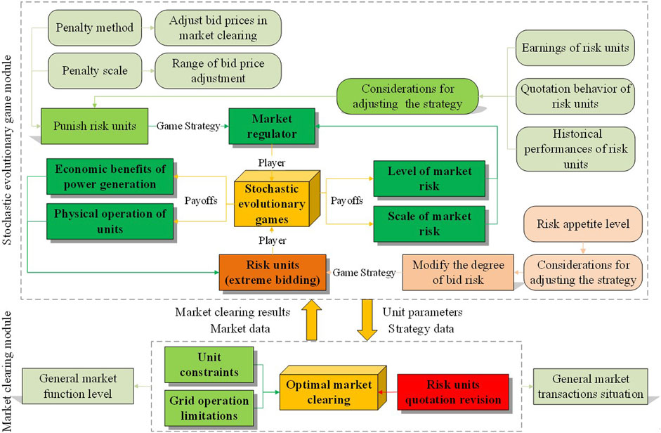
FIGURE 2. Dual-layer iterative model framework.

3.1 SEG model

The pure strategy game matrix of players is shown in Table 2. A_d,i and B_d,i are all positive normalized indicators, which respectively denote the payoffs of each strategy combination on trading day d_i.

TABLE 2

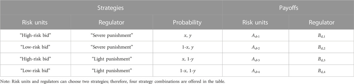
TABLE 2. Pure strategy game matrix for the regulator and the risk group.

(1) Winning rate of the unit

$R_{n,d,t}=\frac{Q_{n,d,t}}{P_{n,d,t}},(14)$

3.1.1 Risk unit payoffs

The formulation of A_d,i primarily takes into account the physical operation and economic revenue aspects of power generation units.

Indicators for the physical operation aspect can be quantified as shown in Eq. (14) and Eq. (15). where Q_n,d,t represents the winning capacity of unit n at time t on trading day d. P_n,d,t represents the declared capacity of unit n at time t on trading day d.

(2) Relative utilization rate of the unit (Reitzes et al., 2007)

Measuring the capacity utilization rate of a unit in market trading, the indicator is calculated as follows:

$R{U}_{n,d,t}=\frac{Q_{n,d,t}}{G_n}·\frac{Q_{d,t}^{eq}}{G_w},(15)$

where G_n is the installed capacity of unit n, $Q_{d,t}^{eq}$ is the system load at time t on trading day d, and G_w is the total installed capacity in the spot market.

The economic dimension indicators are shown in Eq. (16) and Eq. (17).

(1) Expected profit deviation rate

Measuring the difference in the unit’s generation returns for 2 consecutive years, the indicator is calculated as follows:

$D{R}_{n,d,t}=\frac{C{R}_{n,d,t}-L{R}_{n,d,t}}{C{R}_{n,d,t}},(16)$

where CR_n,d,t is the actual profit of unit n at time t on trading day d, while LR_n,d,t represents the actual profit of unit n at the same time slot in the previous year.

(2) Unit sales margin

$M_{n,d,t}=\frac{S_{n,d,t}-C_{n,d,t}}{S_{n,d,t}},(17)$

where C_n,d,t is the generation cost of unit n at time t on trading day d, and S_n,d,t is the income of unit n at time t on trading day d.

Based on sub-indicators from the economic and physical aspects, the income of risk unit n at time t on trading day d, denoted as A_n,d,t, is shown in Eq. (18). Hence, risk units’ payoffs A_d,i are defined by Eq. (19).

$A_{n,d,t}={\theta }_1{R}_{n,d,t}+{\theta }_{2}R{U}_{n,d,t}+{\theta }_3{M}_{n,d,t}+{\theta }_{4}D{R}_{n,d,t},(18)$

$A_{d,i}={\displaystyle \sum _{t=1}^T}\frac{{\displaystyle \sum _{n=1}^N}{A}_{n,d,t}}{R{N}_{d,t}}/T,(19)$

where θ₁–θ₄ are weights of the indicator, RN_d,t is the number of risk units at time t on trading day d, T is the total number of trading periods in 1 day (in this study, it is taken as 24), and N is the total number of power generation units in the power spot market.

3.1.2 Regulator payoffs

B_d,_i considers the market risk level and risk scale. The market risk level is measured by the indicators shown in Eq. 20, Eq. 21

(1) Average relative bidding level (Xie et al., 2023a)

Measuring the extent to which the bid price of a specific unit deviates from the overall average bid price of its peers, the indicator is calculated as follows:

$RL{Q}_{d,t}={\displaystyle \sum _{n=1}^N}\frac{\overline{p_{n,d,t}}-{\displaystyle \sum _{j\ne n}^N}\overline{p_{j,d,t}}/N}{{\displaystyle \sum _{j\ne n}^N}\overline{p_{j,d,t}}/N}/N,(20)$

where $\overline{p_{n,d,t}}$ represents the average bid price of unit n at time t on trading day d.

(2) Degree of proximity of market limit price (Bao et al., 2021)

Measuring how close a power generation unit’s bid price is to the power spot market’s highest price limit, the indicator is calculated as follows:

$L{P}_{d,t}=\frac{{\lambda }_{d,t}}{{\lambda }_l},(21)$

where λ_d,t is the market-clearing price at time t on trading day d and λ_l is the maximum market-clearing price limit.

(3) Proportion of high-risk units to all risk units

Measuring the overall level of the power spot market risk, the indicator is calculated as follows:

$V_{d,t}=\frac{HR{N}_{d,t}}{R{N}_{d,t}},(22)$

where HRN_d,t is the number of high-risk units at time t on trading day d.

The market risk scale measurement indicators are given by Eq. 23.

(1) Proportion of risk units among all units in the market

$D_{d,t}=\frac{R{N}_{d,t}}{N}.(23)$

The income of the regulator at time t on trading day d, denoted as B_d,t, is derived from the sub-indicators related to market risk level and scale, as shown in Eq. (24). So the regulator’s payoffs B_d,i is defined by Eq. (25).

$B_{d,t}={\omega }_1{V}_{d,t}^{\prime }+{\omega }_2{D}_{d,t}^{\prime }+{\omega }_{3}RL{Q}_{d,t}^{\prime }+{\omega }_{4}L{P}_{d,t}^{\prime },(24)$

$B_{d,i}={\displaystyle \sum _{t=1}^T}{B}_{d,t}/T,(25)$

where ω₁–ω₄ are the weights of the indicator. $V_{d,t}^{\prime }$ is indicator V_d,t after being positive normalized. The remaining indicators follow the same processing approach.

3.2 Optimal market-clearing model

The optimal market-clearing model implements the paper’s risk prevention mechanism by increasing the bid prices of risk units during market clearing, which uses market-based measures to constrain the winning capacity of risk units rapidly and accurately. Our earlier work on this model is detailed in Xie et al. (2023a). In this paper, the optimal market-clearing model is used as the same as our previous work.

3.3 Computational process of the total model

The “stochastic evolutionary game–optimal market-clearing” model follows a top–down iterative process, as depicted in Figure 3. The specific steps are as follows.

(1) On trading day d_i, the equilibrium stability analysis is conducted through the SEG model to determine a stable equilibrium point (x, y) and the stochastic evolutionary stabilization strategy (SESS) of players. Then, the risk unit group’s SESS and the regulator’s SESS will be outputted. Additionally, data regarding four strategy combinations of players are computed.

(2) Four sets of strategy data are separately fed into the optimal market-clearing algorithm. This algorithm facilitates a unified clearing process for both risk units and non-risk units in every strategy combination of players, resulting in the determination of winning capacities of units and market-clearing prices for four strategy combinations.

(3) Based on the power market operation and clearing data, the payoffs of players in the game can be calculated. Then, the payoff matrix for the SEG model is updated.

(4) Another round of SEG stability analysis is performed to obtain SESS for the next trading day d_i+1. The data for each strategy combination are calculated. Finally, one iteration of the SEG model on trading day d_i is completed.

FIGURE 3

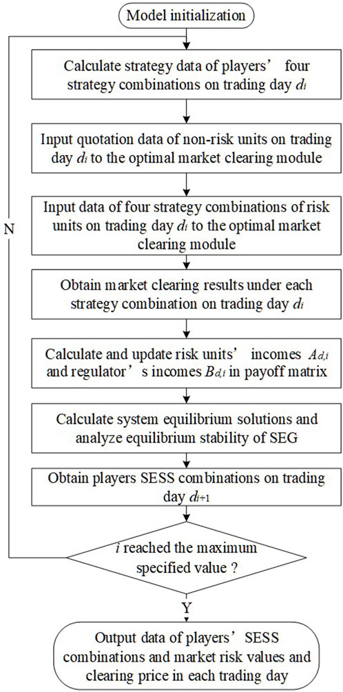
FIGURE 3. Model iterative calculation flow chart.

4 Quantitative strategies for players

4.1 Regulator strategy development

In the market-clearing process, risk units are subject to bid price adjustments based on their risk levels. It aims to reduce their winning capacity as a form of “penalty.” Penalties are positively correlated with the magnitude of bid price revisions. The development of the regulator’s risk prevention strategy considers both subjective and objective factors.

When considering objective factors in the power spot market, several indicators are formulated based on the aspect of risk units’ power generation incomes, risk units’ historical performances, and risk units’ bidding behaviors.

4.1.1 Indicators for measuring the risk unit’s power generation incomes

Indicators measuring risk units’ power generation incomes are defined in Eq. 26–Eq. 29.

(1) Deviation degree of risk unit electricity price

We measure the extent to which the market-clearing price of a risk unit deviates from the average market-clearing price of comparable units. Its formula is as follows.

$D{P}_{n,d}={\displaystyle \sum _{t=1}^T}\frac{{\lambda }_{n,d,t}^r-\overline{{\lambda }_{n,d,t}^c}}{\overline{{\lambda }_{n,d,t}^c}}/T,(26)$

where ${\lambda }_{n,d,t}^r$ is the market-clearing price of risk unit n at time t on trading day d. $\overline{{\lambda }_{n,d,t}^c}$ is the average market-clearing price of normal units (the same cost-type as risk unit n) at time t on trading day d.

(2) Risk unit income deviation

We measure the extent to which the income of a risk unit deviates from the average income of comparable units. Its formula is as follows.

$D{S}_{n,d}={\displaystyle \sum _{t=1}^T}\frac{S_{n,d,t}^r-\overline{S_{n,d,t}^c}}{\overline{S_{n,d,t}^c}}/T,(27)$

where $S_{n,d,t}^r$ is the income of risk unit n at time t on trading day d. $\overline{S_{n,d,t}^c}$ is the average income of normal units (the same cost-type as risk unit n) at time t on trading day d.

(3) High-price winning rate of the risk unit (Wang et al., 2022)

The formula for calculating the proportion of winning capacity at the high bid price for a risk unit can be expressed as follows.

$W{R}_{n,d}^h={\displaystyle \sum _{t=1}^T}\frac{Q_{n,d,t}^h}{q_{n,d,t}^h}/T,(28)$

where $Q_{n,d,t}^h$ is the winning capacity of risk unit n at time t on trading day d, which bids at a high price. $q_{n,d,t}^h$ is the high price declared capacity of risk unit n at time t on trading day d.

(4) Actual markup index of the risk unit (Han et al., 2023)

The method for measuring the extent to which the market-clearing price deviates from the marginal cost of the unit’s generation is as follows:

$PA{I}_{n,d}={\displaystyle \sum _{t=1}^T}\frac{{\lambda }_{n,d,t}^r-C_{n,d,t}^{ac}}{C_{n,d,t}^{ac}}/T,(29)$

where $C_{n,d,t}^{ac}$ is the generation cost of risk unit n at time t on trading day d.

To obtain the overall indicator $I_{{\text{RUGR}}_{n,d}}$ for measuring the generation income of risk units in risk prevention strategies, the weighted sum of the sub-indicators can be calculated.

$I_{RUG{R}_{n,d}}={\eta }_{1}D{P}_{n,d}+{\eta }_{2}D{S}_{n,d}+{\eta }_{3}W{R}_{n,d}^h+{\eta }_{4}PA{I}_{n,d},(30)$

where η₁–η₄ are weights of sub-indicators.

4.1.2 Methods for evaluating the risk unit’s historical performances

The historical performance aspect includes indicators such as historical anomaly level and credit rating.

(1) Risk unit historical anomaly level

The historical anomaly level can be determined by counting the number of times a unit has been identified as a risk unit in the past.

(2) Risk unit credit rating

The credit rating of a unit can be determined by assessing the overall creditworthiness of the power generation company to which the unit belongs.

4.1.3 Indicators for the risk unit’s bidding behaviors

Indicators measuring bidding behaviors are as follows.

(1) Maximum bid price differential index of the risk unit (Han et al., 2023)

Assess behaviors of risk units that allocate a significant portion of their capacity to low-bidding segments to ensure winning bids, while allocating a smaller portion of their capacity to high-bidding segments, thereby elevating the market-clearing price.

$M{D}_{n,d}^{\max }=\left\{\begin{array}{l}1,{\max }_{1\le k\le K-1}\left\{p_{n,d,t,k+1}^r-p_{n,d,t,k}^r\right\}\ge \delta \left(p_{\max }-p_{\min }\right)\\ 0,else\end{array}\right.,(31)$

where $p_{n,d,t,k}^r$ and $q_{n,d,t,k}^r$ represent the bid price and bid capacity of risk unit n at time t on trading day d in the kth bidding segment, respectively. p_max and p_min represent the maximum and minimum bid prices specified by the market, respectively, while δ denotes the allowed bid price differential range.

(2) Relative bidding level of the risk unit

It is followed Eq. (20).

(3) Risk unit bidding premium index (Chen et al., 2018)

The index measures the proportion by which unit bids deviate from their marginal costs.

$BA{I}_{n,d}^r={\displaystyle \sum _{t=1}^T}\frac{\overline{p_{n,d,t}^r}-C_{n,d}^{ac}}{C_{n,d}^{ac}}/T.(32)$

The total indicator $I_{{\text{RUOB}}_{n,d}}$ for measuring bidding behaviors of risk units is obtained by weighting and summing up the sub-indicators.

$I_{RUO{B}_{n,d}}={\pi }_{1}M{D}_{n,d}^{\max }+{\pi }_{2}RL{Q}_{n,d}^r+{\pi }_{3}BA{I}_{n,d}^r,(33)$

where π₁–π₃ are weights of the sub-indicators.

4.1.4 Strategy formulation for the regulator

Based on the assumption of bounded rationality of players in the evolutionary game, the subjective influence of the regulator’s willingness to adjust bid prices of risk units is measured by probabilities {y, 1-y}. The greater the probabilities y or 1-y, the higher the regulator’s willingness to choose a strong or light punishment strategy and vice versa (Xie et al., 2021). In brief, the regulator’s strategy, considering both objective market factors and subjective punishment willingness, can be represented by Eq. (34). The bidding adjustment function for risk units is defined as follows:

$p_{t,n}^{\prime }=p_{t,n}\left(1+\tau \right),(34)$

where $p_{t,n}^{\prime }$ is the adjusted bid price of the risk unit, p_n,t is the original bid price of the risk unit n, and τ represents the degree of bid adjustment.τ₁ represents the regulator’s strong punishment strategy. τ₂ represents the regulator’s light punishment strategy. They are determined as shown in Eq. (35) and Eq. (36), respectively.

${\tau }_1={\tau }_0·\left({\mu }_1{C}_1+{\mu }_2{C}_2\right)·S_1\left(y\right),(35)$

${\tau }_2={\tau }_0·\left({\mu }_1{C}_1+{\mu }_2{C}_2\right)·S_2\left(y\right),(36)$

where τ₀ is the given initial value of τ. C₁ and C₂ are objective factors for the strategy based on the risk unit’s generation income, bidding behavior, and historical performance. μ₁ and μ₂ represent the weights of C₁ and C₂, respectively. S₁(y) and S₂(y) are subjective modifying factors for the regulator’s penalty strategy based on its subjective punishment willingness. The values of C₁, C₂, and S₁(y), S₂(y) can be found in Section 5.1.

4.2 Strategy formulas of risk units

The electricity market has been shown to involve both renewable and conventional energy units in this paper. Compared to conventional energy units, renewable energy units have a distributed nature. It imposes requirements on units’ output stability and regulatory capabilities. In this paper, it can be approximated that their game strategy selection and formulation are assumed to be identical.

Risk units adjust bid strategies based on their own benchmark prices. Risk units, being the group with bounded rationality and asymmetric information compared to the regulator, rely more on subjective risk preferences when formulating a bid strategy (Jiao et al., 2017). Specifically, the high-risk bid strategy and low-risk bid strategy are defined as shown in Eq. (37) and Eq. 38, respectively:

$p_{t,n}^h=p_{t,n}^b{S}_1\left(x\right),(37)$

$p_{t,n}^l=p_{t,n}^b{S}_2\left(x\right),(38)$

where S₁(x) and S₂(x) are risk-modifying factors that represent the subjective risk preference of risk units. $p_{t,n}^b$ represents the benchmark bid price for risk unit n at time t. According to reports of China’s National Development and Reform Commission (National Development and Reform Commission, 2021a; National Development and Reform Commission, 2021b), the range of risk bid price is defined as a 20% fluctuation around the benchmark price. The values of S₁(x) and S₂(x) can be found in Section 5.1.

5 Case study

The data used for our analysis consist of the trial operation data from the power spot market in a specific region of East China for a continuous period of 10 trading days (d₁–d₁₀). The market information is shown in Figure 4. A total of 54 power generation units participate in the spot market. Among them, thermal power units are numbered from 1 to 25, while renewable energy units are numbered from 26 to 54.

FIGURE 4

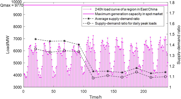
FIGURE 4. Electricity load curves and market supply–demand ratios for 240 h time periods in a region of East China.

Our earlier work on the power generation units’ risk identification method is detailed in Xie et al. (2023b). It allows for the risk detection of 54 units. The risk behavior exhibited by identified risk units during trading days d₁–d₄ is intentional withholding, while during trading days d₅–d₁₀, it involves extremely high offers.

5.1 Preparation for model simulation

To calculate the strategy data for players in the SEG, it is necessary to establish data fuzzy classification rules. Additionally, strategy modifying factors C₁, C₂, S₁(y), and S₂(y) and risk preference factors S₁(x) and S₂(x) need to be determined.

The fuzzy classification rules for probability and indicator data are as follows.

(1) Strategy selection probabilities

Probabilities {x, y, 1-x, 1-y} are divided into four classes, as shown in Table 3.

TABLE 3

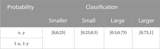
TABLE 3. Classification of strategy selection probabilities.

(2) Indicator data

According to market trading results, the upper, middle, and lower quartiles, j_i, g_i, and e_i, are chosen to classify $I_{{\text{RUGR}}_{n,d}}$ and $I_{{\text{RUOB}}_{n,d}}$ in a fuzzy manner. See Table 4 and Table 5.

TABLE 4

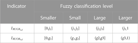
TABLE 4. Fuzzy classification of indicators in terms of generation income and bidding behavior of risk units.

TABLE 5

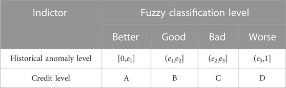
TABLE 5. Fuzzy classification of indicators in terms of historical performance of risk units.

The membership functions for the modifying factors C₁ and C₂ can be represented by Eq. (50) and Eq. 51, respectively.

$C_1={\phi }_1\exp \left(p_1+p_2\right)+{\nu }_1,(50)$

$C_2={\phi }_2/\left(q_1+q_2\right)+{\nu }_2.(51)$

When $I_{{\text{RUGR}}_{n,d}}$ is smaller, small, large, and larger, p₁ can be taken as 1, 2, 3, and 4, respectively, and the same relationship exists with $I_{{\text{RUOB}}_{n,d}}$ and p₂. When the historical anomaly level is better, good, bad, and worse, q₁ can be taken as 1, 2, 3, and 4, respectively, and the same relationship exists between credit level and q₂. φ₁, ν₁, φ₂, and ν₂ that are coefficients to be determined.

S₁(y) and S₂(y) are determined by values of τ, C₁, and C₂. They are divided into four parts equally, each forming a membership function with probabilities y and 1-y, respectively, as shown in Table 6.

TABLE 6

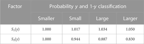
TABLE 6. Values of modification factors S₁(y) and S₂(y).

S₁(x) and S₂(x) are determined by the upper and lower limits of risk units’ bid price. They are divided into four parts equally, each forming a membership function with probabilities x and 1-x, respectively, as shown in Table 7.

TABLE 7

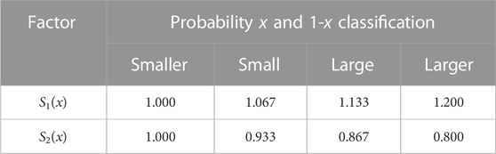
TABLE 7. Values of correction factors S₁(x) and S₂(x).

5.2 Analysis of the stochastic evolutionary dynamics of players’ strategies

Once the set of risk units is determined, a simulation analysis can be performed using the MATLAB platform. The initial strategy selection probabilities are set as x(0) = 0.7 and y(0) = 0.6. The initial time is t₀ = 0, and the number of samples, r, is set to 1,500. The simulation time, T, is 240 h. The random disturbance intensity index, a, is taken as 0, 1, or 2. In this section, a detailed analysis of the evolutionary dynamics will be conducted specifically for trading day d₁. The analysis principles for the remaining trading days (d₂ to d₁₀) are the same and will not be reiterated. The detailed analysis for trading day d₁ is as follows.

1. Because of the random disturbance, the evolutionary game system exhibits fluctuations as it converges to the equilibrium point, as is shown in Figure 5. Finally, the combination of players’ SESS is the risk units’ low-risk bid and the regulator’s light punishment.

2. Under different disturbance intensities, the regulator reaches its equilibrium strategy in approximately the same time, which is 14 h. On the other hand, the risk units reach the equilibrium strategy in 24 h, 19.5 h, and 17.8 h for intensity coefficient a = 0, 1, and 2, respectively. This indicates that the random disturbance factor accelerates the evolutionary pace of risk units, and the evolutionary rate is positively correlated with the intensity of the system disturbance.

3. The high intensity of random disturbance amplifies the probability fluctuations during the evolutionary processes. Taking time t = 2 as an example, probabilities and their variations under different disturbance intensities are shown in Table 8. For risk units, during the initial stage of system evolution (t = 0 to t = 8), the probability x(t) shows a significant decline, followed by a local rebound. It suggests that the willingness of the risk unit group to adopt compliant bid behaviors and avoid penalties has rapidly increased when they were punished by the regulator.

FIGURE 5

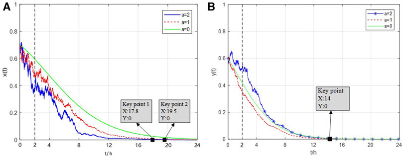
FIGURE 5. Evolutionary paths of players on trading day d₁ under the stochastic disturbance system. (A) Evolutionary path of the strategy of risky units under stochastic disturbance intensity coefficient a = 2, 1, and 0. (B) Evolutionary path of the strategy of the regulator under stochastic disturbance intensity coefficient a = 2, 1, and 0.

TABLE 8

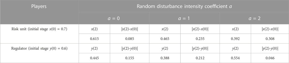
TABLE 8. Fluctuation amplitude of strategy probabilities under different stochastic disturbance intensities at time t = 2 on trading day d₁.

Due to random factors such as risk awareness or risk preference, the strategy probabilities of the risk group fluctuate, and the fluctuation increases with a stronger disturbance. It is evident that various factors, including risk awareness and risk preference, introduce randomness into the strategy probabilities of risk groups. Moreover, this randomness becomes more pronounced with increasing external disturbances. As the game unfolds, risk units tend to gravitate toward stable, low-risk bidding strategies in order to safeguard their baseline incomes. From the regulatory standpoint, decision-making is influenced by stochastic elements such as market-clearing outcomes, appeals, and public sentiment. When the level of random disruption intensifies, regulatory decisions exhibit more substantial fluctuations in the initial stages of evolution.

When applying the combination of a low-risk bid and light punishment strategy, the market risk level decreases and the overall market environment tends to stabilize. Therefore, there is no significant fluctuation in the evolution path of players on trading days d₂ and d₃, as shown in Figure 6.

FIGURE 6

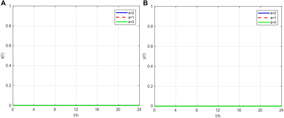
FIGURE 6. Evolutionary paths of players on trading days d₂, d₃, and d₇–d₁₀ under the stochastic disturbance system. (A) Evolutionary path of the strategy of risky units under stochastic disturbance intensity coefficient a = 2, 1, and 0. (B) Evolutionary path of the strategy of the regulator under stochastic disturbance intensity coefficient a = 2, 1, and 0.

It is worth noting that the tight electricity supply–demand on trading days d₅ to d₁₀ creates the willingness for risk units to increase their risk level. The risk behavior also shifts from intentional withholding to extremely high offers. As is shown in Figure 7, on trading day d₄, there is a change in the evolutionary process due to the decrease in the supply–demand ratio. This indicates that even with the implementation of risk prevention strategies, there is still a motivation for risk units to increase their bid risk level in the game with the regulator. There is a lag in the decision-making process of the regulatory authority.

FIGURE 7

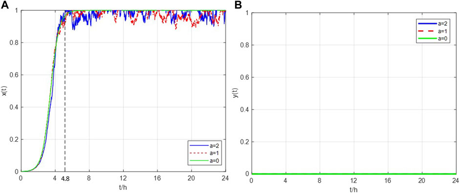
FIGURE 7. Evolutionary paths of players on trading day d₄ under the stochastic disturbance system. (A) Evolutionary path of the strategy of risky units under stochastic disturbance intensity coefficient a = 2, 1, and 0. (B) Evolutionary path of the strategy of the regulator under stochastic disturbance intensity coefficient a = 2, 1, and 0.

The evolutionary process of trading day d₅ is depicted in Figure 8. The light punishment strategy appears to have insufficient deterrence on the risk group, resulting in risk units continuing to adopt a high-risk bid strategy. Consequently, the regulator experiences a decline in its income, leading to a shift back to the strong penalty strategy.

FIGURE 8

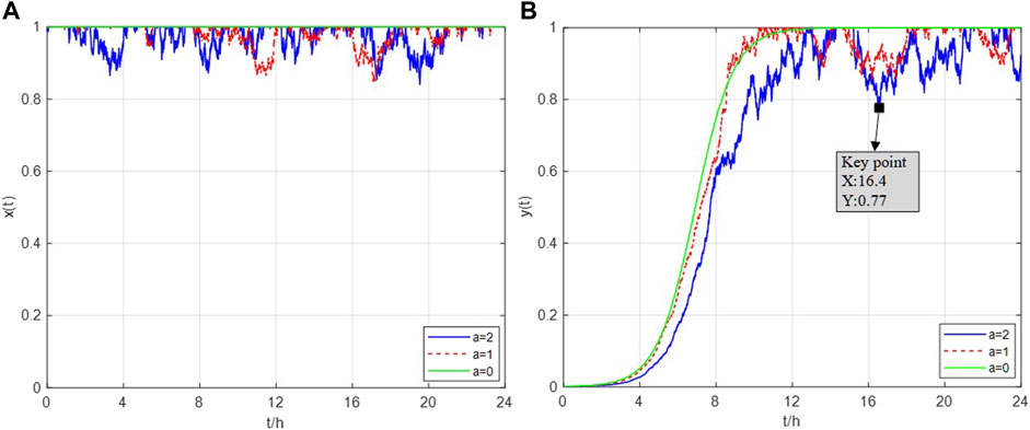
FIGURE 8. Evolutionary paths of players on trading day d₅ under the stochastic disturbance system. (A) Evolutionary path of the strategy of risky units under stochastic disturbance intensity coefficient a = 2, 1, and 0. (B) Evolutionary path of the strategy of the regulator under stochastic disturbance intensity coefficient a = 2, 1, and 0.

The evolutionary paths shown in Figure 9 illustrates that risk units rapidly change to a low-risk bid strategy on trading day d₆ due to the regulator’s imposition of strong penalties. In contrast, the regulator’s strategy evolves at a slower pace, indicating concerns about the possibility of risk units reverting to a high-risk bid behavior. Random disturbances accelerate the evolution time for players with a maximum reduction of over 12 h when the intensity coefficient a is set to 2.

FIGURE 9

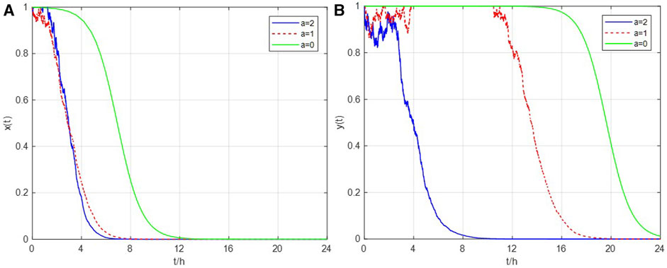
FIGURE 9. Evolutionary paths of players on trading day d₆ under the stochastic disturbance system. (A) Evolutionary path of the strategy of risky units under stochastic disturbance intensity coefficient a = 2, 1, and 0. (B) Evolutionary path of the strategy of the regulator under stochastic disturbance intensity coefficient a = 2, 1, and 0.

After the SEG of multiple trading days, the regulatory mechanism has successfully suppressed the willingness of risk units to increase their bid risk. Meanwhile, in an effort to minimize administrative intervention in the power market, the regulator has maintained a light punishment strategy. As a result, the market operation has entered a virtuous cycle. The evolutionary paths of players on trading days d₇ to d₁₀ are depicted in Figure 6.

5.3 Analysis of spot market trading and operational risk prevention

Due to penalties imposed by the regulator, the winning capacities of risk units on each day have decreased. Among them, the decrease in the awarded capacities of thermal power units is significantly greater than those of renewable energy units, as detailed in Table 10. The observed phenomenon can be attributed to the following reasons: Thermal power units typically have higher declared capacities and are more sensitive to changes in prices compared to renewable energy units. Therefore, the impact of different bid risk levels on winning capacities of thermal power units is much greater than that of renewable energy units.

Obviously, with the increase in the level of bid risk or the intensity of punishments, the decline rate of risk units’ winning capacities becomes larger. Table 9 presents changing rates of winning capacities for different SESS between the regulator and risk units, highlighting this effect. In more extreme market conditions, where players adopt a strategy combination of severe punishment and a high-risk bid, the average change rate for risk units approaches 50%. When players adopt a combination of the mild penalty and low-bidding risk strategy in milder market environments, this value does not exceed 14%.

TABLE 9

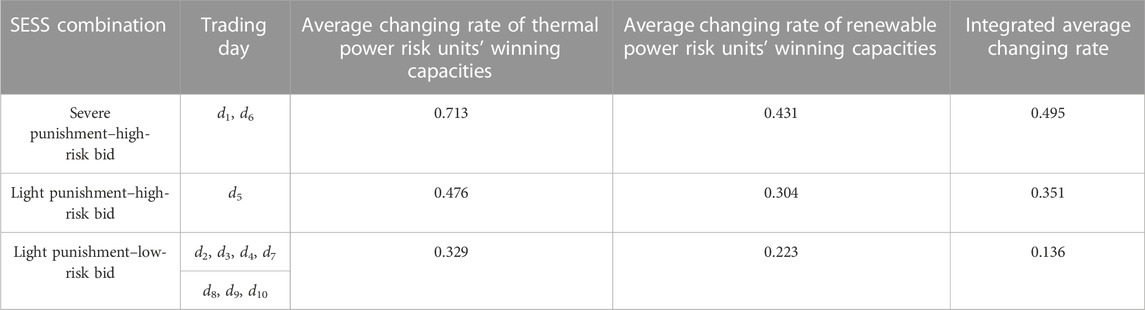
TABLE 9. Change rates of winning capacities for different types of risk units under different SESS combinations.

After the regulator has imposed penalties on risk units, regardless of the strength of punishment, the average market-clearing price has been found to decrease. The maximum decrease has reached 156.9 yuan/MWh, with a maximum change rate of 17.3%.

Given the constrained supply–demand conditions on trading days d₅–d₁₀, the reduction in electricity prices during this period is less pronounced compared to days d₁ to d₄, when supply and demand are more balanced. When comparing the average electricity price decrease of 139.1 yuan/MWh and an average price volatility of 17.2% during trading days d₁ to d₄, a slightly lower average decrease can be found during trading days d₅ to d₁₀, i.e., 98.5 yuan/MWh, accompanied by an average volatility of 9.8%. It is evident that the prevailing supply and demand conditions significantly influence the effectiveness of the risk prevention mechanism in the spot market, with more favorable risk prevention outcomes observed during periods of lesser supply and demand. The specific situation of market power risk prevention is shown in Table 10.

TABLE 10

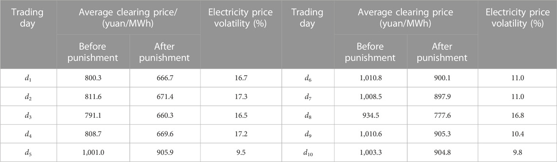
TABLE 10. Situation of power spot market trading risk prevention.

In summary, through the proposed risk prevention mechanism on the generation side of the electricity spot market, market risks brought by market power are effectively mitigated. Price guidance is achieved, which leads to lower trading prices and further improvements in social welfare in electricity transactions.

6 Conclusion

For the emerging power spot market in China, it is crucial to ensure its ability to discover the true price of electricity. In this regard, a reasonable and effective market risk prevention mechanism plays a key role. Hence, the basic evolutionary game methodology has been expanded, and a stochastic disturbance factor in the mathematical model, constructing the SEG model, has been introduced. Based on the real power spot market, an adaptive quantitative risk prevention mechanism for extreme bid market power on the supply side of the market is developed. Furthermore, a dual-layer dynamic “stochastic evolutionary game–optimal market-clearing” model is constructed for quantitative analysis.

Data availability statement

The original contributions presented in the study are included in the article/Supplementary Material; further inquiries can be directed to the corresponding author.

Author contributions

JX: conceptualization, funding acquisition, methodology, project administration, resources, supervision, and validation. BG: data curation, formal analysis, investigation, methodology, software, supervision, writing–original draft, and writing–review and editing. YY: conceptualization, methodology, supervision, and writing–review and editing. RL: writing–review and editing. QS: writing–review and editing.

Funding

The author(s) declare financial support was received for the research, authorship, and/or publication of this article. This research was supported by grants from the National Natural Science Foundation of China (U2066214).

Conflict of interest

The authors declare that the research was conducted in the absence of any commercial or financial relationships that could be construed as a potential conflict of interest.

Publisher’s note

All claims expressed in this article are solely those of the authors and do not necessarily represent those of their affiliated organizations, or those of the publisher, the editors, and the reviewers. Any product that may be evaluated in this article, or claim that may be made by its manufacturer, is not guaranteed or endorsed by the publisher.

References

Amann, E., and Possajennikov, A. (2009). On the stability of evolutionary dynamics in games with incomplete information. Math. Soc. Sci. 58, 310–321. doi:10.1016/j.mathsocsci.2009.08.001

CrossRef Full Text | Google Scholar

Amundsen, E. S., and Bergman, L. (2006). Why has the Nordic electricity market worked so well? Util. Policy 14 (3), 148–157. doi:10.1016/j.jup.2006.01.001

CrossRef Full Text | Google Scholar

Bao, M., Ding, Y., Zhou, X., Guo, C., and Shao, C. (2021). Risk assessment and management of electricity markets: a review with suggestions. CSEE J. Power Energy Syst. 7 (6), 1322–1333. doi:10.17775/CSEEJPES.2020.04250

CrossRef Full Text | Google Scholar

Bask, M., Lundgren, J., and Rudholm, N. (2011). Market power in the expanding Nordic power market. Appl. Econ. 43 (9), 1035–1043. doi:10.1080/00036840802600269

CrossRef Full Text | Google Scholar

Bose, S., Wu, C., Xu, Y., Wierman, , and Mohsenian-Rad, H. (2015). A unifying market power measure for deregulated transmission-constrained electricity markets. IEEE Trans. Power Syst. 30 (5), 2338–2348. doi:10.1109/TPWRS.2014.2360216

CrossRef Full Text | Google Scholar

Chen, Q., Yang, J., Huang, Y., Lu, E., and Wang, Y. (2018). Review of market power monitoring and mitigation mechanisms in foreign electricity markets. South. Power Grid Technol. 12 (12), 9–15. doi:10.13648/j.cnki.issn1674-0629.2018.12.002

CrossRef Full Text | Google Scholar

Cheng, L., and Yu, T. (2018). Analysis of equilibrium stability in typical scenarios of multi-group asymmetric evolutionary game in the open power market environment. Proc. Chin. Soc. Electr. Eng. 38 (19), 5687–5703. doi:10.13334/j.0258-8013.pcsee.172219

CrossRef Full Text | Google Scholar

Dagoumas, A. S., Koltsaklis, N. E., and Panapakidis, L. P. (2017). An integrated model for risk management in electricity trade. Energy 124, 350–363. doi:10.1016/j.energy.2017.02.064

CrossRef Full Text | Google Scholar

He, S., He, X., Lou, S., Li, Z., Chen, Z., Gu, H., et al. (2023). Key monitoring indicators and market power analysis of the trial operation of the southern (starting from guangdong) electricity spot market "monthly settlement. Power Syst. Technol. 47 (01), 175–185. doi:10.13335/j.1000-3673.pst.2022.0776

CrossRef Full Text | Google Scholar

Hellmer, S., and Wårell, L. (2009). On the evaluation of market power and market dominance—the Nordic electricity market. Energy Policy 37 (8), 3235–3241. doi:10.1016/j.enpol.2009.04.014

CrossRef Full Text | Google Scholar

Hu, S., Huang, C., and Wu, F. (2008). Stochastic differential equations. Beijing, China: Science Press.

Google Scholar

Hu, X., Zhang, H., Ma, D., Wang, R., and Tu, P. (2022). Small leak location for intelligent pipeline system via action-dependent heuristic dynamic programming. IEEE Trans. Ind. Electron. 69, 11723–11732. doi:10.1109/TIE.2021.3127016

CrossRef Full Text | Google Scholar

Jiao, J., Chen, J., Li, L., and Li, F. (2017). Analysis of local government and enterprise behavior evolutionary game under carbon emission reduction incentive mechanism. Chin. J. Manag. Sci. 25 (10), 140–150. doi:10.16381/j.cnki.issn1003-207x.2017.10.015

CrossRef Full Text | Google Scholar

Kai, L., and Guiding, G. (2022). A family of fully implicit strong Itô-Taylor numerical methods for stochastic differential equations. J. Comput. Appl. Math. 406, 113924. doi:10.1016/j.cam.2021.113924

CrossRef Full Text | Google Scholar

Kamrani, M. (2015). Numerical solution of stochastic fractional differential equations. Numer. Algorithms 68 (1), 81–93. doi:10.1007/s11075-014-9839-7

CrossRef Full Text | Google Scholar

Li, J., Ren, H., and Wang, M. (2021). How to escape the dilemma of charging infrastructure construction? A multi-sectorial stochastic evolutionary game model. Energy 231, 120807. doi:10.1016/j.energy.2021.120807

CrossRef Full Text | Google Scholar

May, R. M., Levin, S. A., and Sugihara, G. (2008). Ecology for bankers. Nature 451 (7181), 893–894. doi:10.1038/451893a

PubMed Abstract | CrossRef Full Text | Google Scholar

National Development and Reform Commission (2021a). Notice on further deepening the market-oriented reform of coal-fired power generation on-grid tariffs. http://www.gov.cn/zhengce/zhengceku/2021/10/12/content_5642159.htm.

Google Scholar

National Development and Reform Commission (2021b). Notice on relevant matters of new energy on-grid electricity price policy in 2021. http://www.gov.cn/zhengce/zhengceku/2021-06/11/cont.

Google Scholar

Rahimi, F., and Sheffrin, A. Y. (2003). Effective market monitoring in deregulated electricity markets. IEEE Trans. Power Syst. 18 (2), 486–493. doi:10.1109/TPWRS.2003.810680

CrossRef Full Text | Google Scholar

Reitzes, J. D., Pfeifenberger, J. P., Fox-Penner, P., Basheda, G. N., and Schumacher, A. C. (2007). Review of PJM‘s market power mitigation practices in comparison to other organized electricity markets. Boston, Massachusetts, USA: The Brattle Group, Inc.

Google Scholar

Shafie-Khah, M., Moghaddam, M. P., and Sheikh-El-Eslami, M. K. (2016). Ex-ante evaluation and optimal mitigation of market power in electricity markets including renewable energy resources. IET Generation Transm. Distribution 10 (8), 1842–1852. doi:10.1049/iet-gtd.2015.0981

CrossRef Full Text | Google Scholar

Shu, J., Han, X., Han, B., and Li, L. (2019). Grid planning considering market force mitigation in electricity market. Power Grid Technol. 43 (10), 3616–3621. doi:10.13335/j.1000-3673.pst.2018.2731

CrossRef Full Text | Google Scholar

Song, Y., Bao, M., Ding, Y., Shao, C., and Shang, N. (2020). Overview of key points for the construction of China’s electricity spot market under the new power reform and relevant recommendations. Proc. Chin. Soc. Electr. Eng. 40 (10), 3172–3187. doi:10.13334/j.0258-8013.pcsee.191251

CrossRef Full Text | Google Scholar

Sun, Q., Yang, Y., Tian, L., Ji, T., Sheng, J., and Xie, Y. (2020). Practice and theoretical exploration of credit limit evaluation for participants in guangdong power spot market. Price Theory Pract. (05), 102–105. doi:10.19851/j.cnki.CN11-1010/F.2020.05.152

CrossRef Full Text | Google Scholar

Wang, R., Ma, D., Li, M., Sun, Q., Zhang, H., and Wang, P. (2022). Accurate current sharing and voltage regulation in hybrid wind/solar systems: an adaptive dynamic programming approach. IEEE Trans. Consumer Electron. 68 (3), 261–272. doi:10.1109/TCE.2022.3181105

CrossRef Full Text | Google Scholar

Wang, R., Sun, Q., Hu, W., Li, Y., Ma, D., and Wang, P. (2021a). SoC-based droop coefficients stability region analysis of the battery for stand-alone supply systems with constant power loads. IEEE Trans. Power Electr. 36, 7866–7879. doi:10.1109/tpel.2021.3049241

CrossRef Full Text | Google Scholar

Wang, R., Sun, Q., Hu, W., Xiao, J., Zhang, H., and Wang, P. (2021b). Stability-oriented droop coefficients region identification for inverters within weak grid: an impedance-based approach. IEEE Trans. Syst. Man. Cybern. Syst. 51 (4), 2258–2268. doi:10.1109/TSMC.2020.3034243

CrossRef Full Text | Google Scholar

Xie, J., Liu, S., Sun, X., Deng, H., and Jiang, H. (2023a). Power market clearing mechanism considering market power risk prevention. Power Constr. 44 (04), 18–28. doi:10.12204/j.issn.1000-7229.2023.04.003

CrossRef Full Text | Google Scholar

Xie, J., Lu, H., Lu, C., and Zhu, S. (2022). Typical foreign electricity market regulation models and their implications for China. J. Electr. Eng. 17 (04), 233–239. doi:10.11985/2022.04.024

CrossRef Full Text | Google Scholar

Xie, J., Lu, S., and Huang, X. (2023b). Analysis of electricity market power risk characteristics and research on identification techniques for adapting to the new power system. Electr. Meas. Instrum., 1–11.

Google Scholar

Xie, J., Wang, S., Zhou, X., Sun, B., and Sun, X. (2021). Regulation strategies in electricity markets based on tripartite evolutionary game. Sci. Technol. Eng. 21 (35), 15072–15083. doi:10.3969/j.issn.1671-1815.2021.35.026

CrossRef Full Text | Google Scholar

Xu, Y., Yu, B., Wang, Y., and Chen, Y. (2015). A stochastic evolutionary game perspective on the stability of strategic alliances against external opportunism. J. Syst. Sci. Complex 28, 978–996. doi:10.1007/s11424-015-2104-x

CrossRef Full Text | Google Scholar

Zhang, W., Yu, J., and Ma, H. (2021). A review of market power mitigation measures in the North American electricity market. Guangdong Electr. Power (04), 24–33. doi:10.3969/j.issn.1007-290X.2021.004.004

CrossRef Full Text | Google Scholar

Zhang, X., and Shi, L. (2020). Research directions and key technologies for the future of China’s power market. Automation Electr. Power Syst. 44 (16), 1–11. doi:10.7500/AEPS20200602001

CrossRef Full Text | Google Scholar

Zhang, Y., Duan, G., Yu, J., Wang, H., Zhang, Z., and Niu, D. (2018). Research on credit evaluation of power sales companies based on KPCA-MEE. Electr. Power 51 (7), 128–135. doi:10.11930/j.issn.1004-9649.201711287

CrossRef Full Text | Google Scholar