Combination optimization method of grid sections based on deep reinforcement learning with accelerated convergence speed

A modern power system integrates more and more new energy and uses a large number of power electronic equipment, which makes it face more challenges in online optimization and real-time control. Deep reinforcement learning (DRL) has the ability of processing big data and high-dimensional features, as well as the ability of independently learning and optimizing decision-making in complex environments. This paper explores a DRL-based online combination optimization method of grid sections for a large complex power system. In order to improve the convergence speed of the model, it proposes to discretize the output action of the unit and simplify the action space. It also designs a reinforcement learning loss function with strong constraints to further improve the convergence speed of the model and facilitate the algorithm to obtain a stable solution. Moreover, to avoid the local optimal solution problem caused by the discretization of the output action, this paper proposes to use the annealing optimization algorithm to make the granularity of the unit output finer. The proposed method in this paper has been verified on an IEEE 118-bus system. The experimental results show that it has fast convergence speed and better performance and can obtain stable solutions.

1 Introduction

The fundamental issue of power systems is to ensure that the grid operates economically, reliably, and stably. At present, as new energy develops rapidly and its proportion in the total power supply continues to increase, power systems face new challenges in terms of real-time dispatch and stability control.

Most of the traditional power dispatching solutions are based on accurate modeling of the system, mainly using classical methods, metaheuristic methods, and hybrid methods. In order to solve the constrained economic dispatch problem, Gherbi and Lakdja (2011) proposed a quadratic programming method based on a variable transformation technique to handle the linearization of constraints. Irisarri et al. (1998) studied the interior point method, which is one of the methods for dealing with constrained optimization problems. Zhan et al. (2013) investigated a fast iteration method. Different from theseclassical methods, Larouci et al. (2022) improved four metaheuristic algorithms, while Modiri-Delshad et al. (2016) presented a new backtracking search algorithm that utilizes crossover and mutation operators to efficiently explore search domains. Among the hybrid methods, Aydın and Özyön (2013) used incremental artificial bee colony (IABC) algorithm, together with local search, to solve the non-convex economic dispatch problem, whereas Alshammari et al. (2022) extended IABC and introduced four various chaotic maps in all phases of the artificial bee colony algorithm to generate the random variables.

However, in modern power systems, the integration of renewable energy brings more randomness into the energy output of unit commitment. It greatly increases the uncertainty of system operation while decreasing the system’s ability to resist faults. In modern power systems, traditional power dispatching methods face several problems, such as large action space, long decision-making steps, high computational complexity, and poor performance. They also have to deal with uncertainty and sudden situations.

Power dispatching is a multi-constraint, nonlinear, and high-dimensional optimization decision problem. Recently, deep learning (DL) has been applied to the optimization and control of smart grids as it has the powerful feature representation ability, as well as the approximation function of neural networks (Yin et al., 2018; Ardakani and Bouffard, 2018; Diehl, 2019). On the other hand, reinforcement learning (RL) algorithms, such as Q-learning, SARSA, distributional RL, policy gradient, DDPG, and A3C, have also been adopted in modern power grids. Furthermore, deep reinforcement learning (DRL) combines the decision-making ability of RL and the ability of processing large data and high-dimensional features of DL, which makes it very suitable for power dispatching.

The basic principle of RL is that the agent performs a series of actions in an environment and obtains feedback from the environment to adjust its strategy, thus achieving optimal decision-making. Yan and Xu (2020) proposed an optimal power flow method based on Lagrangian deep reinforcement learning for real-time optimization of power grid control. Guo et al. (2022) implemented online AC-OPF by combining reinforcement learning and imitation learning. Imitation learning is introduced to improve the learning efficiency of agents in reinforcement learning by learning from expert experience. Jiang et al. (2021) used a deep Q-network (DQN) to model the reactive voltage optimization problem. Zhao et al. (2022) and Zhou et al. (2021) used the policy-based reinforcement learning algorithm PPO to realize autonomous dispatching of the power system. Different from Zhou et al. (2021), Zhao et al. (2022) combined the graph neural network (GNN) with reinforcement learning to model the power grid structure and its topological changes, achieving autonomous dispatch of the power system with variable topology. Liu et al. (2022) explored how to autonomously control the power system under the influence of extreme weather. They proposed a DRL method based on imitation learning. The imitation learning module interacts with agents during reinforcement learning, making the system operate as much as possible in the original topology. Sayed et al. (2022) aimed at the AC-OPF problem. They proposed a DRL method based on the penalty convex process. A systematic control strategy is obtained through DRL, and the operation constraint is satisfied by using the convex safety layer.

All of the aforementioned works have investigated the application of deep reinforcement learning in power dispatching. This paper explores the section control of the modern power system integrated with new energy. It aims at online optimization for a large-scale power system whose optimization goals are complex. In this paper, a DRL method with accelerated convergence speed is proposed to solve the problem of dimensional disaster that occurs when the problem scale and decision variables increase. The proposed method also addresses the problem of the dispatching algorithm where it is difficult to obtain a stable solution because the optimization targets are coupling and mutually constrained, and moreover, each target has inconsistent sensitivity to the unit adjustment.

The contributions of this paper are as follows:

(1) The paper proposes a combination optimization method for grid dispatching based on deep reinforcement learning in which it simplifies the action space and improves the convergence speed of the model by discretizing the unit output action.

(2) A reinforcement learning loss function with strong constraints is proposed to further improve the convergence speed of the model as well as achieve the stability of the algorithm solution.

(3) The annealing optimization algorithm is proposed to make the granularity of the unit output finer and avoid the problem of local optimal solutions caused by the discretization of the output actions.

Experimental results on an IEEE 118-bus system show that the method proposed in this paper is effective. By using the proposed method, the convergence speed of the DRL model is faster, and stable solutions can be achieved.

2 Mathematical model for combination optimization of grid sections

2.1 Objective function

With the objective of minimizing the total power generation costs of the hydro, thermal, and wind power multi-energy complementary systems and improving the system’s new energy consumption (see Eq. 1 for details), a short-term optimal scheduling model for combination optimization of grid sections is established.

$\begin{array}{ll}\hfill F_c& =\mathit{min}\sum _{t=1}^T\left(w_1\sum _{i\in I_t}{C}_{i,t}\left(p_{i,t}\right)+w_2\sum _{i\in I_w}{C}_{i,t}\left(p_{i,t}\right)\right.\hfill \\ \hfill & \left.+w_3\sum _{i\in I_{ne}}{C}_{i,t}\left(p_{i,t}\right)+w_4\sum _{i{\in }_{I_{ne}}}\frac{p_{i,t}}{p_i^{\mathit{max}}}\right),\hfill \end{array}(1)$

where C_i,t(p_i,t) is the operating cost of the ith generator unit at interval t. It is a quadratic function (Zivic Djurovic et al., 2012) of the unit’s output interval and the corresponding energy price (see Eq. 2 for details). p_i,t is the active power output of the ith generator unit at time t; w₁, w₂, w₃, and w₄ are combination coefficients; I_t is the thermal generator sets; I_w is the hydroelectric generator sets; and I_ne is the wind and solar power generator sets. $p_i^{\mathit{max}}$ is the maximum active output of the ith generator unit; T is the number of time slots in the scheduling cycle; and N is the number of units participating in the combination calculation.

$C_{i,t}\left(p_{i,t}\right)=a*p_{i,t}^2+b*p_{i,t}+c,(2)$

where a, b, and c are the coefficients for the quadratic, linear, and constant terms of the operating cost function, respectively.

2.2 Constraints

(1) Load balance constraint.

In the power system, the total output of the generator units should be equal to the system load at any time, and this can be expressed as follows:

$L_t-\sum _{i=1}^N{p}_{i,t}=0,{\forall }_t,(3)$

where L_t is the total load data of the power system at time t.

(2) Maximum and minimum output constraints of generator units.

Considering the generator unit’s physical properties (Shchetinin et al., 2018), its output is adjustable within a certain range, and this can be expressed as follows:

$p_i^{\mathit{min}}\le p_i\le p_i^{\mathit{max}},\forall i,(4)$

where $p_i^{\mathit{min}}$ and $p_i^{\mathit{max}}$ are the minimum and maximum output of the nth generator unit, respectively.

(3) Cross-section power flow limit constraint

In the power system, the active power flow of the grid section should be within a certain range at any time (Bakirtzis et al., 2002), and this can be expressed as

$\left|P_s\left(a\right)\right|\le \left|P_s^{\mathit{max}}\right|,\forall s\in S,(5)$

where P_s(a) is the active power flow of the section s based on the current output p of the generator unit, $P_s^{\mathit{max}}$ is the active power flow limit of the section s, and S represents the section set.

3 Combination optimization of grid sections

3.1 Deep reinforcement learning

Reinforcement learning is an important method for solving optimization problems. Its mathematical basis is the Markov decision process (MDP). The components of MDP include state space, action space, state transition function, and reward function. Reinforcement learning implements MDP with agent, environment, state, reward, and action.

Most recent works have combined deep learning with reinforcement learning, which is called DRL. In DRL, deep learning models are used to learn the value function or the policy function so that agents can learn to make better decisions. Commonly used DRL algorithms include DQN (deep Q-network) (Mnih et al., 2013), DDPG (deep deterministic policy gradient) (Lillicrap et al., 2015), and actor–critic (Sutton et al., 1999).

This paper adopts the actor–critic (AC) algorithm and introduces two neural networks into it. One is the policy network, and the other is the value network.

The policy network π(a|s; θ) is equivalent to an actor. It chooses the action a based on the state s, which is fed back by the environment. The value network plays the role of a critic. It evaluates the policy by using the value network q (s; v). θ and v are the parameters to be trained in the policy network and value network, respectively.

The objective of the policy network is to obtain a higher evaluation by adjusting the action. The policy network in the AC algorithm adopts a policy gradient (PG) network to optimize the policy. In the optimization method, the agent learns to estimate the expected reward of each state and uses the learned knowledge to decide how to choose the action.

The value network evaluates the action of the policy network and feeds back a temporal difference (TD) (Sutton, 1988) value to the policy network, determining whether the behavior of the policy network is good or bad.

Although the basic AC algorithm is a good idea, it needs to be improved due to the difficulty in convergence. A DRL method with accelerated convergence speed is proposed in this paper. The overall structure of the proposed method is shown in Figure 1. In addition, in order to reduce the network update error, the TD error (Silver et al., 2014) with baseline is incorporated. Moreover, the asynchronous parallel computing method is also used in order to maximize the computing performance.

FIGURE 1

FIGURE 1. Overall structure of the method.

3.2 Environment setting for reinforcement learning

The basic elements of this reinforcement learning environment are as follows:

(1) Environment. The environment mainly includes various grid section information, such as grid topology, system load, bus load, generator unit status, and section data. In addition, grid system constraints exist in the environment, including power flow constraints, load balance constraints, and generator unit constraints.

(2) Agents. It is a set of generator units participating in the combination optimization calculation of grid sections.

(3) State space. The state space includes current active power output of generator units, system load, bus load, and branch load. The state transition function refers to the probability that the generator unit will take the next action in the current state.

(4) Actions and action space. Actions represent current decisions made by the agent. Action space represents the set of all possible decisions. In the combination optimization problem of the grid section, action represents the active power output of the generator unit at the next moment. Action space is all possible values of the active power output of generators, which is constrained by the maximum and minimum values of the generator’s output.

In order to improve the learning speed of the policy network, this paper simplifies the action space from the absolute output of the generator unit to one of the three discrete values, namely, 1, −1, or 0, which represent that the next output of the generator unit is upward-adjusted (represented as 1 in Table 1), downward-adjusted (−1), or not adjusted (0), respectively. This optimization method transforms the multi-dimensional continuous action space into a multi-dimensional discrete action space, avoiding the curse of dimensionality and slow model convergence (Table 1).

TABLE 1

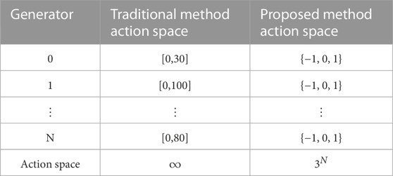
TABLE 1. Action space.

(5) Reward function. The reward function represents the reward value obtained by the agent after taking a certain action. The optimization goal is to obtain the maximum reward value. In view of the combination optimization problem of the grid section, this paper designs five types of rewards: 1) system cost rewards, 2) power flow limitation rewards, 3) load balancing rewards, 4) clean energy consumption rewards, and 5) generator unit limitation rewards. The purpose of optimizing the reward function is to minimize the system cost and maximize the proportion of clean energy on the premise that the power flow does not exceed the boundary, the output of the generator unit does not exceed the boundary, and the load is balanced in the grid system.

For each time step t, the evaluation score R_t of the system is calculated as follows:

$R_t=\sum _{i=1}^5{r}_{i,t},(6)$

where r_i,t is the reward of the ith type at the time step t. For simplicity, the subscript in the following formulas is omitted. Specifically, the calculation of each type of reward is as follows:

1) System cost (positive reward) with the value range of A₀*[0,100]:

$r_0=A_0*100*\min \left(\frac{C_{\min }}{{\sum }_{i=1}^N{C}_i},1\right),(7)$

where A₀ = 1 is the score weight. c_i is the cost of the corresponding generator, and the system has N generators in total. C_min is the normalization constant, which is the minimum cost of the system at a moment over a period of time. The lower the system cost is, the higher the reward score is.

2) Power flow limit reward (positive reward) with the value range of A₁*[0, 100]:

$r_1=A_1*\max \left(\left(100-\sum _{s=1}^S{r}^s\right),0\right),(8)$

where A₁ = 4 is the score weight, S is the total number of sections, and r^s is the reward value of the sth section. It is calculated according to different situations (over-limit or normal). In over-limit situations (that is, exceeding the upper or lower limit of the predetermined value), severe penalties are imposed, whereas under normal circumstances, there is no penalty. The specific calculation method is as follows:

$r^s=\left\{\begin{array}{c}\frac{\left|P_s-P_s^{\min }\right|}{10},P_s<P_s^{\min },\hfill \\ 0,P_s^{\min }<=P_s<=P_s^{\max },\hfill \\ \frac{\left|P_s-P_s^{\max }\right|}{10},P_s>P_s^{\max }\hfill \end{array}\right.(9)$

where P_s is the power flow of section s, $P_s^{\mathit{max}}$ is the upper limit of section s, and $P_s^{\mathit{min}}$ is the lower limit of section s. The denominator number in the equation is a parameter that restricts the severity of punishment, and 10 is a suitable figure for restricting the power flow.

3) Load balance reward (positive reward) with the value range of A₂*[0, 100]:

$r_2=A_2*\max \left(100*\left(1-\frac{\left|\mathrm{L}-{\sum }_{i=1}^N{P}_i\right|}{\left(0.1*L\right)}\right),0\right),(10)$

where A₂ = 3 is the score weight, L represents the total real load of the system at time t, and the denominator 0.1*L is a normalization parameter that is set according to the comprehensive consideration of ultra-short-term forecast deviation and score interval. P_i is the active power output of generator unit i, and N is the total number of generator units.

4) Clean energy consumption reward (positive reward) with the value range of A₃*[0, 100]:

$r_3=A_3*100*\frac{1}{M}\sum _{i=1}^M\mathit{min}\left(1,\frac{P_i}{P_i^{\mathit{max}}}\right),(11)$

where A₃ is the score weight, P_i represents the active power output of the clean energy generator unit i, and $P_i^{\mathit{max}}$ represents the maximum output of the clean energy generator unit i. In order to avoid the denominator being 0 when calculating the score, when $P_i^{\mathit{max}}$ is zero, the reward of generator unit i will be zero. There are a total of M clean energy generators.

5) Generator unit limit reward (positive reward) with the value range of A₄*[0, 100]:

$r_4=A_4*\mathit{max}\left(\left(100-\sum _{i=1}^N{r}^i\right),0\right),(12)$

where A₄ = 1 is the score weight, N is the total number of units, and rⁱ is the reward value of the sth generator. It is calculated according to different situations (over-limit or normal). In over-limit situations (that is, exceeding the upper or lower limit of the predetermined value), severe penalties are imposed, whereas under normal circumstances, there is no penalty. The specific calculation method is as follows:

$r^i=\left\{\begin{array}{c}\frac{\left|P_i-P_i^{\min }\right|}{10},P_i<P_i^{\min },\hfill \\ 0,P_i^{\min }<=P_i<=P_i^{\max },\hfill \\ \hfill \frac{\left|P_i-P_i^{\max }\right|}{10},P_i>P_i^{\max }\hfill \end{array}\right.(13)$

where P_i is the active output of generator i, $P_i^{\mathit{max}}$ is the upper limit of the active output of generator unit i, and $P_i^{\mathit{min}}$ is the lower limit of the active output of generator i.

3.3 Constrained reinforcement learning loss

In the AC algorithm, the critic is trained to fit the reward. Its loss function is as follows:

$L_{critic}=\frac{1}{N}\sum _i^N\left(G_t-V\left(s_{t}0\right)\right),(14)$

where G_t is R_t+1 + γR_t+2 + ⋯ + γⁿ⁻¹R_t+n + γⁿQ (s_t+n), and the actor is trained to find the optimal action a for the following minimization problem:

$\begin{array}{ll}\hfill \text{\hspace{0.17em}minimize\hspace{0.17em}}{L}_{\text{actor\hspace{0.17em}}}& =w_1\left|\mathrm{L}-\sum _{i\in I}{a}_i\right|+w_2\sum _{s\in S}\left|P_s\left(a\right)-P_s^{\max }\right|\hfill \\ \hfill & -w_3\sum _{i\in I_{ne}}\frac{a_i}{a_i^{\max }}+w_4\sum _{i\in I}{c}_i{a}_i,\hfill \end{array}(15)$

where w₁, w₂, w₃, and w₄ are the weight values of each item, L represents the total load of the grid system, a_i represents the active power output of the ith generator, I represents the set of all generators, S represents the set of all grid sections, P_s(a) represents the power flow value of the section s, and a is the output of the generator unit. $P_s^{\mathit{max}}$ is the maximum power flow of the section s, I_ne represents the clean energy generator set, $a_i^{\mathit{max}}$ represents the maximum active output of the ith clean energy generator, and c_i represents the cost coefficient of the ith generator.

However, in the aforementioned formula, the two strong constraints, namely, load balance and power flow constraints, are regarded as objective functions with weights, which lead to the inability of the algorithm to obtain a stable solution in principle. Therefore, this paper proposes a constrained reinforcement learning loss (CRLL) algorithm as follows:

$minimize{L}_{actor\underline{}constrained}=-W_1\sum _{i\in I}\frac{a_i}{a_i^{\mathit{max}}}+w_2\sum _{i\in I}{c}_i{a}_i,(16)$

$\text{\hspace{0.17em}s.t.\hspace{0.17em}}\left\{\begin{array}{c}\mathrm{L}-{\sum }_{i\in I}{a}_i=0\hfill \\ P_s\left(a\right)<=P_s^{\max }.\hfill \end{array}\right.$

While satisfying the load balance and power flow constraints, the aforementioned objective functions can fit those actions that maximize clean energy consumption and minimize cost. It restores the essence of the grid section combination optimization problem, which is more conducive to the convergence of the reinforcement learning algorithm. This paper incorporates this loss into the training of the reinforcement learning algorithm by using Lagrangian constraints.

3.4 Training method and process

This paper chooses the actor–critic reinforcement learning algorithm. The implementation of DRL combined with CRLL is shown in Algorithm 1. The training process is as follows:

1) First, generate the sample data using the PYPOWER simulator. Then, clear the cache in the experience pool, set the initial state of the power system, and reset the reward value.

2) Input the observed state s_t of the current grid section system into the policy network, and obtain the active power output a_t of the generator unit through the policy network.

3) Input the output a_t of the generator unit into the reinforcement learning environment, and obtain the grid state s_t+1 in the following stage, the reward value r corresponding to the current policy, and the completion state done.

4) Save the grid state s_t, the next moment’s state s_t+1, the output policy a_t, the current reward value r, and the completion state done into the experience pool.

5) Judge whether the current experience pool has reached the upper limit of capacity. If the experience pool has not reached the limit, repeat Step 3; otherwise, go to Step 6.

6) When the accumulated data in the experience pool reach the batch size, they will be input into the policy network and value network as training data to train the network parameters. Then, return to Step 1.

3.5 Annealing optimization algorithm

In the DRL method described previously, the action space is discretized, so the granularity of the action output by the model is not fine enough, resulting in the obtained solution being far beyond the optimal solution. In view of this problem, the annealing algorithm (Bakirtzis et al., 2002) is used after the proposed DRL algorithm to optimize the output of the generator unit. In this paper, we called it an annealing optimization algorithm. It can further improve the proposed DRL method to find the optimal fine-grained solution.

The annealing algorithm is a global optimization method based on a simulated physical annealing process. The basic idea of the algorithm is to start from an initial solution, continuously perturb the current solution randomly, and choose to accept the new solution or keep the current solution according to a certain probability. The function that accepts a new solution with a certain probability is called the “acceptance criterion.” The acceptance criterion allows the algorithm to perform a random walk in the search space and gradually reduces the temperature (that is, reduces the probability of accepting a new solution) until it reaches a stable state.

In the annealing optimization algorithm, the temperature parameter is usually used to control the variation in the acceptance criterion. At the beginning of the algorithm, the temperature is relatively high, so it tends to accept the new solutions according to the acceptance criterion. Therefore, a large-scale random search can be performed in the search space. As time goes by, the temperature gradually decreases, and it becomes much more difficult to accept the new solution, making the search process gradually stabilized. Eventually, the algorithm arrives at a near-optimal solution.

The annealing optimization algorithm is often used to solve nonlinear optimization problems, especially those with a large number of local optima. The advantage of the algorithm is that it can avoid falling into a local optimal solution and can perform a global search in the search space. In this paper, the annealing optimization algorithm is initialized by the output of the DRL model. The process of the annealing algorithm is as follows:

(1) Initialize the temperature T and the initial solution x.

(2) At the current temperature, produce a new solution x′ by using a random perturbation to the current solution.

(3) Calculate the energy difference ΔE between the new solution and the current solution.

(4) If ΔE < 0, accept the new solution as the current solution.

(5) If ΔE ≥ 0, accept the new solution as the current solution with a probability P = exp (−ΔE/T).

(6) Lower the temperature T.

(7) Repeat Steps 2–6 until the temperature drops to the end temperature or the maximum number of iterations is reached.

The algorithm flow chart is described in Figure 2.

FIGURE 2

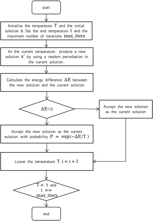
FIGURE 2. Flow chart of the annealing optimization algorithm.

4 Case study

To verify the effectiveness of the proposed method, this paper uses an IEEE 118-bus system. It consists of 118 buses, 54 generators, and 186 branches, representing a real power system network. The generators Gen 1 ∼Gen 20 are set as the new energy units in this paper.

The computing environment is based on PYPOWER. The scheduling cycle is set to 15 min a day. According to the aforementioned description of MDP, the AC algorithm has 20 dimensions of state space. The dimension of the action space is set to 54. The detailed setting of hyper-parameters is shown in Table 2. The experiment runs on the Apple M1 Pro silicon with 8-core CPU and 16 GB memory. Figure 3 shows that the proposed model converges after approximately 900 episodes. As for the training time, the models converge after approximately 1 hour.

TABLE 2

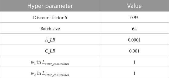
TABLE 2. Setting of hyper-parameters.

FIGURE 3

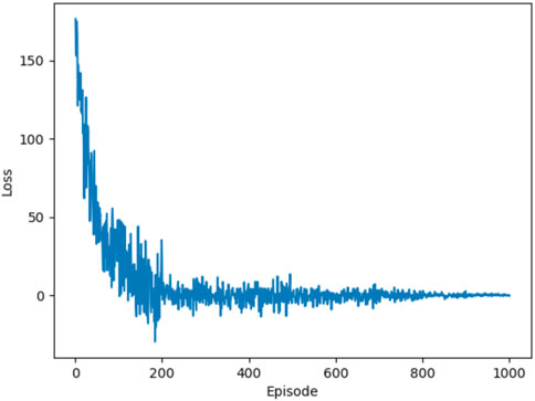
FIGURE 3. Proposed model convergence after approximately 900 episodes.

Using the environment and the AC algorithm based on the CRLL in this paper, the agent maximizes the reward by adjusting the active power generated by the generator unit while minimizing the total cost and enhancing the new energy consumption. It can be seen from Figure 4 that the AC algorithm based on CRLL can converge and obtain the solution after 30 episodes. In contrast, it can be found that the traditional AC algorithm (vanilla AC) cannot achieve convergence within the same episode, and it cannot always reach the optimal solution. Table 3 shows that vanilla AC training takes much longer than 4 h, but after using the proposed CRLL, the model convergence time is reduced to 1 h. By comparison, it can be seen that the proposed loss function plays a vital role in the stability of the solution and the convergence speed of model training.

FIGURE 4

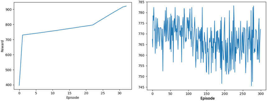
FIGURE 4. Scheduling results of the AC algorithm based on CRLL and the traditional AC algorithm.

TABLE 3

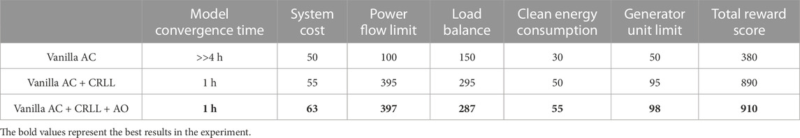
TABLE 3. Control experiment to verify the effectiveness of the proposed method. CRLL, constrained reinforcement learning loss; AO, annealing optimization algorithm.

In Table 3, the experiment compares the results of three methods: 1) vanilla AC, 2) vanilla AC plus CRLL, and 3) vanilla AC plus CRLL and the annealing optimization algorithm. The scoring for all three methods is made up of five items. The full scores of system cost, power flow limit, load balance, clean energy consumption, and generator unit limit are 100, 400, 300, 100, and 100, respectively. Among them, power flow limit, load balance, and generator unit limit are strong constraints in the power grid section system. The goal of the proposed method is to make these three items close to full scores.

As shown in Table 3, the scores of all indicators have been greatly improved due to the proposed loss function, meeting the safety requirements of the power grid. The total reward score of the vanilla AC is 380, while the AC algorithm with CRLL achieves a higher total reward score of 890.

In addition, combining DRL with the annealing optimization algorithm further improved the accuracy of the solution. In Table 3, the average reward score of the final model is 910, among which the power flow limit, generator unit limit, and load balance rewards all reached almost full scores. It indicates that the addition of the annealing optimization algorithm further improves the performance of the algorithm and obtains a fine-grained optimal solution.

The results of the three methods are also shown in Figure 5 as a histogram. It intuitively demonstrates that the algorithm proposed in this paper is able to optimize the objective function under multiple strong constraints. So, it can be concluded that the method proposed in this paper is effective and can meet the requirements of online optimization and real-time control of the grid section.

FIGURE 5

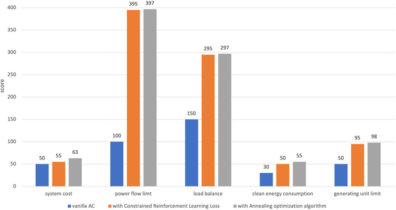
FIGURE 5. Control experiment to verify the effectiveness of the proposed method.

5 Conclusion

In the face of the high proportion of new energy generator units and complex constrained environments, this paper uses the deep reinforcement learning algorithm of simplified action space, together with CRLL, to search for the optimal active power output of generators. It also uses the annealing optimization algorithm to avoid the local optimal solution. The formulation and implementation process are introduced in detail. The test results on the IEEE 118-bus system show that the proposed method has good performance and is suitable for scheduling problems. In this paper, system cost and clean energy consumption have not reached full scores yet, and future improvement work can be committed to achieve better results. Another attempt is to use a multi-checkpoint and multi-process model inference approach that can both speed up the inference and improve the indicators by allowing each checkpoint to focus on different metrics.

Algorithm 1.: AC training based on CRLL

Require: episode ep, discount factor γ, LR_a, LR_c, batch size b, θ_a, θ_c, maxsize

 1:  while i < ep do

 2:   reward = 0; reset env; reset the experience pool

 3:   collect the trajectory information including (S_t, A_t, R_t, S_t+1)

 4:   if poolsize < maxsize then

 5:    pool ← (S_t, A_t, R_t, S_t+1)

 6:   end if

 7:   if poolsize > b then

 8:    update θ_a with L_{actor_constrained}

 9:    update θ_c with L_critic

 10:   end if

 11:  end while

Data availability statement

Publicly available datasets were analyzed in this study. These data can be found at: http://labs.ece.uw.edu/pstca/pf118/pg_tca118bus.htm.

Author contributions

HZ: methodology, writing–original draft, and conceptualization. ZW: conceptualization, software, and writing–original draft. YH: writing–original draft and investigation. QF: writing–original draft and data curation. SL: writing–original draft and methodology. GM: validation, writing–original draft, and software. WL: formal analysis, visualization, and writing–review and editing. QY: conceptualization, funding acquisition, resources, supervision, and writing–review and editing.

Funding

The author(s) declare that no financial support was received for the research, authorship, and/or publication of this article.

Conflict of interest

The authors declare that the research was conducted in the absence of any commercial or financial relationships that could be construed as a potential conflict of interest.

Publisher’s note

All claims expressed in this article are solely those of the authors and do not necessarily represent those of their affiliated organizations, or those of the publisher, the editors, and the reviewers. Any product that may be evaluated in this article, or claim that may be made by its manufacturer, is not guaranteed or endorsed by the publisher.

References

Alshammari, M. E., Ramli, M. A., and Mehedi, I. M. (2022). Hybrid chaotic maps-based artificial bee colony for solving wind energy-integrated power dispatch problem. Energies 15, 4578. doi:10.3390/en15134578

CrossRef Full Text | Google Scholar

Ardakani, A. J., and Bouffard, F. (2018). “Prediction of umbrella constraints,” in Proceedings of the 2018 Power Systems Computation Conference (PSCC), Dublin, Ireland, June 2018 (IEEE), 1–7.

Google Scholar

Aydın, D., and Özyön, S. (2013). Solution to non-convex economic dispatch problem with valve point effects by incremental artificial bee colony with local search. Appl. Soft Comput. 13, 2456–2466. doi:10.1016/j.asoc.2012.12.002

CrossRef Full Text | Google Scholar

Bakirtzis, A. G., Biskas, P. N., Zoumas, C. E., and Petridis, V. (2002). Optimal power flow by enhanced genetic algorithm. IEEE Trans. power Syst. 17, 229–236. doi:10.1109/tpwrs.2002.1007886

CrossRef Full Text | Google Scholar

Diehl, F. (2019). “Warm-starting ac optimal power flow with graph neural networks,” in Proceedings of the 33rd Conference on Neural Information Processing Systems (NeurIPS 2019), Munich, Germany, 1–6.

Google Scholar

Gherbi, F., and Lakdja, F. (2011). “Environmentally constrained economic dispatch via quadratic programming,” in Proceedings of the 2011 International Conference on Communications, Computing and Control Applications (CCCA), Hammamet, Tunisia, March 2011 (IEEE), 1–5.

CrossRef Full Text | Google Scholar

Guo, L., Guo, J., Zhang, Y., Guo, W., Xue, Y., and Wang, L. (2022). “Real-time decision making for power system via imitation learning and reinforcement learning,” in Proceedings of the 2022 IEEE/IAS Industrial and Commercial Power System Asia (I&CPS Asia), Shanghai, China, July 2022 (IEEE), 744–748.

CrossRef Full Text | Google Scholar

Irisarri, G., Kimball, L., Clements, K., Bagchi, A., and Davis, P. (1998). Economic dispatch with network and ramping constraints via interior point methods. IEEE Trans. Power Syst. 13, 236–242. doi:10.1109/59.651641

CrossRef Full Text | Google Scholar

Jiang, L., Wang, J., Li, P., Dai, X., Cai, K., and Ren, J. (2021). “Intelligent optimization of reactive voltage for power grid with new energy based on deep reinforcement learning,” in Proceedings of the 2021 IEEE 5th Conference on Energy Internet and Energy System Integration (EI2), Taiyuan, China, October 2021 (IEEE), 2883–2889.

CrossRef Full Text | Google Scholar

Larouci, B., Ayad, A. N. E. I., Alharbi, H., Alharbi, T. E., Boudjella, H., Tayeb, A. S., et al. (2022). Investigation on new metaheuristic algorithms for solving dynamic combined economic environmental dispatch problems. Sustainability 14, 5554. doi:10.3390/su14095554

CrossRef Full Text | Google Scholar

Lillicrap, T. P., Hunt, J. J., Pritzel, A., Heess, N., Erez, T., Tassa, Y., et al. (2015). Continuous control with deep reinforcement learning. Available at: https://arxiv.org/abs/1509.02971.

Google Scholar

Liu, X., Liu, J., Zhao, Y., and Liu, J. (2022). “A deep reinforcement learning framework for automatic operation control of power system considering extreme weather events,” in Proceedings of the 2022 IEEE Power & Energy Society General Meeting (PESGM), Denver, CO, USA, July 2022 (IEEE), 1–5.

CrossRef Full Text | Google Scholar

Mnih, V., Kavukcuoglu, K., Silver, D., Graves, A., Antonoglou, I., Wierstra, D., et al. (2013). Playing atari with deep reinforcement learning. Available at: https://arxiv.org/abs/1312.5602.

Google Scholar

Modiri-Delshad, M., Kaboli, S. H. A., Taslimi-Renani, E., and Abd Rahim, N. (2016). Backtracking search algorithm for solving economic dispatch problems with valve-point effects and multiple fuel options. Energy 116, 637–649. doi:10.1016/j.energy.2016.09.140

CrossRef Full Text | Google Scholar

Sayed, A. R., Wang, C., Anis, H., and Bi, T. (2022). Feasibility constrained online calculation for real-time optimal power flow: A convex constrained deep reinforcement learning approach. IEEE Trans. Power Syst., 1–13. doi:10.1109/tpwrs.2022.3220799

CrossRef Full Text | Google Scholar

Shchetinin, D., De Rubira, T. T., and Hug, G. (2018). On the construction of linear approximations of line flow constraints for ac optimal power flow. IEEE Trans. Power Syst. 34, 1182–1192. doi:10.1109/tpwrs.2018.2874173

CrossRef Full Text | Google Scholar

Silver, D., Lever, G., Heess, N., Degris, T., Wierstra, D., and Riedmiller, M. (2014). “Deterministic policy gradient algorithms,” in Proceedings of the International conference on machine learning (Pmlr), Beijing, China, June 2014, 387–395.

Google Scholar

Sutton, R. S. (1988). Learning to predict by the methods of temporal differences. Mach. Learn. 3, 9–44. doi:10.1007/bf00115009

CrossRef Full Text | Google Scholar

Sutton, R. S., McAllester, D., Singh, S., and Mansour, Y. (1999). Policy gradient methods for reinforcement learning with function approximation. Adv. neural Inf. Process. Syst. 12.

Google Scholar

Yan, Z., and Xu, Y. (2020). Real-time optimal power flow: A Lagrangian based deep reinforcement learning approach. IEEE Trans. Power Syst. 35, 3270–3273. doi:10.1109/tpwrs.2020.2987292

CrossRef Full Text | Google Scholar

Yin, L., Yu, T., Zhang, X., and Yang, B. (2018). Relaxed deep learning for real-time economic generation dispatch and control with unified time scale. Energy 149, 11–23. doi:10.1016/j.energy.2018.01.165

CrossRef Full Text | Google Scholar

Zhan, J., Wu, Q., Guo, C., and Zhou, X. (2013). Fast λ-iteration method for economic dispatch with prohibited operating zones. IEEE Trans. power Syst. 29, 990–991. doi:10.1109/tpwrs.2013.2287995

CrossRef Full Text | Google Scholar

Zhao, Y., Liu, J., Liu, X., Yuan, K., Ren, K., and Yang, M. (2022). “A graph-based deep reinforcement learning framework for autonomous power dispatch on power systems with changing topologies,” in Proceedings of the 2022 IEEE Sustainable Power and Energy Conference (iSPEC), Perth, Australia, December 2022 (IEEE), 1–5.

CrossRef Full Text | Google Scholar

Zhou, Y., Lee, W.-J., Diao, R., and Shi, D. (2021). Deep reinforcement learning based real-time ac optimal power flow considering uncertainties. J. Mod. Power Syst. Clean Energy 10, 1098–1109. doi:10.35833/mpce.2020.000885

CrossRef Full Text | Google Scholar

Zivic Djurovic, M., Milacic, A., and Krsulja, M. (2012). “A simplified model of quadratic cost function for thermal generators,” in Proceedings of the 23rd International DAAAM Symposium, Zadar, Croatia, October 2012, 24–27.

CrossRef Full Text | Google Scholar