Short-term wind power prediction based on anomalous data cleaning and optimized LSTM network

Wind power prediction values are often unstable. The purpose of this study is to provide theoretical support for large-scale grid integration of power systems by analyzing units from three different regions in China and using neural networks to improve power prediction accuracy. The variables that have the greatest impact on power are screened out using the Pearson correlation coefficient. Optimize LSTM with Lion Swarm Algorithm (LSO) and add GCT attention module for optimization. Short-term predictions of actual power are made for Gansu (Northwest China), Hebei (Central Plains), and Zhejiang (Coastal China). The results show that the mean absolute percentage error (MAPE) of the nine units ranges from 9.156% to 16.38% and the root mean square error (RMSE) ranges from 1.028 to 1.546 MW for power prediction for the next 12 h. The MAPE of the units ranges from 11.36% to 18.58% and the RMSE ranges from 2.065 to 2.538 MW for the next 24 h. Furthermore, the LSTM is optimized by adding the GCT attention module to optimize the LSTM. 2.538 MW. In addition, compared with the model before data cleaning, the 12 h prediction error MAPE and RMSE are improved by an average of 34.82% and 38.10%, respectively; and the 24 h prediction error values are improved by an average of 26.32% and 20.69%, which proves the necessity of data cleaning and the generalizability of the model. The subsequent research content was also identified.

1 Introduction

In the context of global promotion of low-carbon economy and energy revolution, reducing fossil energy combustion, accelerating the development and utilization of renewable energy has become the general consensus and unanimous action of the international community; wind energy, as one of the most commercialized renewable energy sources, has achieved large-scale development and application worldwide, and wind power has become an essential component of new electricity systems González-Sopeña et al. (2021); Diaconita et al. (2022). Wind power has more than 700 GW of installed capacity worldwide as of 2023, and it is still expanding quickly every year. China, the United States, Germany, India, Spain, and the United Kingdom are among those that produce the most wind energy globally Li (2022); Ding et al. (2022). However, due to the high volatility of wind power caused by environmental factors, the prediction becomes inaccurate and can directly affect the safety of grid connection. As a result, one of the hottest areas of research right now is how to efficiently increase prediction accuracy Chen and Lin (2022); Ramasamy et al. (2015); Chandel et al. (2014b); Chandel et al. (2014a).

At present, due to the limitation of technical means, the power prediction by neural network is generally a short-term prediction. In this case, a lot of data from the SCADA system, but the system records and stores the operation data in the inevitable existence of noise and faults and other anomalous data, according to the distribution of the data in the power curve of the unit, the anomalous data is divided into: the bottom of the pile-up type, deviation from the power band type, the middle of the pile-up type, the type of discrete several categories Zhao et al. (2022); Uddin and Sadiq (2022). These data cannot truly reflect the operating state of the unit, and only the data after removing the abnormal data can reflect the unit’s will-con state, and can be used to train the prediction model of the unit Wang et al. (2022a). For this reason, scholars began to look for methods that can effectively remove the abnormal data. Literature 12 uses the K-means clustering algorithm to remove the abnormal power data SheenaKurian and Mathew (2023), but the deletion rate of this algorithm is high, which destroys the temporal sequence of the original wind sequence and affects the later prediction results; Literature 13 utilizes the quartile method to clean the data Schubert et al. (2017), which is generalizable but ineffective in identifying the high percentage of abnormal data; literature 14 combines the combination of the quartile method and DBSCAN in Literature 11 enhances the identification of anomalous data Wang et al. (2022b), but it is more sensitive to the parameter settings and decreases the efficiency of prediction.

In addition, meteorological conditions are also a factor that affects the accuracy of prediction. Scholars have considered various methods to find out the factors affecting the output power results in order to make the study effective for practical use. For example, Jordan Nielson et al. used feed-forward back-propagation (FFBP) ANN model to predict the power output of individual wind turbines from the turbine itself, and improved the accuracy of power generation prediction by studying the atmospheric input variables in order to construct a power curve Meka et al. (2021); Rajitha Meka et al. used Pearson’s algorithm to discuss the factors that include ground temperature, wind speed, atmospheric pressure, wind direction, and more than ten types of meteorological data that have the potential to affect the power transmission results, and the most relevant variables to the output power were used as inputs to the temporal convolutional network (TCN), and the validity of the methodology was confirmed by a multistep prediction Nielson et al. (2020). In addition, Principal Component Analysis (PCA) and shape value method were also used as correlation analysis, and the results obtained from all of the above methods showed that wind speed is the most important factor affecting the output power.

In terms of model selection, the literature Liu et al. (2018) uses support vector machine (SVM) for regression analysis, but due to the choice of kernel parameters, its generalization ability is weak and its learning capacity is insufficient for large-scale wind farm data, resulting in fluctuations in prediction results. The literature Krishna et al. (2021) also uses extreme learning machine (ELM) to simplify the network, which increases prediction accuracy to a certain extent, but because the hidden layer analytic complexity is low, it is difficult to generalize the results. Other researchers attempt to use the classical BP Li et al. (2022) network and LSTM Malakouti et al. (2022) network, both of which have achieved good prediction results, but the application to the actual wind power also has issues similar to those of SVM and ELM because the hidden layer and bias parameters in the network structure are random. As a result, the generalization ability decreases.

Researchers have begun to think about using some intelligent optimization algorithms to replace human optimization search because many underlying models call for the selection of debugging parameters, which significantly affects the efficiency of learning. For instance, the literature Hui et al. (2018) used the rich-poor optimization algorithm to optimize the parameters of the outlier robust learning machine to improve the generalization ability of the model, as well as the Optimize lstm based on improved whale algorithm Yang et al. (2022) and the variational modal decomposition and sparrow algorithm Wu and Wang (2021). Literature Wang et al. (2020) error correction is performed using RBF-based optimization LSSVM to increase the precision of the prediction outputs. These combined models, which were previously mentioned, have decreased prediction efficiency as a result of the addition of optimization algorithms, but have only slightly increased prediction accuracy. They are somewhat concerned with one thing but not the other, and the majority of them are only studied for one unit of a single wind farm without the support of more real data, which makes them weak arguments.

In order to solve the aforementioned problems, a KD-LSO-G-LSTM wind power short-term prediction model is developed in this study. The following are some of the research contributions.

1) For the anomalous data in the original power, first use the elbow method to decide on the optimal number of clusters, which not only can avoid the issue of manual selection leading to lower efficiency, but also can make the best detection effect. Then, use the K-means algorithm to clean the first class of anomalous data values, and DBSCAN to reject the second class of anomalous data. The effectiveness of the approach for cleaning wind power is tested in the paper using comparison and ablation experiments, respectively;

2) Proposed using the original LSTM neural network and adding the Gated Channel Transformation (GCT) attention mechanism module to enhance the network’s performance in the prior and subsequent moments;

3) Reducing the amount of time needed to discover the best settings for the G-LSTM by using the Lion Swarm method;

4) Nine wind turbines from three different regions of China (the Northwest, Central Plains, and Coastal) were chosen for simulation trials based on actual wind farm data in order to prevent model overfitting, and encouraging forecast results were produced.

2 Materials and methods

2.1 Abnormal data cleaning

2.1.1 K-means

The most fundamental and widely used clustering algorithm is K-means clustering. Contrary to classification and sequence labeling tasks, clustering is an unsupervised algorithm that divides samples into multiple categories based on the inherent relationship between data without knowing any sample labels in advance, producing high similarity between samples of the same category and low similarity between samples of different categories. The main concept behind it is to iteratively identify a division scheme of K clusters so that the loss function associated with the clustering result is minimized. Where the loss function is the sum of the squared deviations of each sample from the cluster centroid to which it belongs Jin and Han (2021).

$J\left(c,\mu \right)={\displaystyle \sum _{i=1}^M}{‖x_i-{\mu }_{ci}‖}^2(1)$

Where x_i represents the ith sample, and c_i is the cluster it belongs to, and μ_ci denotes the central point corresponding to the cluster, and M is the total number of samples. The core objective of K-means is to divide the given data set into K clusters and give the center corresponding to each sample data. These are the precise steps.

1) Data preprocessing, primarily data normalization;

2) Randomly select K center points, labeled as ${\mu }_k^0$;

3) Define the loss function:J(c, μ);

4) Equations 2, 3 should be repeated until J converges, where t denotes the number of iteration steps.

First, for each sample x_i, assign it to the nearest center:

$c_i^t<{-\mathit{argmin}}_k{‖x_i-{\mu }_k^t‖}^2(2)$

The center of each class is then recalculated for each class center k:

${\mu }_k^{t+1}<{-\mathit{argmin}}_k{\displaystyle \sum _{i:c_i^t}^b}{‖x_i-\mu ‖}^2(3)$

The main goal of K-means is to decrease J by fixing the center and changing the category that each sample belongs to. The two processes switch off, J drops monotonically until it reaches its minimal value, and at the same time, the centroid and the category into which the samples are divided.

2.1.2 DBSCAN abnormal data cleaning

One of the more exemplary density-based clustering algorithms is DBSCAN. It is able to combine clusters with adequate high density of areas into clusters and can be utilized in noisy spatial databases of variable forms in the clusters, in contrast to division and hierarchical clustering methods that define clusters as the greatest set of densely connected points Hahsler et al. (2019).

The core metrics of the algorithm are the neighborhood range radius and the minimum number of neighborhood points threshold, i.e., epsilon and minpts. The EPS neighborhood is defined as a circle with a center p and a radius epsilon. The number of data points in this neighborhood is m, which reflects the density of the cluster. minpts: The minimum number of data points, which is usually given directly. Based on the relationship between m and minpts, the data points can be distinguished as core points, boundary points, and outlier points. After dividing the data points, the algorithm divides the density relationship between two arbitrary data points in the same cluster into three categories: direct density reachable, density reachable, and density connected. Direct density reachable: if a point q is within the EPS neighborhood of data point p and data point q is the core point, then the center point p is directly density reachable from data point q. Density reachable: if data points p₁, p₂, … , p_n in a certain EPS neighborhood, if p_i of these data points can be directly density reachable p_i+1, then it is said that p₁ density up to p_n. Density connectivity: If a data point s is accessible by data point q and data point q, then data point q and data point q are said to be density connected.

2.2 Lion group algorithm

A suggested algorithm called LSO, which has a high optimization efficiency, is based on how lion prides hunt. The lion pride method divides the lions into three groups in order to solve the global optimization issue given the objective function: The lioness, the lioness, and the cub. Its parameters are defined as follows Lee et al. (2020).

1) For adult lions, the proportion factor β is a random number between 0 and 1, and the value of β is typically set at 0.5 to speed up convergence.

2) Lioness moving range perturbation factor α_f, the perturbation factor is defined as follows, and its purpose is to dynamically update the search range to promote convergence.

${\alpha }_f=step•\mathit{exp}{\left(-\frac{30}{T}\right)}^{10}(4)$

where: $step=0.1(\bar{H}-\bar{L})$ denotes the maximum step range of lion activity; t and T denote the current number of iterations as well as the maximum number of iterations, respectively; and denote the maximum and minimum mean values in the range of lion movement.

3) The range’s elongation or compression is controlled by the perturbation factor for cubs α_c, which is specified as follows:

${\alpha }_c=step•\left(\frac{T-t}{T}\right)(5)$

Suppose there are N lions in a D-dimensional algorithmic space, and let nLeader denote the number of adult lions, then:

$2\le nLeader\le \frac{N}{2}(6)$

There is one male lion in the pride and the remainder are females. The coordinate information of the ith (1 ≤ i ≤ N) lion is x_i = x_i1, x_i2, … , x_iD (1 ≤ i ≤ N). The number of adult lions is: nLeader = N*β, and the number of juvenile lions N − nLeader. Each of the three fulfills his responsibility while the male lion hunts for superiority, moves in a restricted region close to the ideal position. The position update formula is:

$x_i^{k+1}=g^k\left(1+\delta ‖p_i^k-g^k‖\right)(7)$

And the lioness needs to work with the other end to update, according to Equation 8:

$x_i^{k+1}=\frac{p_i^k+p_c^k}{2}\left(1+{\alpha }_f\tau \right)(8)$

Lion cubs are divided into three situations: hunting with the lioness, feeding with the lion king, and elite reverse learning. The process is shown below:

$x_i^{k+1}=\left\{\begin{array}{c}\frac{p_i^k+g^k}{2}\left(1+{\alpha }_c\tau \right),q\le \frac{1}{3}\hfill \\ \hfill \frac{p_m^k+p_i^k}{2}\left(1+{\alpha }_c\tau \right),\frac{1}{3}\le q\le \frac{2}{3}\hfill \\ \hfill \frac{p_i^k+g^{\prime k}}{2}\left(1+{\alpha }_c\tau \right),\frac{2}{3}\le q\le 1\hfill \end{array}\right.(9)$

$p_c^k$ is the historical optimal position of a randomly chosen hunting collaborative partner in the kth generation of the lioness pride, where is a pseudo-random number generated using the normal distribution N (0,1). $p_i^k$ represents the historical optimal solution for the kth generation of the ith lion, g^k represents the kth generation optimal position of the group. And: $g^{\prime k}=\bar{L}-\bar{H}-g^k$ is the position of the ith lion cub driven.$p_m^k$ represents the kth generation’s best placement for the cub to follow the lioness, and q is the probability factor, a random number produced using the uniform distribution U [0,1] Zhang et al. (2020).

2.3 LSTM

In many sequential tasks, long short-term memory (LSTM) is used, and it typically outperforms other sequential models like RNN when it comes to learning tasks involving vast amounts of data. The LSTM’s structure means that it can store more memories and that it can better manage which memories are kept and which ones are deleted at a particular time step. The LSTM’s structure means that it can better regulate which memories are kept and which ones are deleted at a certain time step. The cell structure is shown in Figure 1.

FIGURE 1

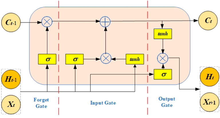
FIGURE 1. LSTM unit structure diagram.

According to the above figure, an LSTM cell consists of a memory cell C_t and three gate structures (input gate i_t, forgetting gate f_t, output gate o_t). At the moment t, the x_t represents the input data and h_t represents the hidden layer. ⊗ represents the vector outer product, ⊕ and represents the superposition operation Greff et al. (2015). The formula is as follows:

$f_t=\sigma \left(U_f{x}_t+W_f{h}_{t-1}+b_f\right)(10)$

$i_t=\sigma \left(U_i{x}_t+W_i{h}_{t-1}+b_i\right)(11)$

$u_t=\mathit{tanh}\left(U_u{x}_t+W_u{h}_{t-1}+b_u\right)(12)$

$c_t=f_t*c_{t-1}+i_t*u_t(13)$

$o_t=\sigma \left(U_o{x}_t+W_o{h}_{t-1}+b_o\right)(14)$

$h_t=o_t*\mathit{tanh}\left(c_t\right)(15)$

where U and W are the matrix weights, b is the offset, and σ is the Sigmoid function.

3 Model structure of this paper

Figure 2 depicts the model’s flow in this article. The plan is to separate the data gathered by the SCADA system into a training set and a test set, count the number of clusters using the Elbow method, remove and clean the data gathered in the low power region (the first category), and the high power region (the second category), using K-means and DBSCAN, respectively. After that, the two sets of data are combined to create a new wind power sequence, which is then input to LSO-G-LSTM to determine the prediction results. Below is a description of the LSO-G-LSTM algorithm flow and the G-LSTM network structure, respectively.

FIGURE 2

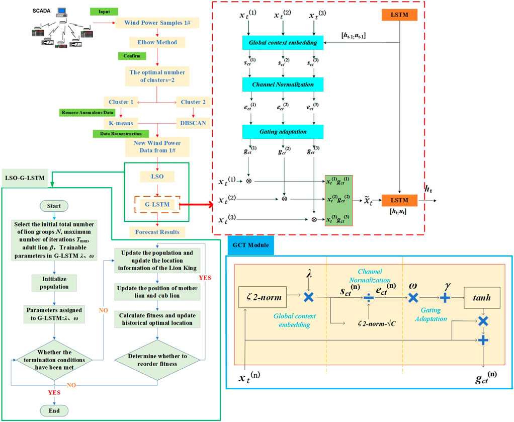
FIGURE 2. Flow chart of the model in this paper.

Even though LSTM can explain the inherent correlation of wind power output data, the wind power output varies significantly due to variations in wind speed and other factors, and predictions made using simply LSTM networks are frequently wrong. When building the model, the GCT attention mechanism module, which is compact and easy to understand, takes up little room, and the straightforward threshold settings make it easy to visualize the behavioral value of the GCT: competition OR synergy. To improve prediction accuracy, adding GCT to the LSTM coding layer can dynamically vary the contribution of various characteristics to the output and the weights of the input features Zhang et al. (2022). The red dashed box in the figure depicts the G-LSTM unit’s construction. The blue box in the illustration represents the GCT module. First assume that the input $x_t^{(n)}$ denotes the activation features in the CNN, and its time series is $X=[x_1,x_2,\dots ,x_t]={[x^{(1)},x^{(2)},\dots ,x^{(n)}]}^T$, the expanded matrix expression is:

$X=\left[\begin{array}{ccc}\hfill x_1^{\left(1\right)}\hfill & \hfill \cdots \hfill & \hfill x_1^{\left(n\right)}\hfill \\ \hfill ⋮\hfill & \hfill \ddots \hfill & \hfill ⋮\hfill \\ \hfill x_T^{\left(1\right)}\hfill & \hfill \cdots \hfill & \hfill x_T^{\left(n\right)}\hfill \end{array}\right]\in R^{T\times n}(16)$

Where $x_t=[x_t^{(1)},x_t^{(2)},\dots ,x_t^{(n)}](1\le t\le T)$ denotes a number of meteorological feature sets at moment t.

From the G-LSTM structure diagram, the relevant meteorological features are input to the attention mechanism at moment t. Combining the output of the hidden unit h_t−1 and the memory information μ_t−1 at moment t − 1, the GCT performs the following transformation on the input data sequence:

$g_{ct}^{\left(n\right)}=F\left(x_t^{\left(n\right)}\left|\lambda ,\omega ,\gamma \right.\right)(17)$

Where, λ, ω, γ are trainable parameters contribute to the adaptiveness of the embedded output, λ is used to control the activation threshold, ω, γ they determine the behavioral performance of the GCT in each channel. According to the figure shown, the GCT is divided into three components Lu et al. (2021).

The first part is Global Context Embedding, given the embedding parameters $\lambda =[{\lambda }_{1t}^{(1)},\dots ,{\lambda }_{ct}^{(n)}]$, defined as follows:

$s_{ct}^{\left(n\right)}={\lambda }_{ct}^{\left(n\right)}{‖x_t^{\left(n\right)}‖}^2={\lambda }_{ct}^{\left(n\right)}{\left\{\left[{\displaystyle \sum _{i=1}^H}{\displaystyle \sum _{j=1}^W}{\left(x_t^{\left(n\right)i,j}\right)}^2\right]+\epsilon \right\}}^{\frac{1}{2}}(18)$

where ɛ is used to avoid the reciprocal to 0. The trainable parameter ${\lambda }_{ct}^{(n)}$ are used to control the importance of different channels.

The second part is Channel Normalization, which, based on literature experience, uses ζ₂ for cross-channel feature normalization, which is defined at this point as follows:

$e_{ct}^{\left(n\right)}=\frac{\sqrt{C}{s}_{ct}^{\left(n\right)}}{{‖s‖}_2}=\frac{\sqrt{C}{s}_{ct}^{\left(n\right)}}{{\left[\left({\sum }_{c=1}^C{\left(s_{ct}^{\left(n\right)}\right)}^2+\epsilon \right)\right]}^{\frac{1}{2}}}(19)$

$\sqrt{C}$ is the scale factor to normalize $e_{ct}^{(n)}$, thus avoiding the scale being too small. The third part, Gating Adaptation, by introducing a gating mechanism, GCT can help to promote competitive OR synergistic relationships of neurons. The definition is as follows:

$g_{ct}^{\left(n\right)}=x_t^{\left(n\right)}\left[1+\mathit{tanh}\left({\gamma }_c{e}_{ct}^{\left(n\right)}+{\omega }_c\right)\right](20)$

The GCT obtains channel competition when the additional trainable parameters are positive; when they are negative, it receives a synergistic relationship. With this functionality, the network performs more robustly and the training data is more steady when making predictions.

The correlation characteristics considering the contribution of different meteorological elements ${\tilde{x}}_t$ are obtained by multiplying the characteristic correlation coefficients $g_{ct}^{(n)}$ with the corresponding meteorological characteristic values $x_t^{(n)}$:

${\stackrel{\sim }{x}}_t=\left[g_{ct}^{\left(1\right)}{x}_t^{\left(1\right)},g_{ct}^{\left(2\right)}{x}_t^{\left(2\right)},\dots ,g_{ct}^{\left(n\right)}{x}_t^{\left(n\right)}\right](21)$

Obviously, the relevant correlated weather feature matrix of the input can be extracted flexibly by the feature attention mechanism. The hidden layer state h_t is then updated according to the following equation:

$h_t=f_1\left(h_{t-1},{\stackrel{\sim }{x}}_t\right)(22)$

Through the feature attention mechanism, the input layer considers the correlation between the input meteorological features and the output power, strengthens the key factors affecting the wind power output, and adaptively extracts the contribution of each feature to improve prediction accuracy. f₁ is the LSTM network unit, and the input is no longer the original meteorological feature values but the weighted features considering the magnitude of correlation.

3.1 LSO-G-LSTM

Based on the above theory, a wind power prediction model named LSO-G-LSTM is built in this paper whose steps are as follows:

Step 1: The total number of initial lions N, the maximum number of iterations T_max, the adult lions β, and the trainable parameters λ, ω, γ of the G-LSTM neural network are selected.

Step 2: Generate the initial population $p_i^k=(c_i^k,g_i^k)$.

Step 3: Calculate the resulting fitness, assign it to the activation parameter λ and the threshold parameters ω, γ in the GCT, and update the information of the male lion’s position.

Step 4: Update the lioness and cub location information according to Eqs 8, 9.

Step 5: Judge whether the male, female and cubs should be sorted and renewed according to the degree of adaptation.

Step 6: Determine whether the optimal parameters are found, if yes, output; if no, repeat steps three to six until the optimal is found or the maximum number of iterations is reached.

4 Case study

In this paper, the wind power historical data of 2017–2018 from three power plants in Northwest, Central and Coastal China are selected respectively, in which three units are selected from each power plant and sampled at 10-min intervals, and 10,000 data are taken from each group. LSTM, LSO-LSTM, and KD-LSO-G-LSTM models are constructed respectively, which are used to predict the wind power in the next 12 and 24 h, and the prediction results are compared with similar models in other literatures to analyze the errors.

PyCharm is the experimental platform. The operating system is 64 for Windows 10, the programming language is Python version 3.8, and the running RAM is 16.0 GB.

First, the meteorological data and unit characteristics of the three wind farms collected through the SCADA system were correlated and analyzed, so as to select the variables suitable for use as model inputs. The Pearson correlation coefficient method was used to analyze the degree of contribution of wind speed (ws), wind direction (wd), air temperature (T), atmospheric pressure (Pa), wind turbine rotational speed (rs), and relative humidity (RH) data to power (wp). The quotient of the covariance and standard deviation between two variables is defined by the Pearson correlation coefficient between the two variables as shown in the following equation.

${\rho }_{x,y}=\frac{cov\left(x,y\right)}{{\delta }_x{\delta }_y}=\frac{E\left[\left(x-{\mu }_x,y-{\mu }_y\right)\right]}{{\delta }_x{\delta }_y}(23)$

Where, ρ_x,y denotes the overall correlation coefficient;covx,y denotes the covariance; E denotes the mathematical expectation;δ_x, δ_y represents the product of the standard deviation; and x-μ_x and y-μ_y denotes the value of its mean difference, respectively. The sample Pearson correlation coefficient is shown in Eq. 23:

${\overline{z}}_{x,y}=\frac{{\sum }_{i=1}^n\left(x_i-\overline{x}\right)•\left(y_i-\overline{y}\right)}{\sqrt{{\sum }_{i=1}^n{\left(x_i-\overline{x}\right)}^2•{\left(y_i-\overline{y}\right)}^2}}(24)$

Where, $\tilde{z}$ represents the sample Pearson correlation coefficient; And $\tilde{x}\prime$ = x-$\tilde{x},\tilde{y}\prime$ = y-$\tilde{y}$ represents zero averaging of the variables x and y, so their Pearson correlation coefficient is actually the cosine similarity of $\tilde{x}\prime$and $\tilde{y}\prime$:

${\overline{z}}_{x,y}=\mathit{cos}\left(x^{\prime },y^{\prime }\right)=\frac{\left(x^{\prime },y^{\prime }\right)}{\left|x^{\prime }\right|•\left|y^{\prime }\right|}(25)$

The correlation between the variables is shown in the figure. The value ranges from [−1,1], where a positive value indicates a positive correlation and a negative value indicates a negative correlation. The closer the value is to 1, the higher the correlation between the two groups of variables, which can be used as a basis for selecting input variables.

The correlation between the variables is shown in the Figure 3.

FIGURE 3

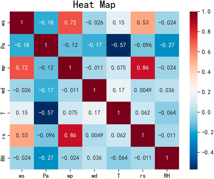
FIGURE 3. Pearson correlation coefficient heat map.

According to the thermal map, it can be seen that the two variables with the highest correlation with the final output wind power (wp) are wind speed (ws) and fan turbine speed (rs), and the correlation is 0.72 and 0.86, respectively. Therefore, this paper chooses these two variables as inputs to the LSTM model to predict the future wind power.

4.1 Abnormal data detection and cleaning

4.1.1 Raw data

Numbers 1, 2, and 3 correspond to the three units in the northwest power plant; 4, 5, and 6 to the center region; and 7, 8, and 9 to the coastline region in the raw data of nine units from three distinct wind farms. There are 10,000 samples chosen for each unit. In the data pre-processing stage, the link between power, wind speed, and fan speed is examined to pinpoint the location information of the anomalous data.

Figure 4 shows the distribution range of wind speed for 9 units. Among them, the wind speed is almost Normal distribution, and most of the points are concentrated in the wind speed range of (3–8) m/s. The points outside this range have a high probability of being abnormal data. For example, the data distributed around the wind speed of 0 m/s are called wind speed abnormal points, which have the characteristics of wind speed (cut in wind speed, power>0). Most of the power data are distributed at 0 and do not show Normal distribution, which also indicates that the power data collected by the SCADA system contains more abnormal data. The fan speed is mainly concentrated between 8 and 15, and we can speculate that there is a high possibility of abnormal data in fan speeds outside this range (see attached materials for statistics on power and fan speed).

FIGURE 4

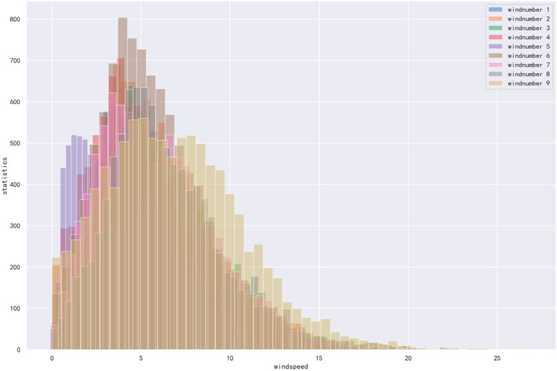
FIGURE 4. Wind speed statistics for 9 units.

It was discovered that each of the nine units had varying degrees of aberrant data through the visual inspection of the aforementioned individual factors. Therefore, in this paper, using Unit 1 as an example, the three-dimensional scatter plots of wind speed (x-axis), power (y-axis), and fan speed (z-axis) of Unit 1 are plotted. Results as shown in Figure 5. This is because it is necessary to analyze the combination of these three groups of characteristic variables in order to further analyze the causes of the abnormal data distribution.

The distinctive scatter plots can be loosely categorized into three groups, as can be seen in the image. The first category (in the yellow dashed box) is the anomalous data piled up at the bottom, which typically appears due to a communication or abandoned wind power limit anomaly; The reason for the appearance of discrete anomalies is typically Extreme weather, sensor failure, or signal propagation noise; the third category (in the orange dashed box) has a small amount of data scattered at the top, similar to the second category.

FIGURE 5

FIGURE 5. Unit 1 3D scatter diagram.

4.1.2 Abnormal data cleaning and ablationexperiments

The anomalous data should be removed because, based on the previous description and the analysis of the actual wind power plant power, wind speed, and wind turbine speed, they are not uniformly distributed in range and have a tendency to pile up at the bottom and show dispersion in the middle and top. This makes it difficult for a neural network to use timing logic to predict future wind power.

The ideal number of clusters is first determined using the Elbow approach. The degree of aberration is the squared distance error sum of the prime and sample points within each cluster, which is calculated using k-means to minimize the squared sample and prime error as the objective function. So, given a cluster, the tighter the cluster members are, the lower the degree of aberration, and the looser the cluster structure is, the greater the degree of aberration. The degree of aberration decreases as the category size increases, but for data with a certain level of differentiation, the degree of aberration improves significantly when a particular critical point is reached, then gradually declines Liu and Deng (2021). This critical point can be thought of as the point where clustering performance is best. Still using Unit 1 as an example, the Figure 6 shows the curve of Elbow method for Unit 1.

FIGURE 6

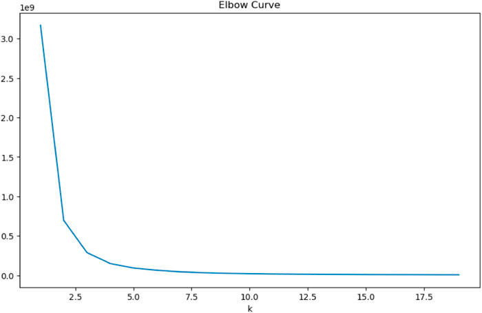
FIGURE 6. Unit 1Elbow method curve.

From the graph, it can be seen that the curve starts to smooth out at k = 2, and the distortion of the curve is greatly improved at k = 2.5. However, since k can only be obtained as an integer, k = 2 is chosen as the clustering number in this paper. The left half of Figure 7 shows the classified data. It can be seen that after clustering processing, the original windspeed-windpower-rotorspeed scatter plot is divided into two parts, one part (red) is stacked data, and the other side (yellow) is discrete data. According to the literature, K-means algorithm can handle data with high density, so this paper uses K-means to clean the above part of the data. Although DBSCAN algorithm is not effective in identifying stacked abnormal data, it does not need to set K value in advance and can improve cleaning efficiency. Therefore, DBSCAN is chosen in this paper to process the yellow abnormal data in the figure. In addition, set epsilon = 3 and minpts = 4 in DBSCAN. The right half of Figure 7 shows the 3D scatter diagram of 9 units after K-means and DBSCAN processing.

FIGURE 7

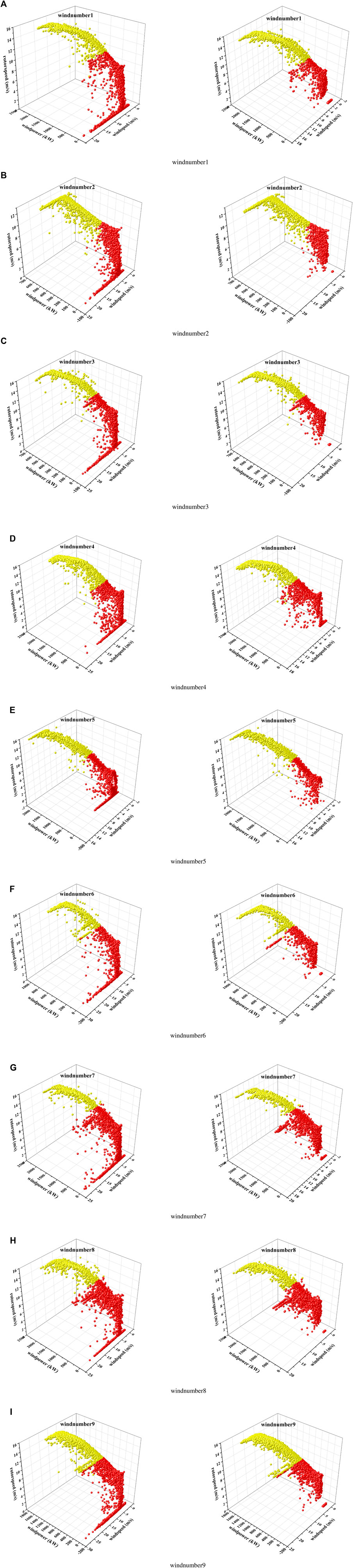
FIGURE 7. Comparison before and after data cleaning.

From the figure, it can be clearly seen that the K-means algorithm effectively eliminates the abnormal data accumulated in the power of 0, and also effectively deals with the discrete points of the red scatter points. For the yellow scattered points, because most of them are in the normal range, the cleaning effect is not obvious, but the problem of mistakenly deleting normal data is also avoided.

It is suggested that the error of the cleaning result and the standard power curve (Eq. 26), and the deletion rate (Eq. 27), the cleaning time (t) be used as the judging cleaning indexes to test the efficacy of the method in this study. The DBSCAN algorithm is designated as M1, K-means method as M2, and the algorithm in this paper as M3, and the outcomes are displayed in Table 1.

${AAD}_i=\frac{1}{N}{\displaystyle \sum _{j=1}^{N_i}}\left|P_i-P_{i,j}\right|(26)$

where AAD_i is the mean absolute error and root mean square error for the ith wind speed interval; N_i is the amount of data in the ith interval; P_i is the value of the standard power curve in the ith interval; and P_i,j is the ith power data in the ith interval.

$D\%=\frac{L_0-L_1}{L_0}\times 100\%(27)$

where, L₀ is the data volume of the original data set; L₁ is the data volume of the remaining data set after removing the abnormal data using the data cleaning method.

TABLE 1

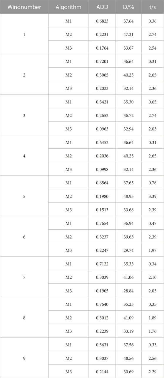
TABLE 1. Comparison of data before and after cleaning by KD algorithm.

The cleaning time is the quickest when only the DBSCAN method is used to clean the data, as its time complexity is typically less than O(N²), according to the data in the table. However, the deletion rate of this method is higher because the algorithm relies on the problem of incorrect identification of dense data with the setting of parameters as mentioned above in this paper, and the range of the threshold value can only be set smaller in order to obtain better cleaning effect of abnormal data, which in turn leads to more normal data being deleted by mistake.

Due to the mistaken deletion of normal data, the error between M1 cleaning results and the standard power curve is the largest among the three algorithms, Therefore, it is not feasible to use DBSCAN alone to handle different units in different regions on a large scale. Similar to the K-means method, which takes the longest to clean up and has a higher error, it has the issue of deleting a lot of data. The method used in this study has the lowest deletion rate and smallest inaccuracy of the three, demonstrating that classifying the original data and removing data from each class can optimize each algorithm’s benefits and more precisely identify the abnormal data.

In a comprehensive view, although the algorithm in this paper has the problem of insufficient recognition rejection efficiency, it has the lowest deletion rate under the same conditions, the least damage to the data integrity of the units, the smallest error between the cleaned results and the standard power curve, the most concentrated near the standard power curve, and high generality for different units.

4.2 Power prediction

The nine units cleaned from the prior data are input to the network to test the generalizability of the neural network model LSO-G-LSTM developed in this study, and the predicted power is output after parameter training to identify the best parameters.

First, set the parameters of each model. The total number of lions N = 20, the maximum number of iterations T_max = 100, and the number of adult lions β = 0.5 were set in LSO. Secondly, the initial learning rate of LSTM, LSO-LSTM and LSO-G-LSTM was set as 0.01, inputsize as 2-dimensional, hiddensize = 4,batchsize = 128; The initial values of LSO-G-LSTM network parameters λ, ω and γ are all 0. Finally, take the number 1 as an example to illustrate the variable parameters of the input model. Let this input be x_1t, according to the meteorological and unit characteristics analyzed above, only the wind speed and fan speed are selected as the input to the model, so the corresponding input variable matrix is $x_{1t}=[x_{1t}^{(1)},x_{1t}^{(2)}]$, and other units use the same method as the model input, where the number (1) and (2) in the upper right corner represent the wind speed and fan speed respectively. And ensure that multiple groups of experimental environment under the same condition.

Because the predicted wind power sequence in this paper is short-term, it will not last longer than 3 days. The sampling interval for each of the nine units is 10 min, and the predicted sample points for the predicted power for the upcoming 12 and 24 h are 72 and 144, respectively. Figure 8 displays the wind power forecast results for the upcoming 12 h for each of the nine units.

FIGURE 8

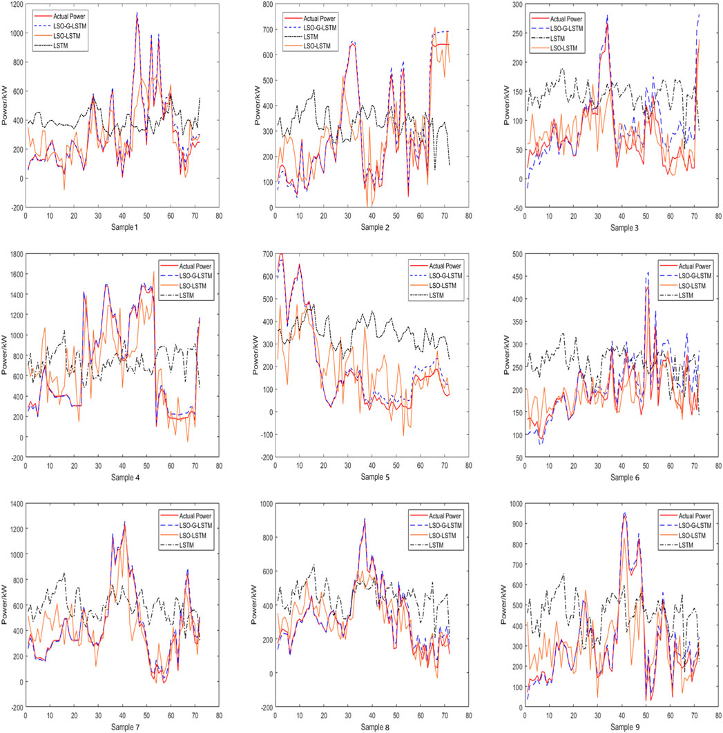
FIGURE 8. Power prediction curve of 9 units for the next 12 h.

Only a few data points from the nine sets of power estimates for the upcoming 12 h show that the LSTM neural network makes accurate predictions. This may be caused by the corruption of the time series of the original data after data cleaning, which also illustrates the shortcomings of LSTM in handling such data; Apart from samples 2, 6, 7, and 8, which are relatively close, there are large deviations from the initial data when predicting other units, and the phenomenon of overfitting appears at a later stage, which may be caused by the LSO algorithm entering a local optimum when training the LSTM parameters; The LSTM has significantly improved in terms of prediction accuracy after LSO optimization, and the prediction trend is roughly the same as the actual power; In this study, the model is able to concentrate on the impact of features on power after the addition of the GCT attention mechanism for LSTM. Additionally, after LSO training on three sets of GCT parameters, the prediction accuracy is significantly increased, and the curve fit is optimal, with deviation occurring only after about 50 samples. This study evaluates the prediction accuracy of several models using mean absolute percentage error (MAPE) and root mean square error (RMSE), which are defined as Equations (28)–(29), and the findings are displayed in Table 2. The more accurate the model prediction, the lower the value of MAPE and RMSE.

$MAPE=\frac{1}{n}{\displaystyle \sum _{i=1}^n}\frac{\left|x^{\prime }\left(i\right)-x\left(i\right)\right|}{x\left(i\right)}\times 100\%(28)$

$RMSE=\sqrt{\frac{1}{n}{\displaystyle \sum _{i=1}^n}{\left(x^{\prime }\left(i\right)-x\left(i\right)\right)}^2}(29)$

TABLE 2

TABLE 2. Error table of power prediction for the next 12 h by 9 units.

When estimating the wind power for the following 12 h, it can be noted that the MAPE and RMSE of the suggested models in this research are the smallest when compared to other models. Error (MAPE) of the nine units ranges from 9.156% to 16.38% and the root mean square error (RMSE) ranges from 1.028 MW to 1.546 MW. Taking the first unit as an example, compared with LSTM, xgBoost-LSTM, PSO-LSTM, Adaboost-LSTM and LSO-LSTM, MAPE increased by 61.36%, 46.36%, 50.94%, 30.80% and 21.27% respectively. RMSE increased by 45.23%, 43.93%, 28.79%, 28.83% and 7.558%, respectively. This demonstrates the LSO-G-LSTM model’s capacity to process vast amounts of data from numerous units in various regions and its ability to predict the power after 12 h more correctly and steadily. Additionally, Figure 9 displays each model’s prediction curves for the power of 144 data points throughout the course of the following day.

On the other hand, the LSO-LSTM model, which performs well in the 12-h prediction, shows a decline in the performance of the 24-h prediction and frequently fails to fit the power accurately. The model in this paper performs well in the 12-h prediction, but there are large deviations in the prediction of units 3 and 6, possibly due to the increase in step length and more data points. The models’ prediction errors are displayed in Table 3.

FIGURE 9

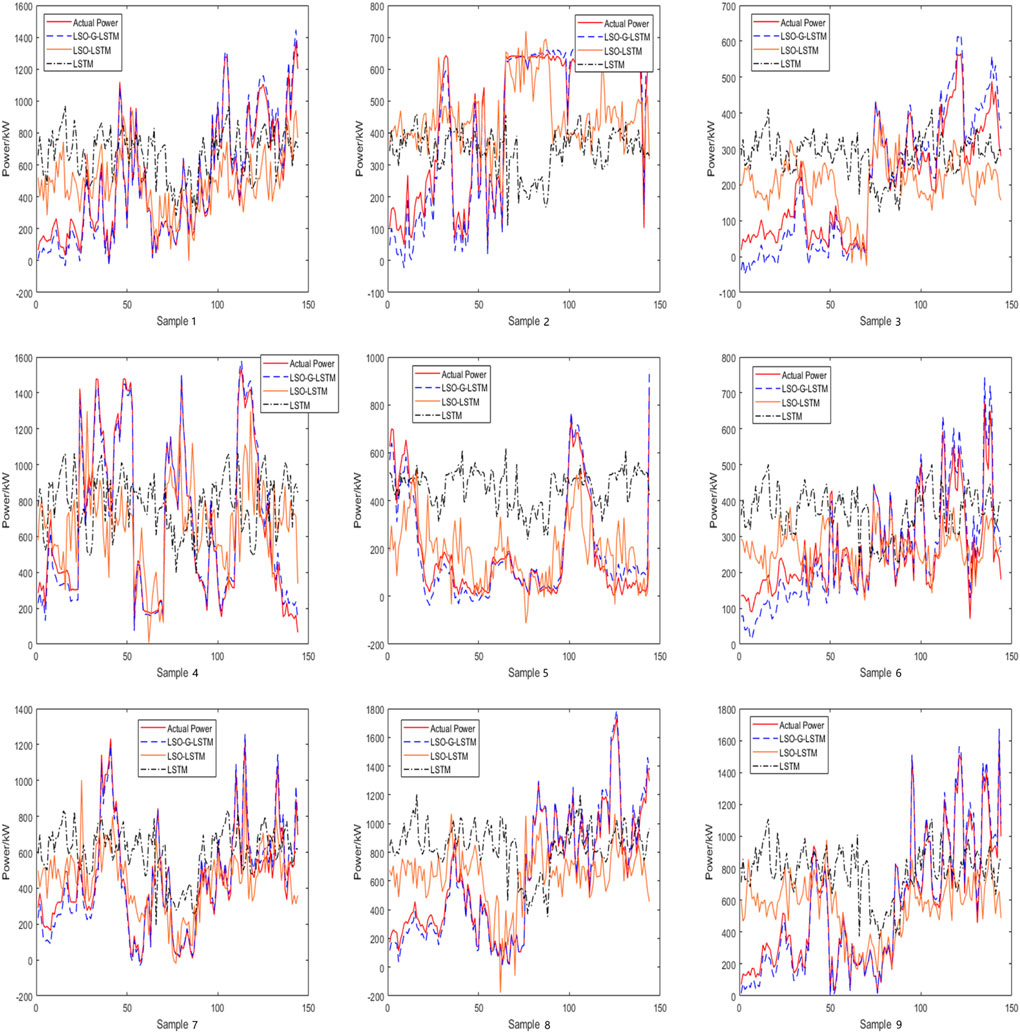
FIGURE 9. Power prediction curve of 9 units for the next 24 h.

TABLE 3

TABLE 3. Error table of power prediction for the next 24 h by 9 units.

According to the curves in the figure and the error statistics in the table, all models’ accuracy when performing multi-step prediction declines to varying degrees, but the error of the model developed in this research is still the smallest. It can be demonstrated that the LSTM is greatly enhanced by the addition of the GCT attention mechanism and is better suited for use as a model for short-term wind power prediction.

In addition, we should not ignore the influence of model output parameters on the prediction results. First of all, for the situation reflected by LSTM in the figure, we know that the model has an underfitting. Taking Group 1 as an example, the LSTM model is trained by calling the fit () function. This function returns a variable named. history, which contains loss and accuracy during model compilation. This information is displayed at the end of each epoch training session. For 12 h prediction, the total amount of data needed to be trained for each group of models is 9928, batchsize = 128, so the batch required for training is = 9928/16 = 621 (rounded up), and the hidden layer is defined as [LSTM:2× the number of layers by default 1, batchsize, each unit contains hidden units]. And output, (h_n, c_n), where output:LSTM output of the last hidden state, hn: the hidden state result of the last timestep, cn: the cell unit result of the last timestep. Table 4 shows the loss value and accuracy of training set parameters during 12 h short-term power prediction for 9 units.

TABLE 4

TABLE 4. LSTM model training set parameters.

According to Table 4, the epoch = 780 obtained when the LSTM model stops training. At this time, loss780 = 0.7234, accuracy780 = 0.6198, the values of loss1-loss780 decrease monotonically, while the accuracy1-accuracy780 increases monotonically. This indicates that there is still room for loss to decrease while accuracy has room for improvement at the end of the separate LSTM training. After retraining, it is found that the epoch stops when loss943 = 0.6751, accuracy943 = 0.8845, and accuracy943 = 0.8845. It is shown directly that the model falls into local optimality in the first training, and the model appears underfitting. For the LSO-LSTM model, after adding the LSO disturbance factors α_f and α_c, the model has not converged during training and the training will be stopped when the epoch = 1800, when loss 1800 = 0.1498 and accuracy 1800 = 0.8124. However, when the epoch = 1700, the accuracy 1800 = 0.8124. loss1700 = 0.2075, and accuracy1700 = 0.8724. It can be seen that when the epoch is reduced, the accuracy of the training model will increase; however, when the epoch = 1900 is continued, the loss and accuracy will decrease at the same time, indicating that the model is overfitting and it will be difficult for the model to converge. In most cases, the model can not fit the real value well, and the generalization ability is poor. With the epoch = 1265, loss1265 = 0.2627, and accuracy1265 = 0.9533, accuracy1265 can be set with the epoch = 1000 and 1100, and the loss will increase and the accuracy will decrease. With the epoch = 1300 and 1400, the loss will no longer decrease. The value of accuracy does not change. Combined with the curve in the figure above and the error value in the table, it indicates that the model has converged and does not fall into the local optimal.

The input data for the aforementioned tests are all of the predictions after K-means and DBSCAN cleaning, and they serve merely to demonstrate the success of the LSTM model improvement shown in this research. This research examines the errors of each model without rejecting the identification of anomalous data using the 12 h anticipated power as an example, as shown in Figure 10 in order to demonstrate the significance of data pre-processing.

FIGURE 10

FIGURE 10. Prediction error in the next 12 h before Data cleansing.

In addition, the errors of the model before and after data processing for the next 12 and 24 h are also compared, as shown in Figure 11.

FIGURE 11

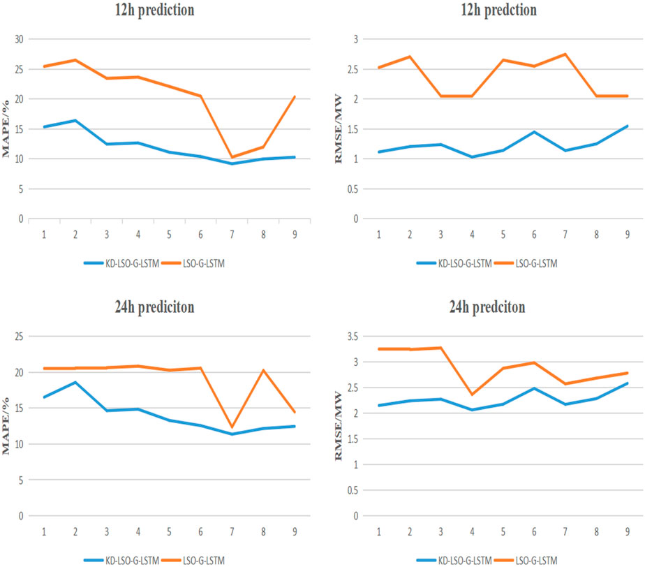
FIGURE 11. Error analysis of the model before and after data cleaning.

The error values are all increased to varying degrees, but the error increase of units 1, 2, 8 and 9 is larger, which also corroborates the hypothesis that the analysis of discrete abnormal data in Figure 7 has a greater impact on the prediction results. These results come from the prediction histogram of each model for the next 12 h without abnormal data detection and rejection. The errors of MAPE and RMSE predicted by LSTM for Unit 1 increased by 19.08% and 34.45%, respectively; those predicted by xgBoost-LSTM increased by 24.84% and 31.55%; those predicted by PSO-LSTM increased by 24.58% and 37.48%; those predicted by Adaboost-LSTM increased by 29.27% and 34.83%; those predicted by LSO-LSTM increased by 30.50% and 46.49%; and those predicted by the model in this These data also show how cleansing the raw wind power series is necessary for anomaly data analysis and identification.

Additionally, the figure supports the aforementioned conclusion. The red dash depicts the error indicators without data processing, whereas the blue dash shows the error indicators of each unit for the model’s 12 and 24 h wind power predictions in this research. The blue dash is consistently smaller than the red line for the future 12-h power prediction, but for the future 24-h prediction, both error values rise and the blue and red curves converge due to the future wind power’s instability and uncertainty as the prediction step increases. Nevertheless, when compared to other models and to itself both before and after cleaning the data, the KD-LSO-G-LSTM model suggested in this study produces the best prediction results.

5 Conclusion

In order to improve the accuracy of wind power prediction, this study proposed a short-term wind power prediction model of KD-LSO-G-LSTM based on abnormal data detection and cleaning. In the manuscript, the stability and universality of the algorithm were discussed by taking wind turbines in different regions of China as examples. Firstly, in the data preprocessing part, K-means and DBSCAN algorithm are combined to detect and clean abnormal data to improve the stability of prediction. Secondly, by combining GCT attention mechanism module with LSTM input parameters, a new feature vector is constructed to ensure the optimal feature selection for prediction. Finally, the lion pride algorithm is used to optimize the model to avoid its parameters falling into local optimality in the training process, and also to ensure that underfitting and overfitting will not occur in the prediction, so as to improve the prediction accuracy. The proposed algorithm fills the gap in anomaly data cleaning and prediction accuracy. Three sets of experiments were conducted in this section.

The first set is an ablation experiment for KD abnormal data cleaning algorithm, aiming to evaluate the effectiveness of combining the two algorithms for data cleaning. The error, deletion rate and cleaning time of the cleaning data of 9 units are evaluated, and the result proves the superiority of KD algorithm in removing abnormal data. The second experiment evaluated the error of different algorithms in predicting the same wind power. Through the prediction results of 12 and 24 h in the future, it can be seen that the accuracy and stability of the proposed algorithm in predicting the power of more units are the least error among all models. The third set of experiments verified the prediction errors of different models before and after data cleaning, aiming to show the necessity of abnormal data cleaning. The results also showed that the errors of the models with abnormal data processing were smaller than those without processing.

Combined with the results of the above three groups of experiments, the effectiveness and universality of KD-LSO-G-LSTM in short-term power prediction can be obtained. However, due to the elimination of the original data in this paper, the original time series is damaged, which makes the efficiency of such time-serial-dependent prediction models as LSTM decrease. In future work, we will consider adding some series reconstruction methods to improve its prediction efficiency. In addition, China has a vast territory and a large population, which has high requirements for the stability and safety of electricity consumption, and its dependence on this kind of new energy is increasing year by year. Therefore, the forecast results of only three regions cannot prove whether the study is equally applicable in other regions of China. Future prospects for this study therefore include evaluating the proposed method on larger data sets and over more areas to confirm the superiority of the proposed method for short-term wind power prediction.

Data availability statement

The raw data supporting the conclusions of this article will be made available by the authors, without undue reservation.

Author contributions

WX: Funding acquisition, Writing–review and editing. ZS: Writing–original draft. XF: Supervision, Writing–review and editing. YL: Writing–review and editing.

Funding

The authors declare financial support was received for the research, authorship, and/or publication of this article. This research was funded by: National Natural Science Foundation of China (U1802271), Research on Digital Protection and Heritage of Brown Culture in the Context of Sustainable Development” (2023YNMW010) of Yunnan Provincial People’s Committee.

Conflict of interest

The authors declare that the research was conducted in the absence of any commercial or financial relationships that could be construed as a potential conflict of interest.

Publisher’s note

All claims expressed in this article are solely those of the authors and do not necessarily represent those of their affiliated organizations, or those of the publisher, the editors and the reviewers. Any product that may be evaluated in this article, or claim that may be made by its manufacturer, is not guaranteed or endorsed by the publisher.

Supplementary material

The Supplementary Material for this article can be found online at: https://www.frontiersin.org/articles/10.3389/fenrg.2023.1268494/full#supplementary-material

References

Chandel, S., Murthy, K., and Ramasamy, P. (2014a). Wind resource assessment for decentralised power generation: case study of a complex hilly terrain in western himalayan region. Sustain. Energy Technol. Assessments 8, 18–33. doi:10.1016/j.seta.2014.06.005

CrossRef Full Text | Google Scholar

Chandel, S., Ramasamy, P., and Murthy, K. (2014b). Wind power potential assessment of 12 locations in western himalayan region of India. Renew. Sustain. Energy Rev. 39, 530–545. doi:10.1016/j.rser.2014.07.050

CrossRef Full Text | Google Scholar

Chen, Y., and Lin, H. (2022). “Overview of the development of offshore wind power generation in China,” in Sustainable energy technologies and assessments.

CrossRef Full Text | Google Scholar

Diaconita, A. I., Andrei, G., and Rusu, L. (2022). “An overview of the offshore wind energy potential for twelve significant geographical locations across the globe,” in Selected papers from 2022 7th international conference on advances on clean energy research (Energy Reports), 8, 194–201.

CrossRef Full Text | Google Scholar

Ding, Y., Chen, Z., Zhang, H., Wang, X., and Guo, Y. (2022). A short-term wind power prediction model based on ceemd and woa-kelm. Renewable Energy.

Google Scholar

Du, B., Huang, S., Guo, J., Tang, H., Wang, L., and Zhou, S. (2022). Interval forecasting for urban water demand using PSO optimized KDE distribution and LSTM neural networks. Applied Soft Computing 122, 108875–545.

CrossRef Full Text | Google Scholar

González-Sopeña, J., Pakrashi, V., and Ghosh, B. (2021). An overview of performance evaluation metrics for short-term statistical wind power forecasting. Renew. Sustain. Energy Rev. 138, 110515. doi:10.1016/j.rser.2020.110515

CrossRef Full Text | Google Scholar

Greff, K., Srivastava, R., Koutník, J., Steunebrink, B. R., and Schmidhuber, J. (2015). Lstm: a search space odyssey. IEEE Trans. Neural Netw. Learn. Syst. 28, 2222–2232. doi:10.1109/tnnls.2016.2582924

CrossRef Full Text | Google Scholar

Hahsler, M., Piekenbrock, M., and Doran, D. (2019). dbscan: fast density-based clustering with r. J. Stat. Softw. 91. doi:10.18637/jss.v091.i01

CrossRef Full Text | Google Scholar

Hamed, K. M., Soleimanian, G. F., Kambiz, M., and Amin Babazadeh, S. (2022). A New Hybrid Based on Long Short-Term Memory Network with Spotted Hyena Optimization Algorithm for Multi-Label Text Classification. Mathematics 10 (3), 488. doi:10.3390/math10030488

CrossRef Full Text | Google Scholar

Hui, H., Rong, J., and Songkai, W. (2018). Ultra-short-term prediction of wind power based on fuzzy clustering and rbf neural network. Adv. Fuzzy Syst. 2018, 9805748:1–7. doi:10.1155/2018/9805748

CrossRef Full Text | Google Scholar

Jin, X., and Han, J. (2021). “K-means clustering,” in Learn data mining through excel.

Google Scholar

Krishna, V., Mishra, S. P., Naik, J., and Dash, P. K. (2021). Adaptive vmd based optimized deep learning mixed kernel elm autoencoder for single and multistep wind power forecasting. Energy.

Google Scholar

Lee, S., Kim, K., Lee, M. S., and Lee, J. S. (2020). Recovery of inter-detector and inter-crystal scattering in brain pet based on lso and gagg crystals. Phys. Med. Biol. 65, 195005. doi:10.1088/1361-6560/ab9f5c

PubMed Abstract | CrossRef Full Text | Google Scholar

Li, H. (2022). “Short-term wind power prediction via spatial temporal analysis and deep residual networks,” in Frontiers in energy research, 10.

CrossRef Full Text | Google Scholar

Li, N., Wang, Y., Ma, W., Xiao, Z.-N., and An, Z. (2022). “A wind power prediction method based on de-bp neural network,” in Frontiers in energy research, 10.

CrossRef Full Text | Google Scholar

Liu, F., and Deng, Y. (2021). Determine the number of unknown targets in open world based on elbow method. IEEE Trans. Fuzzy Syst. 29, 986–995. doi:10.1109/tfuzz.2020.2966182

CrossRef Full Text | Google Scholar

Liu, Z., Hajiali, M., Torabi, A., Ahmadi, B., and Simoes, R. (2018). Novel forecasting model based on improved wavelet transform, informative feature selection, and hybrid support vector machine on wind power forecasting. J. Ambient Intell. Humaniz. Comput. 9, 1919–1931. doi:10.1007/s12652-018-0886-0

CrossRef Full Text | Google Scholar

Lu, R., Zhu, J., Qian, X., Tian, Z., and Yue, Y. (2021). Scaled gated networks. World Wide Web 25, 1583–1606. doi:10.1007/s11280-021-00968-2

CrossRef Full Text | Google Scholar

Malakouti, S., Ghiasi, A., Ghavifekr, A. A., and Emami, P. (2022). Predicting wind power generation using machine learning and cnn-lstm approaches. Wind Eng. 46, 1853–1869. doi:10.1177/0309524x221113013

CrossRef Full Text | Google Scholar

Meka, R., Alaeddini, A., and Bhaganagar, K. (2021). A robust deep learning framework for short-term wind power forecast of a full-scale wind farm using atmospheric variables. Energy 221, 119759. doi:10.1016/j.energy.2021.119759

CrossRef Full Text | Google Scholar

Nielson, J., Bhaganagar, K., Meka, R., and Alaeddini, A. (2020). Using atmospheric inputs for artificial neural networks to improve wind turbine power prediction. Energy 190, 116273. doi:10.1016/j.energy.2019.116273

CrossRef Full Text | Google Scholar

Ramasamy, P., Chandel, S., and Yadav, A. (2015). Wind speed prediction in the mountainous region of India using an artificial neural network model. Renew. Energy 80, 338–347. doi:10.1016/j.renene.2015.02.034

CrossRef Full Text | Google Scholar

Schubert, E., Sander, J., Ester, M., Kriegel, H., and Xu, X. (2017). Dbscan revisited, revisited. ACM Trans. Database Syst. (TODS) 42, 1–21. doi:10.1145/3068335

CrossRef Full Text | Google Scholar

SheenaKurian, K., and Mathew, S. (2023). High impact of rough set and kmeans clustering methods in extractive summarization of journal articles. J. Inf. Sci. Eng. 39, 561–574. doi:10.6688/JISE.20230539(3).0007

CrossRef Full Text | Google Scholar

Uddin, Z., and Sadiq, N. (2022). Method of quartile for determination of weibull parameters and assessment of wind potential. Kuwait J. Sci. doi:10.48129/kjs.20357

CrossRef Full Text | Google Scholar

Wang, S., Ji, T., and Li, M. (2020). “Power load forecasting of lssvm based on real time price and chaotic characteristic of loads,” in Information security practice and experience, 2172–2178.

CrossRef Full Text | Google Scholar

Wang, Y., Xue, W., Wei, B., and Li, K. (2022a). An adaptive wind power forecasting method based on wind speed-power trend enhancement and ensemble learning strategy. J. Renew. Sustain. Energy 14. doi:10.1063/5.0107049

CrossRef Full Text | Google Scholar

Wang, Y., Zhang, Y., Liu, H., Wu, L., Yang, W., and Liang, K.-F. (2022b). “Wind turbine abnormal data cleaning method considering multi-scene parameter adaptation,” in 2022 asian conference on Frontiers of power and energy (ACFPE), 292–297.

CrossRef Full Text | Google Scholar

Wisdom, U., and Yar, M. (2021). Data-Driven Predictive Maintenance of Wind Turbine Based on SCADA Data. IEEE Access 9, 162370–162388. doi:10.1109/ACCESS.2021.3132684

CrossRef Full Text | Google Scholar

Wu, Z., and Wang, B. (2021). An ensemble neural network based on variational mode decomposition and an improved sparrow search algorithm for wind and solar power forecasting. IEEE Access 9, 166709–166719. doi:10.1109/access.2021.3136387

CrossRef Full Text | Google Scholar

Wu, Y., and Gao, J. (2023). AdaBoost-based long short-term memory ensemble learning approach for financial time series forecasting. Current Science 115, 159–165. https://www.jstor.org/stable/26978163

Google Scholar

Yang, S., min Yuan, A., and Yu, Z. (2022). A novel model based on ceemdan, iwoa, and lstm for ultra-short-term wind power forecasting. Environ. Sci. Pollut. Res. 30, 11689–11705. doi:10.1007/s11356-022-22959-0

PubMed Abstract | CrossRef Full Text | Google Scholar

Yuan, X., Chen, C., Jiang, M., and Yuan, Y. (2019). Prediction interval of wind power using parameter optimized Beta distribution based LSTM model. Applied Soft Computing 82, 105550. doi:10.1016/j.asoc.2019.105550

CrossRef Full Text | Google Scholar

Zhang, X., Li, H., Zhu, B., and Zhu, Y. (2020). Improved ude and lso for a class of uncertain second-order nonlinear systems without velocity measurements. IEEE Trans. Instrum. Meas. 69, 4076–4092. doi:10.1109/tim.2019.2942508

CrossRef Full Text | Google Scholar

Zhang, Y., Zhu, S., Yu, C., and Zhao, L. (2022). Small-footprint keyword spotting based on gated channel transformation sandglass residual neural network. Int. J. Pattern Recognit. Artif. Intell. 36, 2258003:1–2258003:16. doi:10.1142/s0218001422580034

CrossRef Full Text | Google Scholar

Zhao, M., Wang, Y., Wang, X., xia Chang, J., Zhou, Y., and Liu, T. (2022). “Modeling and simulation of large-scale wind power base output considering the clustering characteristics and correlation of wind farms,” in Frontiers in energy research, 10.

CrossRef Full Text | Google Scholar