 Zhenbo Niu
 Chao Zheng
95% of researchers rate our articles as excellent or good
Learn more about the work of our research integrity team to safeguard the quality of each article we publish.
Find out more
ORIGINAL RESEARCH article
Front. Energy Res. , 23 January 2024
Sec. Smart Grids
Volume 11 - 2023 | https://doi.org/10.3389/fenrg.2023.1267303
This article is part of the Research Topic Planning, Operation and Control of Modern Power System with Large-scale Renewable Energy Generations, volume II View all 15 articles
Based on real-time access to response information on wide-area tributaries, in order to assess the system stability more quickly, this paper combines the simplified branch transient transmission capability (sBTTC) index and the largest Lyapunov exponent (MLE). An online identification method for transient power angle stability is proposed. Firstly, the method is based on a two-machine system to study the consistency of the power angle difference between the two ends of the critical branch and the change of the phase difference of the fleet. Secondly, the transient power angle stability problem is transformed into the MLE analysis problem according to the change rule of sBTTC index of the key branch. Then, by combining the characteristics of MLE curve and sBTTC index curve, the transient power angle stability criterion is given. Finally, the proposed method is verified and analysed by simulation examples. The method has strong industrial applicability because it does not need system model, the information source is easy to measure, it has strong anti-noise ability, and it overcomes the defect of the traditional method that needs to set a fixed symbolic observation window.
Transient angle stability assessment constitutes a crucial research aspect for ensuring the secure and stable operation of power systems (Wang and Wu, 1991; Sun et al., 2006; Chen et al., 2017). In recent years, the introduction of new energy sources and power electronic devices into the power grid, alongside the implementation of extra-high voltage direct current transmission projects, has significantly altered the stability profile of the power grid. (Kundur et al., 2004; Liu T et al., 2023; Andersson et al., 2005). Therefore, accurate identification of power system stability patterns is an important prerequisite for effective emergency control.
At present, for the system generator rotor angle stability problem has been carried out by scholars a lot of research. In terms of the out-of-step criterion based on generating unit information, the most ahead and lagging unit pairs are captured, and the equal area criterion is applied to quickly discriminate the stability (Paudyal S et al., 2010). Stability criterion is constructed based on single machine energy function and group pair energy function (Mu et al., 1993; Gou Jing et al., 2015; Gou J. et al., 2015) devises a transient stability discrimination index set based on the energy function of generator pairs and utilizes this index set for stability discrimination. Additionally, (Xie et al., 2006), leverages the concavity and convexity characteristics of the phase trajectory of equivalent units to accomplish stability discrimination through unit grouping. System stability is assessed based on the distance of the state point from the boundary of the dynamic security domain (Zeng et al., 2018; Liu et al., 2018).
The above method of stability determination based on unit response information needs to involve the whole network units and the required information is difficult to measure. The stability judgement relies on the generator grouping result, which is difficult to apply to the new type of power system. (Xue et al., 1989; Xue and Xue, 1999).
Based on the measurement information provided by wide area measurement system (WAMS) (Qin et al., 2008), the mode of “real-time decision-making, real-time control” can accurately and efficiently identify the system stability, effectively reduce the chain reaction caused by large disturbances, and have important significance for the safe and stable operation of the power grid (Liu et al., 2013; Tang, 2014; Lin et al., 2016). The research methods based on the network response information include transient energy function method, phase trajectory characteristic analysis method, artificial intelligence method (Tian and Zhao, 2023) and so on. Among them, the Maximum Lyapunov Exponential analysis method based on chaos theory has become research hotspot (Ravikumar and Khaparde, 2018). The concept of MLE was firstly applied to the power system transient stability discrimination, and the positive and negative signs of MLE were used to predict whether the power system was destabilized or not (Liu C W et al., 1994). A method for calculating the MLE and then determining the transient stability of the system based on the system model is proposed (Yan et al., 2011). Combining the mathematical model of the system with the definition of MLE, the stability of the system is monitored by calculating the Lyapunov exponential spectrum (Wadduwage D P et al., 2013). The above methods for calculating MLE have many disadvantages, such as being dependent on the system model, requiring high-dimensional phase space reconstruction, being extremely computationally complex, and being unfavorable for online engineering applications. The transient angle stability of the system is monitored by solving the MLE for a time series window of relative angles of all generators of the system. The algorithm requires only simple arithmetic calculations and is computationally fast (Dasgupta et al., 2013). By presetting the time observation window of MLE symbols, an MLE calculation method without system model is proposed (Dasgupta et al., 2015). However, the fixed time observation window cannot adapt to the variable fault disturbances, and it is necessary to observe the generating units of the whole network, which involves a huge amount of information. For this reason, a transient stability monitoring method based on the dynamic characteristics of the trajectory MLE of the key unit pair is proposed by finding the key unit pair, but the generator angle information is difficult to be measured directly (Huang et al., 2020). By analyzing the machine-end voltage information that can be measured directly, the least squares method is used to improve the calculation method of MLE, and the system instability criterion is given by combining the characteristics of the MLE curve (Shaopan et al., 2017). However, relying only on any one-dimensional end-voltage response sequence as the analysis data lacks reliability, and it is difficult to locate the key information sources.
Building upon prior research, this paper introduces a Maximum Lyapunov Exponent (MLE) transient stability analysis method based on the key branch response information. The approach involves several key steps. Firstly, this paper analyzes the characteristics of network node phase with clustering attribution in unstable system. The angle difference between the nodes at both ends of the key branch is consistent with the change of the angle difference between the leading and lagging clusters. Secondly, in this paper, the transient angle stabilization problem is transformed into a problem of MLE curve trajectory analysis of sBTTC exponential curves. In both stable and unstable forms, this paper analyses the MLE key properties of the sBTTC exponential response time series using the MLE solution mechanism. Combining the crucial attributes of sBTTC and MLE, by optimizing the initial time window and the maximum observation time window of the MLE method, this paper proposes a new transient stability judgement method based on the disturbed response information of the key branch. Finally, for a typical 39-node system and a real AC-DC hybrid grid, this paper verifies the validity of the criterion by simulation.
In the typical model of a single machine infinity system shown in Figure 1, Es and δ represent the terminal voltage and angle of the oscillating unit. Er denotes the terminal voltage of the reference unit. X signifies the total reactance between the oscillating unit and the reference unit.

FIGURE 1. Typical model for angle stability analysis.
Point “m” represents an any measurement node associated with the position factor λm. The branch current and voltage vectors at node “m” are denoted by Eq. 1 and Eq. 2 respectively.
Substituting Eq. 1 into Eq. 2 yields Eq. 3, as follows
Consequently, the angle information at point “m” is expressed in Eq. 4.
Based on Eq. 4, it is evident that the phase θm of the node “m” relies on the position factor λm and the angle δ. To delve deeper into the correlation between θm, λm, and δ, the single machine infinity system model shown is established in Figure 2. X10 = 0.04pu, X12 = X60 = X45 = 0.004pu, X34 = X56 = 0.008pu, X23 = 0.012pu. The actual active power output of generator G1 is 100pu. The position factor λ2-λ6 of nodes B2-B6 correspond to [0.9, 0.6, 0.3, 0.1] respectively.
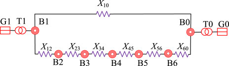
FIGURE 2. The single machine infinity system model.
At 1 s, a three-phase ground short-circuit fault occurs on the front side of the B1-B0 branch. In the case of system transient stability and transient instability, the fault clearing time is set to 0.06 s and 0.08 s respectively. In the example of system instability, the curve of generator angle and phase change of each node is shown in Figure 3.
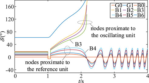
FIGURE 3. The curve of generator angle and phase change of each node.
As depicted in Figure 3, when angle instability occurs in the system, depending on the electrical distance to the reference unit, the phase of each node will be characterized by subgroup attribution. Using the electrical midpoint as a dividing line, Nodal phases close to the oscillating unit will tend to be close to the angle of the oscillating unit, while nodal phases close to the reference unit will be attributed to the angle of the reference unit. Therefore, the nodes in the network are consistent with the angle variation characteristics of the ahead and behind generator group. They all have the property of subgroup attribution. Within the B3-B4 branch comprising two nodes, the phase of the B3 node follows the same trend as that of the swing unit, and the phase of the B4 node follows the same trend as that of the reference unit. The phase difference between the B3-B4 branch and the angle of the unit always shows the trend of increasing in the same direction. Therefore, the B3-B4 branch is the key branch of the system, which can characterize the angle stability level of the system.
(Zheng et al., 2021a) defines an sBTTC index that monotonically represents the system stability condition based on wide-area branch response information. Based on this, Eq. 5 represents the simplified sBTTC index. The deterioration of system stability is reflected by setting a stability threshold.
Where: Uim and Uin represent the node voltage amplitude at the two ends of the i branch, respectively. Δ θ signifies the difference in the mode value of the node voltage vector at the two ends of the i branch.
In the destabilized system, the phase difference between the nodes at the two ends of the key branch shows a continuous increase and tends to be unbounded, while the voltage product keeps decreasing. This characteristic is reflected in Eq. 5, which shows that the phase difference between the two ends of the branch is 180° when the sBTTC index drops to 0, indicating system instability. During the initial descent phase of the sBTTC index, the sBTTC index values of all observed branches in the network are ordered from smallest to largest. According to Eq. 6, the key branch k has the smallest index value, and the candidate the key branch clusters have the next smallest index value. Additionally, the branch droop voltage coefficient ξv is introduced and combined with the branch droop voltage coefficient located within the interval [1,2] to distinguish the key branches (Zheng et al., 2021b; Zheng et al., 2022). Meanwhile, in order to improve the accuracy of discriminating the key branch, the branch droop voltage coefficient ξv is introduced and combined with the branch droop voltage coefficient located in the interval [1,2] for discrimination (Zheng et al., 2021a; Zheng et al., 2022).
When a system generator destabilisation occurs, at least one branch exists in the network. The phase difference between the nodes at the ends of this branch is consistent with the change in the power angle difference between the overrun and lagging units, and the centre of oscillation is located here. Among the AC lines in the whole network, the key branches have the weakest stability performance. The dynamic response process of sBTTC index of the key branch can directly reflect the transient angle stability of the whole system.
The sBTTC exponential variation curves for the key branch B3-B4 are illustrated in Figure 4 for the single machine infinity system in Section 2 under both the instability and stability cases.
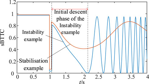
FIGURE 4. sBTTC curve for branch B3-B4.
The sBTTC exponential curve of branch B3-B4 is transformed to the sBTTC-d (sBTTC)/dt plane as shown in Figure 5. Calculate d (sBTTC)/dt as in Eq. 8:
where d (sBTTC)/dt and sBTTC(m−1)Δt,i represent the sBTTC index values of branch i at time instances mΔt and (m−1) Δt, respectively.
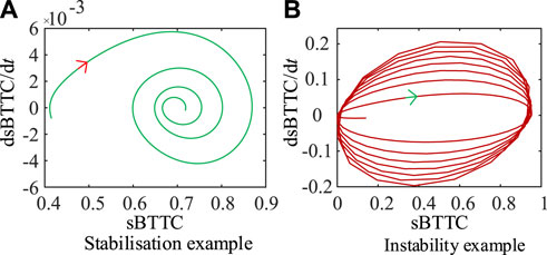
FIGURE 5. sBTTC-d (sBTTC)/dt curves for branch B3-B4.
As can be seen from Figure 5A, if the system transient angle is stability, the trajectory of sBTTC-d (sBTTC)/dt curve will gradually converge to a stable point, at which time the value of sBTTC-d (sBTTC)/dt is close to zero; from Figure 5B if the system transient angle is instability, the curve of sBTTC-d (sBTTC)/dt will be diverging around the zero axis, and cannot be converted to a stability equilibrium point. Therefore, the system angle stability analysis problem can be transformed into the problem of whether the sBTTC exponential curve can converge to a certain point. With the help of MLE, it can be used to determine the motion behavior of the power system; a negative MLE characterizes the convergence of trajectories, which represents the stability of the power system; a positive MLE characterizes the divergence of trajectories, which represents the instability of the power system.
The computations of MLE can be divided into those based on a system model and those that do not based on a system model. The PMU can measure the response information of the system, which facilitates the calculation of MLE without the need for a system model.
In Figure 6, the dynamic system observation trajectory is L. M is the original trajectory. N is the neighboring trajectory. M0, and N0 the starting points of the original and neighboring trajectories, respectively. Similarly, Mq and Nq stand as the reference points for the original and neighboring trajectories, while Mq+i and Nq+i represent the i point after the respective reference points.
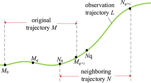
FIGURE 6. Observation trajectory.
The system sampling interval is Δt. At the moment iΔt, the logarithmic Euclidean distance curve lgL between the original and neighbouring trajectories is calculated as in Eq. 9.
As shown in Eq. 10, the MLE of the system at the moment iΔt is solved approximately using the MLE definition.
Eq. 10 only considers the resultant information of two points. In order to study the point-to-point transition process on the trajectory, it is necessary to use K data on the observation curve L as the initial time window. This necessitates satisfying the condition: ε1<‖LkΔt–L(k−1)Δt‖< ε2, where
The MLE method is used to determine the convergence of the curves. During the angle instability of the system, since the wide-area measurement system cannot directly measure the generator angle, it is necessary to find a suitable reference machine in order to effectively analyse the generator angle change curve. Therefore, the MLE analysis using the key branch sBTTC index time series as an observation has the following advantages:
(1) The branch sBTTC index takes the wide-area branch response information as the signal source, which can be obtained directly by the synchronous phase measurement unit (PMU). Compared with the traditional method (using the rotor angle of the most advanced generator as the information source), the MLE analysis of branch sBTTC index has the advantage of easy access to the information source.
(2) The branch sBTTC index has the property of monotonically decreasing with deterioration of stability properties. However, it is not possible to determine whether the system has crossed the unstable equilibrium point. The MLE analysis of the sBTTC index curve and the joint judgement of stability with the sBTTC index can determine the stability level of the system more quickly.
(3) The MLE method must select one-dimensional time series observations for phase space reconstruction in the N-dimensional dynamic system. Based on the sBTTC method, the key branch can be accurately located, and the system can be analysed in terms of stability preservation and dimensionality reduction.
(4) The MLE method can only calculate the MLE sign at a specific moment to reflect the eigenvalue sign at infinite moments. The sBTTC method can determine the optimal observation time window for the MLE method. The time window can be adjusted adaptively and is suitable for a variety of fault situations.
The selection of the initial time window requires ensuring that the distance change between the original and neighboring trajectories exhibits clear dynamic characteristics. In Section 3.1.2, the sBTTC-d (sBTTC)/dt plane trajectories have obvious dynamic convergence or divergence characteristics at the beginning. Both d (sBTTC)/dt and lgL, as calculated by Eq. 8 and 9 respectively, closely relate to the disparity between two points along the trajectories. Therefore, the beginning stage of original and neighbouring trajectory calculation also has obvious dynamic characteristics. In this paper, the initial value of the initial time window is chosen as the initial moment of the MLE calculation.
To examine the impact of different initial time window lengths on the MLE-t curve, we conducted calculations for two scenarios: M = 5 and M = 50, focusing on the stability and destabilization cases of a two-machine system. The resulting MLE-t curves for the sBTTC indices of key branches B3-B4 are presented in Figures 7A, B.

FIGURE 7. MLE-t curves for different initial time windows.
Under the stability and instability calculations for the stand-alone system, in order to analyse the effect of the selection of the initial time window length on the MLE-t curves, the initial window length M = 5 as well as M = 50 is set for the calculation. Figure 7 demonstrates the MLE-t curves for the sBTTC index of the B3-B4 key branch.
From Figure 7, the MLE-t curve can be divided into four phases:
(i) Initial stage: marked by significant fluctuations occurring in a brief span of time.
(ii) Descending stage: wherein the MLE-t curve consistently declines.
(iii) Oscillating stage: characterized by a continuous, periodic oscillation pattern in the MLE-t curve.
(iv) Stable stage: where the MLE-t curve eventually converges towards a stable value.
In the stability and instability cases, both M = 5 and M = 50 have no effect on the final sign of the MLE-t curve. Regardless of the length of the initial time window, the MLE-t curve eventually tends to be negative in the instability case and positive in the stability case. In this paper, the initial time window length M is taken as shown in Eq. 12, which can be adapted to systems of different sizes.
Where: nbus denotes the number of system nodes, and int represents upward rounding.
Maximum Lyapunov Exponent to discriminate the stability of the system needs to judge the final sign characteristics of the MLE. A time observation window of finite window length is usually predefined. The optimal time window depends on many factors and is difficult to determine. Theoretically, the length of the observation window tends to infinity to reflect the final MLE of the system. However, it is impossible to calculate the MLE at infinite moments due to the limitation of practical computational conditions.
If the optimal time observation window is too long, it may lead to the instability system crossing the unstable equilibrium point long time ago, and then the control action is implemented too late; if the optimal time observation window is too short, it may lead to the observation window not reflecting the final situation of the MLE-t curve, and then there is a misjudgment.
The sBTTC index can reflect the system stability level. Therefore, the initial moment of the optimal time window in this paper is set as the beginning moment of the initial decline phase of the sBTTC index, and the ending moment is the end moment of the initial decline phase of the sBTTC index. The dynamic observation time window set in this paper can be adapted to a variety of fault scenarios and can effectively discriminate the final sign of MLE.
It should be noted that, under the complex multivariable system, if the MLE sign is clear within the optimal time window, the observation of the MLE curve does not need to wait until the end of the optimal time window. On the contrary, if the MLE curve within the observation window has not entered the oscillation phase, the MLE sign cannot be determined. In this case, it is necessary to observe the value of the sBTTC index at the end of the dynamic observation window to make a determination.
The aim is to reduce the effect of noise on the signal and improve the curve smoothness. This paper employs the Savitzky-Golay filtering signal processing technique to refine the calculation of the MLE.
Following the fault occurrence, the sBTTC index information of the key branch can be acquired through real-time PMU sampling. Utilizing Eq. 9, the logarithmic Euclidean variation distance of the sBTTC index generates a one-dimensional signal sequence of length N, denoted as lgL lgL = [lgL1, lgL2, …. LgLN]. To apply the filter, a window of length 2d + 1 is selected, resulting in the subsequence lgL_w = [lgLn-d, …lgLn, …lgLn+d], where lgLn serves as the central data. The order of polynomial fitting is set as p, and the window’s subsequence is represented by the fitting polynomial, as shown in Eq. 13:
Where: X is the relative position within the window, i.e.,
The objective function corresponds to the squared discrepancy between the subsequence fitting polynomial and the original signal subsequence, expressed as shown in Eq. 14.
The fitting polynomial coefficients, denoted as
After the system is disturbed, the MLE curve of the sBTTC index of the key branch will show certain dynamic characteristics. This characteristic can reflect the system stability. Therefore, the MLE dynamic characteristics of this response trajectory are studied to discern the system stability in time.
In Section 2, the MLE-t curve of the response time series for the sBTTC index of the key branch B3-B4 is depicted in Figure 8, utilizing the stabilisation and instability examples of the two-machine system. The point B moment corresponds to the end moment of the initial descending phase of the sBTTC index, signifying the conclusion of the observation window.

FIGURE 8. MLE-t curves of key branches in Double-machine.
As can be seen from Figures 8A, B, the MLE-t curves of the stabilisation and instability cases continue to decrease after an initial fluctuation phase, then oscillate and oscillate continuously, and finally equilibrate at a constant value. During the process from the beginning of the calculation to point B, the apex of the first swing of the MLE curve is less than zero in the stabilisation case, while the apex of the first swing of the MLE curve is greater than zero in the destabilisation case. Therefore, the stability of the system can be determined by observing the characteristics of the first swing vertex of the MLE-t curve.
The application architecture for the joint judgement of stability between the sBTTC method and the MLE method can be divided into three modules:
(1) Data preparation module: This module utilizes the wide-area measurement system to gather voltage and phase data from the nodes at both ends of the branch.
(2) Calculation module: In this module, the following steps are performed:
i) The sBTTC index of the observed branch is computed using Eq. 5, and the key branch is identified through Eq. 6 and 7. The response time series of the sBTTC index for the key branch, denoted as sBTTC = [sBTTC1, sBTTC2, … , sBTTCn], is obtained, where n represents the number of sampling points. The phase space dimension of the key branch response information is one, implying that the MLE is calculated for a single curve. ii) M initial data points are selected from the sBTTC sequence, satisfying the condition ε1<‖LmΔt–L(m−1)Δt‖< ε2, where
(3) Stability analysis module: The system stability is discriminated according to the different characteristics presented by the MLE curve in the initial decline stage of the sBTTC index. Considering the timeliness of the system stability monitoring and the reduction of the false judgement rate, combined with the feature that the sBTTC index can reflect the deterioration of the system stability, the system stability level can be jointly discriminated by Eq. 15. Here, tc denotes the moment corresponding to the first peak vertex of the MLE curve, and εLth represents the threshold value set for the sBTTC index.
The transient stability analysis framework based on the MLE index and sBTTC index trajectory is depicted in Figure 9.
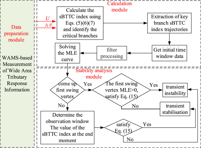
FIGURE 9. Flowchart of the framework.
The transient stability simulation calculation tool BPA is used to simulate the standard arithmetic case of a 10-machine, 39-node system. The disturbance response information is simulated as WAMS measurement data. The transient stability monitoring simulation calculation is carried out with a simulation step size of 0.01 s, for example,. sBTTC index threshold value εLth is set to 0.8.
A three-phase grounded short-circuit fault occurs on the front side of the bus16-bus17 branch at 0.2 s. The fault removal moment is set to 0.4 s. The system is transiently stable. The sBTTC index of the wide-area branch circuit based on WAMS measurement is shown in Figure 10.
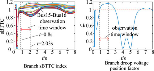
FIGURE 10. sBTTC index vs. dropout voltage position factor.
In Figure 10A, it is evident that the sBTTC index experiences the initial decline phase from t = 0.8 s to t = 2.03 s, which represents the MLE observation time window. Within this window, the bus15-bus16 branch exhibits the lowest sBTTC index value. The droop voltage position coefficient of this branch is illustrated in Figure 10B, and it satisfies the conditions stated in Eq. 7, confirming its key ity.
Next, the MLE curve of the sBTTC index trajectory for the bus15-bus16 branch is determined and depicted in Figure 11. At 1.33 s, the MLE curve exhibits its first swing vertex with a negative sign, while the value of the sBTTC index at that moment is 0.88, which is greater than the threshold value of 0.8 set previously. Based on these observations, we can conclude that the system is in a state of transient stability.

FIGURE 11. MLE-t curve under the destabilisation case.
At 0.2 s, a three-phase grounded short-circuit fault emerges on the front side of the bus16-bus17 branch, with the fault removal scheduled for 0.6 s. Consequently, the system experiences a single-swing destabilisation. In Figure 12, we observe the response curves of the generator angle and the entire network node voltage for the node system, with G30 serving as the reference machine.
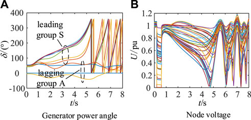
FIGURE 12. Transient response curve of 39-node system.
Figures 12A, B clearly indicates that the generator angle loses synchronisation after the fault, leading to a significant decline in node voltage, followed by continuous periodic oscillations. The system units divide into two groups: the leading group S, comprising 6 generators, and the lagging group A, comprising the remaining 4 generators, represented as S = {G31, G32, G33, G34, G35, G36} and A = {G30, G37, G38, G39}, respectively.
Upon calculating the sBTTC indices of the branches based on the disturbed response information and identifying the key branches, we assess whether their branch droop voltage location coefficients fall within the interval [1, 2], as depicted in Figure 13.
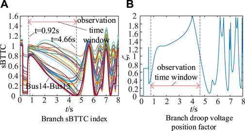
FIGURE 13. sBTTC index vs. dropout voltage position factor.
From Figure 13A, we can observe that within the time frame of 0.92 s–4.66 s, the branch sBTTC index consistently decreases to a value of zero. Throughout this process, the Bus14-Bus15 branch maintains the minimum sBTTC index value, and the branch footing voltage is situated atop this branch, confirming it as the key branch of the system.
Subsequently, we obtain the sBTTC index traces of the key branch and compute the MLE curve, as shown in Figure 14. Also, the MLE calculation curves for the traditional method of obtaining the most overrun unit G35 are given in Figure 14 (Dasgupta et al., 2015).
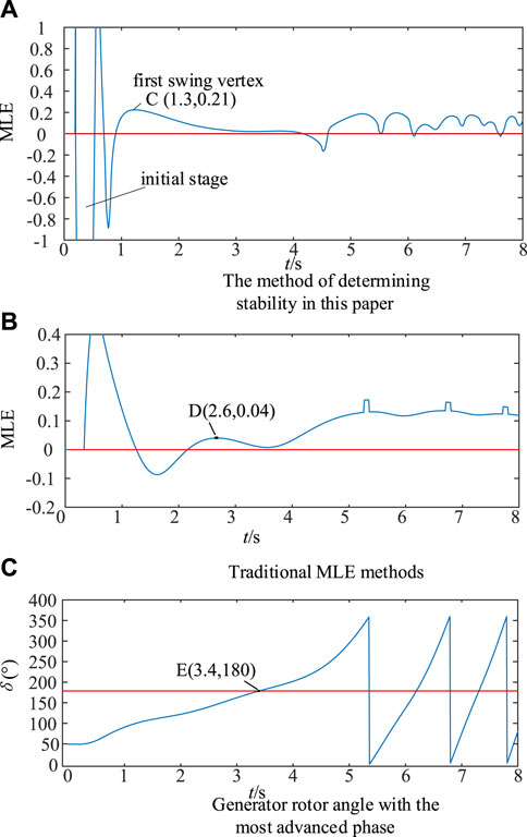
FIGURE 14. MLE-t curve under the destabilisation case.
In Figure 14A, the system stability is discriminated using the method proposed in this paper. The initial phase of the MLE-t curve is not given due to the large fluctuation, and the oscillation phase has long entered in the observation window. The first swing vertex of the MLE curve can be detected quickly at point C, and the value of the first swing vertex is 0.21. The value of the sBTTC index at this moment is 0.71, which is smaller than the set threshold value of 0.8. Therefore, this paper determines that the system is unstable for 1.3 s, and the maximum relative angle difference of the generator at this time is 1.91 rad.
In Figure 14B, the traditional method is used to calculate the MLE and determine the stability of the system. If the observation window is set to 3 s, the MLE sign can be determined to be positive at 2.6 s, and then the system is judged to be unstable. If the observation window is set too short, such as 2 s, the system will be misjudged as stable.
In Figure 14C, the time required to discriminate the system stability using the traditional stability engineering criterion (generator rotor angle over 180) is 3.4 s.
In summary, the time required to judge the stability for MLE analysis based on the SBTTC exponential curve is 1.3 s, the time required to judge the stability for MLE analysis based on the generator rotor angle curve is 2.6 s, and the time required to judge the stability of the system based on the traditional engineering stability criterion is 3.4 s. Therefore, the method proposed in this paper is characterised by its rapidity in determining the stability of the system.
Considering 0.1 s communication delay, emergency control measures are implemented at 1.4 s and 2.7 s respectively. Cutting out the most overrun unit G35, the system generator angle curve is obtained as shown in Figures 15A, B. After the implementation of emergency control measures at 1.4 s, the generator group can maintain synchronous operation. After the implementation of emergency control measures in 2.7 s, the generator group loses synchronous stability and is unable to maintain system stability.
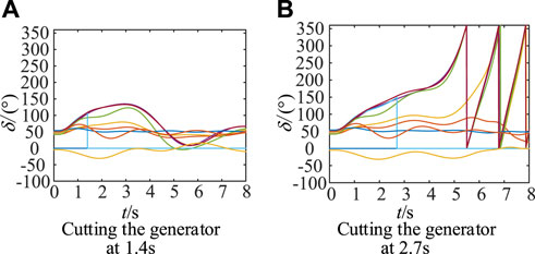
FIGURE 15. Transient response curve after emergency control measures.
The method proposed in this study incorporates the Savitzky-Golay filtering processing technique for MLE calculation, endowing it with a considerable degree of noise immunity. Typically, the signal noise ratio (SNR) of PMU measurements surpasses 100, ensuring that the measurement error remains below 1 percent (Dasgupta and Paramasivam, 2013). A Gaussian noise with a SNR of 60 dB is added to the above instability example to simulate the actual PMU measurement noise. The results of the MLE curves for both algorithms are shown in Figure 16.
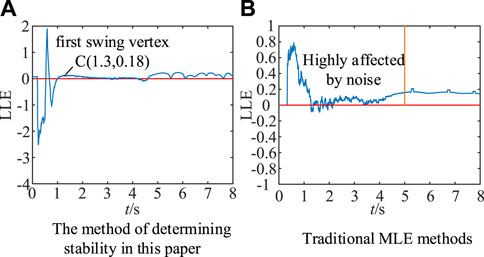
FIGURE 16. Result after adding Gaussian noise.
From Figure 16A, in the method proposed in this paper, the addition of noise does not have a delayed effect on the time point corresponding to when the MLE curve reaches the apex of the first swingback in the discriminant. There is no effect on the time required for the stability discrimination.
From Figure 16B, in the traditional MLE method, the MLE curve is affected by noise with a larger magnitude in the first 5 s, when it is not appropriate to discriminate the MLE sign. Until the 5 s curve is slightly smooth, then the MLE symbols can be discriminated, but the discriminatory timeliness is poor.
From this, the method proposed in this paper has strong anti-noise ability.
To further validate the reliability of the proposed method, a traversing fault test is performed at the 39-node system. So that all lines excluding the generator node have a three-phase short-circuit fault (N−1) at the moment of 0.2 s. The double return line defaults to disconnect the first return line. The fault removal moments are traversed sequentially from 0.2 to 3 s in steps of 0.2 s. Total 480 groups of faults.
In each set of tests, the key branch was quickly identified after fault removal using the method proposed in Section 4.3. The MLE curve of the sBTTC index of the key branch is analyzed to determine the system stability. Comparison is made with two judgments. These two criteria are the criterion based on the stability characteristic quantity (generator angle greater than 180°) and the criterion based on the traditional MLE calculation method. To increase the conservatism, the time window based on the traditional MLE calculation method is chosen as the end moment of the simulation. The third of these methods uses the batBPA batch program, and the first and second methods are implemented by building a Python interface to BPA. The statistical results are shown in the following table.
From Table 1, the method of this paper can successfully identify 404 sets of destabilizing samples through the traversal failure test. If based on the amount of stabilization features, the recognition rate of the destabilization samples of this paper’s criterion is 100%. The stabilization misjudgment rate is 2.6%. And in the test results, the average time required to judge the system stability is within 1.4 s after failure. The first method in the above table is obviously better than the second.
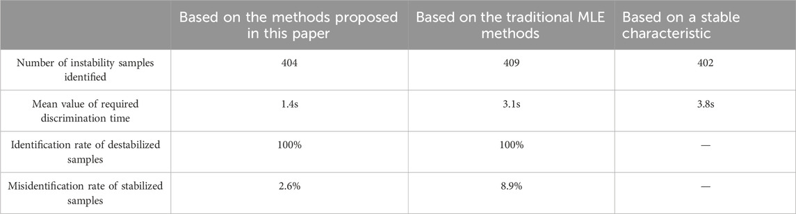
TABLE 1. Comparison table.
In a specific reference year, the local structure of the transmission grid in the eastern region of Inner Mongolia is illustrated in Figure 17. The eastern Mengdong grid is interconnected with the Northeast grid through three 500 KV AC branch circuits: Xinglong-Lingdong, Yifang-Fengtun, and Yimin-Hongcheng. Additionally, the eastern Mengdong grid features a ±500 KV/3000 MW UHVDC connection in Yimin-Mujia, forming a mixed pattern of AC and DC with the AC branch circuits.

FIGURE 17. DC hybrid grid.
During a particular operational scenario, the Yimin-Mujia UHVDC transmits 2000 MW, while the Xinglong-Lingdong, Yifang-Fengtun, and Yimin-Hongcheng three 500 KV AC branch circuits transmit 3520 MW. The Yifang-Fengtun line plays a crucial role in the structure of the Northeastern local grid. Unfortunately, it experiences a three-phase permanent short-circuited double circuit fault at 0.2 s, leading to the isolation of the faulty line and parallel line disturbances at 0.3 s. Generator angle curve and node voltage curve as shown in Figures 18A, B can be seen, by the short-circuit impact fault, electrical connection weakening, the tide of a wide range of transfer and other factors, the angle of the Mengdong group of machines relative to the main grid group of machines out of synchronisation, the node voltage of the system to occur a large drop and show the characteristics of the cyclic oscillations, the system occurred in the transient angle destabilisation.
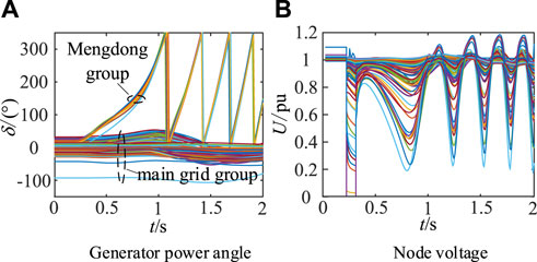
FIGURE 18. Transient response curve of DC hybrid system.
Concomitant with the aforementioned destabilisation process, the response curve of the sBTTC index for the 500 KV AC lines throughout the network is depicted in Figure 19A. Notably, the Yimin-Hongcheng branch consistently displays the smallest sBTTC index during the initial decline stage of the sBTTC index. Furthermore, the branch droop voltage coefficient ξv ∈ [1,2], as illustrated in Figure 19B, reaffirms the key nature of the Yimin-Hongcheng branch within the network.
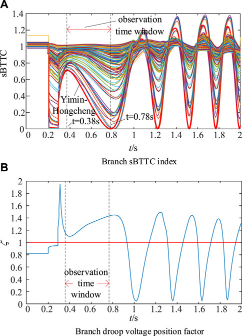
FIGURE 19. sBTTC index vs. dropout voltage position factor.
The MLE-t curve of sBTTC index of Emin-Hongcheng branch is shown in Figure 20A. Meanwhile, the MLE-t curve of the angle trajectory of the generator Ewenk, for example, is solved using the traditional method for the overrun unit Ewenk as shown in Figure 20B.
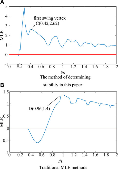
FIGURE 20. MLE-t curve under the destabilisation case.
From Figure 20A, at 0.42 s, the first pendulum fixed point value of MLE curve is 2.62, which is positive, and at this time, the sBTTC index is 0.67. To judge the instability of Mengdong grid, the maximum relative angle difference of the generator at this time is 1.48 rad.
From Figure 20B, under the premise of setting the observation time window appropriately, the MLE sign can be determined to be positive only at 0.96 s. It is only at this moment that the traditional MLE calculation method can determine the instability of the Mengdong power grid. Compared with the method in this paper, the timeliness of the determined 0.96 s is poor. Moreover, if the observation time window is not set properly, it is easy to misjudge that the system is stable at 0.5 s. Therefore, the proposed method is better than the one in this paper. Therefore, the method proposed in this paper has more advantages than the traditional MLE solving method.
Similarly, considering the communication delay, the implementation of emergency control measures at 0.5 s and the removal of the Ewenke unit can restore the stability of the system. At 1.0 s, resection of Ewenke unit cannot make the system restore stability.
In order to verify the effectiveness of this paper’s method in a large system, the Gaussian noise interference with SNR of 60 dB is added to the above example, and the results of the MLE curve calculated by the proposed method are shown in Figure 21A, and the results of the MLE curve calculated by the traditional method are shown in Figure 21B.
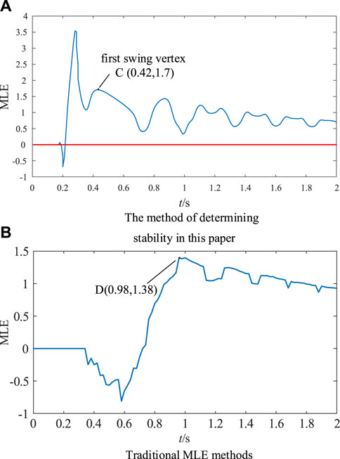
FIGURE 21. Result after adding Gaussian noise.
From Figure 21A, it can be seen that after adding 60 dB noise to the sampled data, the time point corresponding to the first pendulum vertex of the MLE curve obtained by the method in this paper is unchanged, and the judgement of the stability time before and after the addition of noise is 0.42 s, the judgement of the stability time is unchanged, and the curve is still smooth.
As can be seen from Figure 21B, after adding 60 dB noise to the sampled data, the judgement of stability time of the traditional method is 0.98 s, and the difference between before and after is not significant. However, the MLE curve fluctuates significantly after the addition of noise before the time node, which is not conducive to the identification of the MLE symbols, and it is very easy to lead to the occurrence of misjudgment.
The method proposed in this paper has strong noise immunity in large systems as well. And the example of Mengdong Power Grid shows that the method has better applicability in large-scale power systems. It can judge the system stability level in time and is not easily affected by noise.
After a system generator is destabilized, certain combinations of electrical quantities in the branches of the network contain information characterizing the system stability. In this paper, MLE analysis is carried out for the key branch response information, and the main conclusions of the study are as follows.
(1) Under both system stability and instability patterns, the sBTTC index trajectories in the critical branches show two typically different characteristics. The system transient stability problem can be transformed into a problem of MLE analysis of sBTTC index time series data.
(2) In this paper, the MLE stability discrimination principle is utilised to analyse the dynamic characteristics of the sBTTC exponential response trajectory. Combining the sBTTC method with the MLE method, the MLE transient stability analysis method based on the key branch response is proposed. Compared with the traditional method, the method has the following advantages: easy access to information sources, rapid discriminative stability, strong noise resistance, and strong engineering application value.
(3) On the one hand, the proposed method determines the optimal dynamic observation time window through the variation of the sBTTC index trajectories of the key branches. On the other hand, the stability discrimination is realised through the dynamic characteristics of MLE curves. The method still achieves transient power angle steady state assessment quickly and accurately under large-scale systems, and overcomes the difficulty of finding the optimal time window for MLE stability monitoring methods.
The original contributions presented in the study are included in the article/Supplementary Material, further inquiries can be directed to the corresponding author.
ZN: Writing–original draft. CZ: Writing–review and editing. SL: Writing–original draft. YS: Writing–review and editing. FN: Validation, Writing–review and editing.
The author(s) declare financial support was received for the research, authorship, and/or publication of this article. This work is supported by National Key Research and Development Program projects “Response-driven intelligent enhancement analysis and control of large grid stability Technology” (2021YFB2400800).
Authors ZN and CZ were employed by China Electric Power Research Institute Co., Ltd.
All claims expressed in this article are solely those of the authors and do not necessarily represent those of their affiliated organizations, or those of the publisher, the editors and the reviewers. Any product that may be evaluated in this article, or claim that may be made by its manufacturer, is not guaranteed or endorsed by the publisher.
Andersson, G., Donalek, P., Farmer, R., Hatziargyriou, N., Kamwa, I., Kundur, P., et al. (2005). Causes of the 2003 major grid blackouts in North America and Europe, and recommended means to improve system dynamic performance. IEEE Trans. Power Syst. 20 (4), 1922–1928. doi:10.1109/TPWRS.2005.857942
Chen, G., Li, M., Xu, T., Zhang, J. Y., and Wang, C. (2017). Practice and challenge of renewable energy development based on interconnected power grids[j]. Power Syst. Technol. 41 (10), 3095–3103. doi:10.7500/AEPS2017120004
Dasgupta, S., Paramasivam, M., Vaidya, U., and Ajara, V. (2015). PMU-based model-free approach for real-time rotor angle monitoring. IEEE Trans. Power Syst. 30 (5), 2818–2819. doi:10.1109/TPWRS.2014.2357212
Dasgupta, S., Paramasivam, M., Vaidya, U., and Ajjarapu, V. (2013). Real-time monitoring of short-term voltage stability using PMU data. IEEE Trans. Power Syst. 28 (4), 3702–3711. doi:10.1109/tpwrs.2013.2258946
Dasgupta, S., Paramasivam, M., Vaidya, U., and Ajjarapu, V. (2013). Real-time monitoring of short-term voltage stability using PMU data. IEEE Trans. Power Syst. 28 (4), 3702–3711. doi:10.1109/TPWRS.2013.2258946
Gou, J., Liu, J., Taylor, G., et al. (2015a). Fast assessment of power system transient stability based on generator pair transient potential energy sets. Grid Technol. 39 (02), 464–471. doi:10.13335/j.1000-3673.pst.2015.02.026
Gou, J., Liu, J. Y., Taylor, G., et al. (2015b). Rapid assessment of power system transient stability based on generator pair transient potential energy sets. Grid Technol. 39 (02), 464–471. doi:10.13335/j.1000-3673
Huang, D., Sun, H., Zhou, Q., Zhang, J., Jiang, Y. L., and Zhang, Y. C. (2020). Online monitoring of transient stability based on the dynamic characteristics of maximum Lyapunov exponent of response trajectory. Power Autom. Equip. 40 (4), 48–55. doi:10.16081/j.epae.202004002
Kundur, P., et al. (2004). Definition and classification of power system stability IEEE/CIGRE joint task force on stability terms and definitions. IEEE Trans. Power Syst. 19 (3), 1387–1401. doi:10.1109/TPWRS.2004.825981
Lin, Li, Wu, C. C., and Qi, J. (2016). Analysis of emergency cutover strategies under severe faults in large-scale wind-fire hybrid feeder systems. Power Grid Technol. 40 (3), 882–888. doi:10.13335/j.1000-3673.pst.2016.03.032
Liu, C. W., Thorp, J. S., Lu, J., Thomas, R., and Chiang, H-D. (1994). Detection of transiently chaotic swings in power systems using real-time phasor measurements. IEEE Trans. Power Syst. 9 (3), 1285–1292. doi:10.1109/59.336138
Liu, D. W., et al. (2013). Response-based online quantitative assessment method for transient stabilisation potential of power grids. Chin. J. Electr. Eng. 33 (4), 85–95+12. doi:10.13334/j.0258-8013.pcsee.2013.04.014
Liu, R., Chen, L., Min, Y., et al. (2018). A linear approximation method for the boundary of dynamic security domain of wind-fire bundled delivery system. Grid Technol. 42 (10), 3211–3218. doi:10.13335/j.1000-3673
Liu, T., Tang, Z., Huang, Y., Xu, L., and Yang, Y. (2023). Online prediction and control of post-fault transient stability based on PMU measurements and multi-task learning. Front. Energy Res. 10, 1084295. doi:10.3389/fenrg.2022.1084295
Mu, G., Wang, Z., Han, Y., et al. (1993). Quantitative analysis of transient stability-trajectory analysis method. Chin. J. Electr. Eng. (03), 25–32. doi:10.13334/j.0258-8013
Paudyal, S., Ramakrishna, G., and Sachdev, M. S. (2010). Application of equal area criterion conditions in the time domain for out-of-step protection. IEEE Power Transm. Lett. 25 (2), 600–609. doi:10.1109/tpwrd.2009.2032326
Qin, X., Bi, T., Yang, Q., et al. (2008). Power system transient stability assessment based on WAMS dynamic trajectories. Automation Electr. Power Syst. 32 (23), 18–22.
Ravikumar, G., and Khaparde, S. A. (2018). Taxonomy of PMU data based catastrophic indicators for power system stability assessment. IEEE Syst. J. 12 (1), 452–464. doi:10.1109/JSYST.2016.2548419
Shaopan, W., Yang, M., Han, X., et al. (2017). An online identification method of transient angle stability using the MLE index of machine terminal voltage amplitude trajectory. Chin. J. Electr. Eng. 37 (13), 3775–3786. doi:10.13334/j.0258-8013.pcsee.162476
Sun, H., Tang, Y., and Ma, S. (2006). A commentary on definition and classification of power system stability. Power Syst. Technol. 30 (17), 31–35. doi:10.13335/j.1000-3673.pst.2006.17.006
Tang, C. (2014). Response-based wide-area security and stability control of power systems. Chin. J. Electr. Eng. 34 (29), 5041–5050. doi:10.13334/j.0258-8013.pcsee.2014.29.005
Tian, X., Zhao, L., Tong, C., Meng, X., Bo, Q., Chen, Y., et al. (2023). Optimal configuration of grid-side energy storage considering static security of power system. Front. Energy Res. 1. doi:10.3389/frsgr.2022.1110871
Wadduwage, D. P., Wu, C. Q., and Anakie, U. D. (2013). Power system transient stability analysis via the concept of Lyapunov Exponents. Electr. Power Syst. Res. 104, 183–192. doi:10.1016/j.epsr.2013.06.011
Wang, M., Wu, J., et al. (1991). Large power grid system technology. Beijing, China: Water Conservancy and Electric Power Press, 140.
Xie, H., Zhang, B., Yu Guang, L., et al. (2006). Identification of power system transient stability based on phase trajectory concavity. Chin. J. Electr. Eng. 2006 (05), 38–42. doi:10.13334/j.0258-8013.pcsee.2006.05.007
Xue, F., and Xue, Y. (1999). Stability-preserving reduced dimensional mapping of multi-rigid body disturbed trajectories. Power Syst. Autom. 24, 11–15.
Xue, Y., Van Custom, T., and Ribbens-Pavella, M. (1989). Extended equal area criterion justifications, generalizations, applications. IEEE Trans. Power Syst. 4 (1), 44–52. doi:10.1109/59.32456
Yan, J., Liu, C.-C., and Vaidya, U. (2011). PMU-based monitoring of rotor angle dynamics. IEEE Trans. Power Syst. 26 (4), 2125–2133. doi:10.1109/TPWRS.2011.2111465
Zeng, Y., Chang, J., Qin, C., et al. (2018). A practical dynamic safety domain construction method based on phase trajectory analysis. Chin. J. Electr. Eng. 38 (07), 1905–1912. doi:10.13334/j.0258-8013
Zheng, C., Sun, H., and Deng, J. (2022). Active detrainment control of angle instability based on wide-area branch response. Chin. J. Electr. Eng. 42 (11), 3885–3896. doi:10.13334/j.0258-8013.pcsee.211592
Zheng, C., Sun, H., and Li, H. (2021a). Response-based transient transmission capacity index and emergency control of branch circuits. Chin. J. Electr. Eng. 41 (02), 581–592. doi:10.13334/j.0258-8013.pcsee.200969
Keywords: maximum Lyapunov exponent, transient branch transmission capacity index, transient angle stability, the key branch, wide-area measurement system
Citation: Niu Z, Zheng C, Lv S, Shan Y and Ni F (2024) Transient angle stability analysis of maximum Lyapunov exponent based on the key branch response information. Front. Energy Res. 11:1267303. doi: 10.3389/fenrg.2023.1267303
Received: 26 July 2023; Accepted: 19 December 2023;
Published: 23 January 2024.
Edited by:
Hao Xiao, Chinese Academy of Sciences (CAS), ChinaCopyright © 2024 Niu, Zheng, Lv, Shan and Ni. This is an open-access article distributed under the terms of the Creative Commons Attribution License (CC BY). The use, distribution or reproduction in other forums is permitted, provided the original author(s) and the copyright owner(s) are credited and that the original publication in this journal is cited, in accordance with accepted academic practice. No use, distribution or reproduction is permitted which does not comply with these terms.
*Correspondence: Zhenbo Niu, bml1emhlbmJvX2VwcmlAMTYzLmNvbQ==
Disclaimer: All claims expressed in this article are solely those of the authors and do not necessarily represent those of their affiliated organizations, or those of the publisher, the editors and the reviewers. Any product that may be evaluated in this article or claim that may be made by its manufacturer is not guaranteed or endorsed by the publisher.
Research integrity at Frontiers
Learn more about the work of our research integrity team to safeguard the quality of each article we publish.