Two-tier coordinated optimal scheduling of wind/PV/hydropower and storage systems based on generative adversarial network scene generation

In order to achieve the economic consumption of renewable energy in a multi-energy power system including wind/PV/hydropower and energy storage, a two-tier coordinated optimal scheduling method based on generative adversarial network (GAN) scenario generation is proposed in this paper. First, an upper-tier optimization model for the operation of the load and storage system is established to achieve the objective of minimizing the load fluctuation and the cost of energy storage plants. Furthermore, a lower-tier optimization model to minimize the system operation cost and tide risk is established for the optimization operation of renewable energy generation. Second, an improved generative adversarial network is proposed to generate the operation scenes for evaluating the uncertainty characteristics of the wind and photovoltaic (PV) generation. Then, an improved coati optimization algorithm (COA) is used to solve the proposed optimization problem. Finally, the IEEE 30-bus system is selected as the example system for verifying the proposed method. The simulation results corroborate the validity and feasibility of the proposed method.

1 Introduction

Limited fossil energy sources and global greenhouse gas issues have led to the increased interest in the utilization and development of renewable energy. The continued increase in renewable energy generation poses a risk to the safe and stable operation of new power systems. Due to the intermittent and fluctuating nature of renewable energy sources, connecting high-capacity wind and photovoltaic power generation into the power system will seriously affect the power quality and the stable operation of the grid (Sezer et al., 2019). The scheduling and operation of various power sources, including wind/PV/hydro/thermal and storage, are of increasing concern (An et al., 2020; Gejirifu et al., 2022). Based on this background, the synergistic operation of PV/wind energy with other renewable energy sources (e.g., hydropower or energy storage) is a current research hot spot. It can accommodate more PV and wind power generation without affecting the safety and reliability of the power system.

Research on coordinated and optimal scheduling of power systems is one of the current research hot spots, and many results have been achieved in this field by previous authors. For example, Xia et al. (2020) proposed a scheduling model based on wind/PV generation and load demand in which a mixed integer linear programming mode l is used to achieve economic operation of the system when considering the power regulation speed and capacity of the generation side. Based on the analysis of the stochastic and intermittent nature of wind power output and PV output, Zhang et al. (2021) considered dynamic frequency response constraints in the conventional optimal scheduling model. The objective function is to maximize the generation cost of the thermal generator and the storage value of the hydropower plant. Zhang et al. (2018) studied the short-term optimal operation of the wind power portfolio of the Yalong River multi-energy complementary clean energy base using the progress optimization algorithm (POA). To maximize the total generation capacity and minimize the energy production cost of the hybrid system, Hounnou et al. (2019) proposed a model of a run-of-river mini-hydropower plant hybrid generation system based on a non-dominated ranking genetic algorithm. Zhao et al. (2020) proposed a multi-energy optimal scheduling model of wind-nuclear-thermal-storage-gas, considering the consumption risk of nuclear and wind power.

Wang et al. (2022) investigated the optimal scheduling of an integrated power system considering long-term voltage stability constraints for wind energy grid connections. The operational constraints representing the integrated power and gas system are formulated using a second-order cone planning formulation. Hu et al. (2019) developed a unit model for wind power consumption in CHP systems by analyzing the topological differences between the power and thermal systems. The objective function is to minimize total coal consumption and environmental costs. To address the potential mismatch between renewable energy generation and load, an integrated optimal scheduling strategy model with interactions between generation and consumption was proposed by Liu et al. (2021). In order to achieve an economic strategy for wind abandonment and deep peaking, a unit optimization model was proposed by Yang et al. (2020). The model considered the cost of deep peaking and wind abandonment of thermal power units. Zhang and Wang (2018) proposed a hierarchical distributed coordination optimal scheduling strategy for active distribution networks. The strategy considered wind power uncertainty, and an iterative solution method based on cascaded analytical objectives was used.

The penetration of renewable energy in the power system is increasing in the context of carbon peaking and carbon-neutral strategies. Characterizing the inherent variability and uncertainty of renewable energy is critical. Accurate modeling of renewable energy uncertainties plays an important role in power system operation, planning, and decision-making. Scene generation is a key approach to providing system planners and operators with a range of possible power scenarios to make decisions in the future. Yang et al. (2021) proposed a coordinated interval optimization scheduling method considering the uncertainty of renewable energy. It describes the uncertainty of wind and PV power generation through interval numbers. Huang et al. (2022) proposed a typical scene generation method based on Latin hypercube sampling and spectral clustering. The method enables efficient typical scenario generation considering stochastic fluctuations in renewable energy output and load demand. In order to generate representative daily scenarios of wind power, a wind power time series scene generation method is proposed based on a longitudinal and horizontal clustering strategy with reference to Guan et al. (2018). Based on the affinity propagation clustering algorithm, discrete stochastic models are obtained by cluster analysis along the longitudinal and horizontal directions. Jithendranath and Das (2020) proposed a hybrid scenario and Monte Carlo approach to measure the uncertainty involved in the multiple energy demands of a microgrid, considering the correlation between electricity, heating, and cooling loads and wind and PV generation. This model helps in depicting the probability of renewable power uncertainty. Liang et al. (2019) used a probabilistic paradigm to construct mixing probabilities that describe the uncertainty of renewable energy sources. Jiang et al. (2018), Sadek et al. (2021), and Wang et al. (2021) used generative adversarial networks as a data-driven scene generation method.

In order to realize the economic consumption of renewable energy in a multi-energy power system, including wind power/PV/hydropower and energy storage, while ensuring the security and stability of the system currents, a two-tier coordinated optimal scheduling method based on an improved generative adversarial network scene is proposed.

The main contributions are summarized as follows:

1. This paper proposes a two-tier coordinated optimal scheduling strategy for power systems containing wind power/PV/hydropower and energy storage. It can reduce the load peak-to-valley difference and improve the space for renewable energy consumption. It can also ensure the safe and stable operation of the system.

2. A wind power and PV scene generation method based on the improved generative adversarial network is proposed for constructing typical scenarios of renewable energy generation. The improved GAN can weaken the randomness and uncertainty of renewable energy power generation.

3. Based on the coati optimization algorithm, five improvement strategies are fused with the coati optimization algorithm and the retrograde improvement to enhance its optimization-seeking capability.

The remainder of this paper is organized as follows: Section 2 describes the two-tier coordinated optimal scheduling model. In Section 3, the improved GAN-based scene generation methods for wind power and PV are presented. In Section 4, five improved strategies based on the coati optimization algorithm are proposed. In Section 5, the optimization model is solved and simulations are performed to validate it on the improved IEEE 30-bus system. Conclusion is reported in Section 6.

2 Two-tier coordinated optimal dispatch model for wind/PV/hydropower and energy storage systems

A two-tier coordinated optimal scheduling model based on energy interaction and grid operation is constructed from the perspectives of economy, security, and stability. The objective function of the upper-tier scheduling model is to minimize load fluctuation and the cost of the energy storage plant. It determines the load profile and the daytime charging and discharging strategy of the energy storage system and passes them to the lower-tier scheduling model. The objective function of the lower-tier scheduling model is to minimize system operation costs and tide risk and determine the optimal scheduling strategy for scenic water. After the feedback of the optimal strategies of each layer of the dispatch model, the optimization results that satisfy the overall optimal operation of the grid are calculated. The overall framework of the system is shown in Figure 1.

FIGURE 1

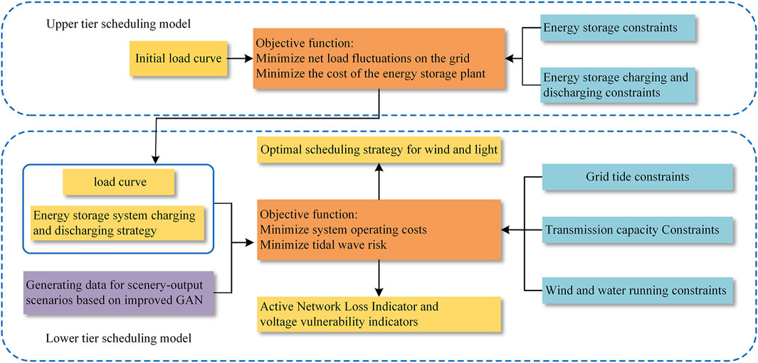
FIGURE 1. Framework diagram of the two-tier coordination scheduling model.

2.1 Upper-tier optimal scheduling model

The upper-tier scheduling model takes load fluctuation and minimization of energy storage plant cost as the objective function. It aims to achieve the objectives of reducing the fluctuation of the grid and improving the consumption capacity of wind and PV by using energy storage plants.

2.1.1 Objective function

1. Load fluctuation

The load volatility indicator can reflect stability and fluctuation within 1 day after load optimization. The mathematical formulas are as follows:

$\min F_1=\frac{{\displaystyle \sum _{t=1}^{23}}\left|P_{net}\left(t+1\right)-P_{net}\left(t\right)\right|}{{\displaystyle \sum _{t=1}^{24}}{P}_{net}\left(t\right)}\cdot {\epsilon }_{net},(1)$

$P_{net}\left(t\right)=P_{load}\left(t\right)+{\displaystyle \sum _{m=1}^{N_M}}{\eta }_c{P}_{S,t}^c\left(t\right)-{\displaystyle \sum _{m=1}^{N_M}}{\eta }_d{P}_{S,t}^d\left(t\right),(2)$

where $F_1$ and ${\epsilon }_{net}$ are the penalty cost and penalty coefficient for load fluctuation, respectively; $P_{net}\left(t+1\right)$ is the load value at time $\left(t+1\right)$; $P_{net}\left(t\right)$ is the load value at time $t$; $P_{S,t}^c$ is the charging power of the energy storage plant at time $t$; $P_{S,t}^d$ is the discharging power of the energy storage plant at time $t$; ${\eta }_c$and ${\eta }_d$ are the charging and discharging efficiency of the energy storage plant, respectively; and $N_M$ is the total number of energy storage plants.

2. Energy storage plant costs

During the operation of the energy storage plant, the cost of the energy storage plant consists of two parts, namely, operation and maintenance costs and grid-connected environmental benefits, which are expressed as follows:

$\begin{array}{l}\min F_2=f_{sc}-f_{ss}={\displaystyle \sum _{t=1}^T}{\beta }_{soc}({\eta }_d{P}_{St}^d+{\eta }_c{P}_{St}^c)-\\ {\displaystyle \sum _{t=1}^T}\left({\gamma }_{soc}{\eta }_d{P}_{dis,t}\right),\end{array}(3)$

where $f_{sc}$ is the operation and maintenance cost of the energy storage plant, $f_{ss}$ is the environmental benefit of the energy storage plant, ${\beta }_{soc}$ is the operating cost coefficient of the energy storage plant, ${\gamma }_{soc}$ is the environmental benefit coefficient generated by the grid-connected energy storage plant, and the meanings of the remaining variables are consistent with the previous paper.

2.1.2 Constraint

$\left\{\begin{array}{l}{S}_{\min }\le S_{st}\le S_{\max },\\ u_t^c{P}_{S\min }^c\le P_{St}^c\le u_t^c{P}_{S\max }^c,\\ u_t^d{P}_{S\min }^d\le P_{St}^d\le u_t^d{P}_{S\max }^d,\end{array}\right.(4)$

where $S_{st}$ is the charge state of the energy storage plant at time $t$; $S_{\mathit{max}}$ and $S_{\mathit{min}}$ are the upper and lower limits of the charge state of the energy storage plant, respectively; $u_t^c$ and $u_t^d$ are the charge and discharge states of the energy storage plant, respectively; $P_{S\max }^c$ and $P_{S\min }^c$ are the maximum and minimum values of the charge power, respectively; and $P_{S\max }^d$ and $P_{S\min }^d$ are the maximum and minimum values of the discharge power, respectively.

2.2 Lower-tier optimal scheduling model

The lower-tier scheduling model aims to minimize system operation costs and tide risk. The upper tier transmits the load profile and the results of the energy storage system charging and discharging strategy to the lower tier, and after calculation, the best scheduling strategy for wind farms, PV plants, and hydropower units can be obtained, and the process satisfies the system tide constraint. It ensures the safe and stable operation of the grid.

2.2.1 Objective function

In the lower model, the economic indicators include the operation and maintenance costs of wind farms, PV plants, and hydropower units; the start-up and shutdown costs of hydropower units; the environmental benefits of grid connection and consumption of wind farms, PV plants, and energy storage systems; and the cost of power purchase and sale of the system.

$\left\{\begin{array}{l}\min F_3=f_1+f_2-f_3+f_4,\\ f_1={\displaystyle \sum _{t=1}^T}\left({\mu }_w{P}_{w,t}^{acc}+{\mu }_{pv}{P}_{pv,t}^{acc}+{\mu }_{hy}{P}_{hy,t}^{acc}\right),\\ f_2={\displaystyle \sum _{t=1}^T}{\displaystyle \sum _{j=1}^{N_G}}{s}_{j,t}{u}_{j,t}\left(1-u_{j,t-1}\right),\\ f_3={\displaystyle \sum _{t=1}^T}\left({\beta }_w{P}_{pw,t}^{acc}+{\beta }_{pv}{P}_{pv,t}^{acc}\right),\\ f_4={\displaystyle \sum _{t=1}^T}\left({\rho }_{PC}^b\left(t\right)P_{line}\left(t\right)\Delta t-{\rho }_{PC}^s\left(t\right)P_{line}\left(t\right)\Delta t\right),\end{array}\right.(5)$

where $F_3$ is the system economic index; $f_1$ is the system operation and maintenance cost; ${\mu }_w$, ${\mu }_{pv}$, and ${\mu }_{hy}$ are the operating cost coefficients of wind power, PV, and hydropower units, respectively; and $P_{w,t}^{acc}$, $P_{pv,t}^{acc}$, and $P_{hy,t}^{acc}$ are the power consumption of wind power, PV, and hydropower units at time $t$, respectively. $f_2$ is the start–stop cost of hydropower unit j; $s_{j,t}$ is the start–stop cost of hydropower unit $j$ at time $t$; $u_{j,t}$ is the start–stop state of hydropower unit $j$ at time $t$; and $f_3$ is the environmental benefit of wind power, PV, and energy storage consumption. ${\beta }_w$ and ${\beta }_{pv}$ are the environmental benefit coefficients for grid-connected consumption of wind power and PV, respectively; $f_4$ is the cost of power purchase and sale; ${\rho }_{PC}^b\left(t\right)$ and ${\rho }_{PC}^s\left(t\right)$ are the unit price of power purchase and unit price of power sale to the superior grid at time $t$, respectively; $P_{line}\left(t\right)$ is the value of exchange power of the contact line at time $t$; and $\Delta t$ is the interval between the two time sampling.

Tidal risk indicators include the system active network loss rate and voltage vulnerability, and the active network loss rate of the grid is given as the percentage of the grid power loss to feed-in tariff. The grid vulnerability indicator is a state vulnerability indicator that starts with the operational security of the grid. It measures the risk resistance of the grid by analyzing the degree of voltage deviation from standard values at each bus to improve power quality. The higher the vulnerability, the more unstable the voltage at that bus is, and the lower the quality of power supplied, the less the risk-resistance is. The expressions are as follows:

$\left\{\begin{array}{l}\min F_4=f_{P\_loss}+f_{vol},\\ f_{P\_loss}=\frac{{\displaystyle \sum _{t=1}^T}{\displaystyle \sum _{i,j\in M_L}}\left[G_{ij}\left(U_{i,t}^2+U_{j,t}^2-2U_{i,t}{U}_{j,t}\cos {\delta }_{ij,t}\right)\right]}{{\displaystyle \sum _{t=1}^T}\left(P_{w,t}^{acc}+P_{pv,t}^{acc}+P_{hy,t}^{acc}+P_{S,t}^d\right)},\\ f_{vol}=\frac{1}{24}{\displaystyle \sum _{t=1}^{24}}\left(\frac{1}{2}BV\left(t\right)+\frac{1}{2}J\left(t\right)\right),\\ BV\left(t\right)=\frac{1}{N}{\displaystyle \sum _{i=1}^N}V\left(t,i\right),\\ V\left(t,i\right)=\frac{v\left(t,i\right)-v\left(t,i_{\min }\right)}{v\left(t,i_{\max }\right)-v\left(t,i_{\min }\right)},\\ v\left(t,i\right)=\frac{\left|\frac{U_{t,i}}{U_{i,o}}-1\right|}{0.07},\\ J\left(t\right)=1-{\left[\frac{{\displaystyle \sum _{i=1}^N}{p}_{t,i}{\mathit{log}}_2\left(\frac{1}{p_{t,i}}\right)}{{\mathit{log}}_{2}N}\right]}^{2\pi },\\ p_{t,i}=\frac{V\left(t,i\right)}{{\displaystyle \sum _{i=1}^N}V\left(t,i\right)},\end{array}\right.(6)$

where $F_4$ is the tidal risk indicator; $f_{P\_loss}$ is the active network loss rate of the system; $f_{vol}$ is the grid vulnerability; $M_L$ is all branches of the network; $G_{ij}$ is the set of conductances of buses $i$ and j; $U_{i,t}$ and $U_{j,t}$ are the voltages of buses $i$ and $j$ at time $t$, respectively; ${\delta }_{ij,t}$ is the phase angle difference between buses $i$ and $j$ at the beginning and end of the branch at time $t$; $BV\left(t\right)$ is the average vulnerability of the grid at time $t$; and $N$ is the total number of system buses. $v\left(t,i\right)$ is the vulnerability of any bus $i$ in the network at time $t$, and 0.07 is defined as the maximum voltage offset; $v\left(t,i_{\max }\right)$ and $v\left(t,i_{\min }\right)$, respectively, are the maximum and minimum vulnerability values of all buses at time $t$ before normalization. $V\left(t,i\right)$ is the normalized value of the vulnerability of each bus in time section $t$. $J\left(t\right)$ is the vulnerability balance of the network at time $t$, ranging from 0 to 1, with 0 representing absolute balance and 1 representing absolute imbalance, and $p_{t,i}$ is the ratio of the vulnerability of bus $i$ to the total vulnerability of the network at the current time.

2.2.2 Constraint

1. Grid tide constraints

$\left\{\begin{array}{c}{P}_i=U_i{\displaystyle \sum _{j\in i}}{U}_j\left(G_{ij}\cos {\theta }_{ij}+B_{ij}\sin {\theta }_{ij}\right),\\ Q_i=U_i{\displaystyle \sum _{j\in i}}{U}_j\left(G_{ij}\sin {\theta }_{ij}-B_{ij}\cos {\theta }_{ij}\right),\end{array}\right.(7)$

where $P_i$ and $Q_i$ are the injected active and reactive power at bus $i$, respectively; $U_i$ and $U_j$ are the voltage amplitudes at buses $i$ and $j$, respectively; $G_{ij}$ and $B_{ij}$ are the line conductance values between buses $i$ and $j$, respectively; and ${\theta }_{ij}$ is the voltage phase difference between buses $i$ and $j$.

2. Hydropower output constraint

$0<P_{h,t}^{hydro}\le P_{h,t,\max }^{hydro},(8)$

where $P_{h,t,\max }^{hydro}$ is the maximum output of the hydropower unit at moment $t$.

3. Minimum start–stop time constraints

$\left\{\begin{array}{l}{\displaystyle \sum _{k=t}^{t+T_{on}-1}}{u}_{gik}\ge T_{on}\left[u_{git}-u_{gi\left(t-1\right)}\right],\\ {\displaystyle \sum _{k=t}^{t+T_{on}-1}}\left(1-u_{gik}\right)\ge T_{off}\left[u_{gi\left(t-1\right)}-u_{git}\right],\end{array}\right.(9)$

where $T_{on}$ and $T_{off}$ are the maximum continuous start-up time and maximum continuous shutdown time of hydropower unit $i$, respectively.

4. Wind farm capacity constraint

$0<P_{W,t}^{wind}\le P_{W,t,\max }^{wind},(10)$

where $P_{W,t,\max }^{wind}$ is the maximum output of the wind farm at time $t$.

5. PV power plant output constraint

$0<P_{m,t}^{PV}\le P_{m,t,\max }^{PV},(11)$

where $P_{m,t,\max }^{PV}$ is the maximum power output of the PV plant at time $t$.

6. Line transmission capacity constraint

$0\le P_{Lt}\le P_{L\max },(12)$

where $P_{Lt}$ is the transmission power of line L at time $t$ and $P_{Lmax}$ is the maximum transmission capacity of line L.

3 Wind power and PV operation scene generation based on improved GAN

3.1 Generative adversarial network

A generative adversarial network is a deep learning model first proposed by Goodfellow in 2014. It uses deep neural networks to characterize non-linear relationships and exploit the intrinsic features of signal data by classifying complex signals. GAN consists of two parts: a generator and a discriminator. The core idea of GAN training is to establish the min–max game between the generator and discriminator. In the training phase of the neural network, the generator generates new samples by updating its own parameters, and the discriminator is used to judge the authenticity of the new samples generated by the generator. The objective function of GAN is as follows:

$\underset{G}{\min }\underset{D}{\max }V\left(G,D\right)=E_{x\sim P_x}\left[D\left(x\right)\right]-E_{z\sim P_z}\left[D\left(G\left(z\right)\right)\right],(13)$

where $E$ is the expected value of the corresponding distribution, $D\left(\sim \right)$ is the discriminator mapping function, $G\left(\sim \right)$ is the generator mapping function, $x$ is the generated sample data, $P_x$ is the generated sample data distribution, $z$ is the noisy sample data, and $P_z$ is the noisy sample data distribution.

GAN will provide a generator that accurately reflects the characteristics of the real sample distribution when the game between the generator and discriminator reaches the Nash equilibrium. In addition, the sample data generated by the generator are close to the real data and achieve scene substitution.

3.2 Improving the GAN model

3.2.1 GAN architecture construction

To improve the training stability of the original GAN model and the quality of the generated sample data, the paper uses a deep convolutional generative adversarial network (DCGAN) to construct the model. DCGAN uses the strong feature extraction ability of a convolutional neural network (CNN) to improve the quality of the generated sample data of the original GAN model. Compared with the original GAN model, the structure of DCGAN removes the fully connected layer and all pooling layers in the network and uses stepwise convolution instead of the pooling layers of the original GAN model.

1. Generator network structure

It contains four neural network layers, and each network layer contains a deconvolution layer, a batch normalization layer, and an activation function. The deconvolution layer changes the input dimension by using multiple deconvolution kernels. Each layer uses ReLU as the activation function, and the last layer uses tanh as the activation function.

2. Discriminator network structure

The sample changes its dimension after passing through the convolutional layers, and finally, the discriminator’s score for that sample is output through a fully connected layer with output dimension 1. All layers use LeakyReLU as the activation function. The structure of the discriminator designed in this paper is shown in Figure 2.

FIGURE 2

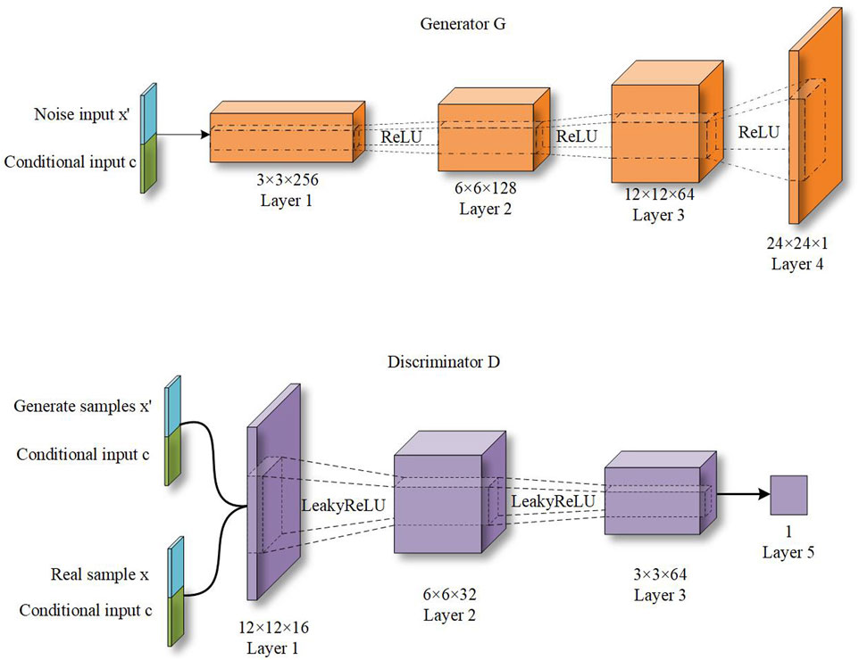
FIGURE 2. Generator and discriminator network depth structures.

3.2.2 GAN optimization design

1. Wasserstein GAN-gradient penalty (WGAN-GP)

The Jensen–Shannon divergence is used in original GAN to measure the similarity of two probability distributions, but during the training process, there may be cases where the scatter value is constant or meaningless, which leads to the disappearance of the gradient. To solve the problem of unstable GAN training, WGAN uses the Wasserstein distance to construct the model instead of the discriminator loss function in the original GAN model. The advantage is that when there is no overlap between two probability distributions, the distance between them can still be effectively described, and the Wasserstein distance can be defined as follows:

$W\left(P\left(x\right),P\left(x\prime \right)\right)=\frac{1}{K}\underset{{‖f‖}_L\le K}{\sup }{E}_{x\sim P\left(x\right)}\left(f\left(x\right)\right)-E_{x\prime \sim P\left(x\prime \right)}\left(f\left(x\prime \right)\right),(14)$

where $\mathit{sup}$ is the minimum upper bound, $x$ is the real sample data, $x^{\prime }$ is the generated sample data, $f$ is the discriminator using parameters for neural network fitting, $K$ is the Lipschitz constant for the discriminator $f$, and ${‖f‖}_L\le K$ is the K-Lipschitz limit satisfied by $f$.

However, WGAN enforces the Lipschitz continuity condition for weight cropping, which will reduce the training speed and learning efficiency. In order to avoid the WGAN gradient binarization, gradient disappearance, and explosion problems and further enhance the gradient controllability, this paper adds the gradient penalty term to the WGAN loss function to construct WGAN-GP to improve the model training efficiency. The objective function of WGAN-GP is as follows:

$\begin{array}{l}\underset{G}{\min }\underset{D}{\max }V\left(G,D\right)=E_{x\sim P_x}\left[D\left(x\right)\right]-E_{z\sim P_z}\left[D\left(G\left(z\right)\right)\right]\\ +\lambda E_{\widehat{x}\sim P\left(\widehat{x}\right)}\left[{\left({‖{\nabla }_{\widehat{x}}D\left(\widehat{x}\right)‖}_2-1\right)}^2\right],\end{array}(15)$

where $\lambda$ is the gradient penalty term coefficient; $\nabla$ is the gradient operator; $\widehat{x}$ is the random interpolation between the real and generated samples, $\widehat{x}=\xi x+\left(1-\xi \right)G\left(z\right)$; $\xi$ is the uniform distribution obeying [0,1]; $P\left(\widehat{x}\right)$ is the linear uniform sampling between the real and generated sample sampling points; and ${‖\cdot ‖}_p$ is the $p$-parameter.

2. Conditional GAN (CGAN)

GAN is trained by adding additional labels to the inputs of generators and discriminators. The problem of the unclear and uncontrollable direction of the original GAN generation is solved. The CGAN model is shown in Figure 3. Compared with the original GAN model, CGAN combines noise and additional conditions as inputs on the input side. The additional conditions can be any type of auxiliary information, such as category labels, or other modal data. The objective function of CGAN is as follows:

$\underset{G}{\min }\underset{D}{\max }V\left(D,G\right)=E_{x\sim P_x}\left[D\left(x|c\right)\right]-E_{z\sim P\left(z\right)}\left[D\left(G\left(z|c\right)\right)\right],(16)$

where $c$ is the label of the sample data.

3) Model evaluation metrics

FIGURE 3

FIGURE 3. CGAN model.

To verify the validity of the model, the average generation effect of the wind and PV scenes was evaluated using the root mean square error (RMSE) and the mean absolute error (MAE). The expressions for RMSE and MAE, respectively, are as follows:

$R_{MSE}=\sqrt{\frac{1}{N}{\displaystyle \sum _{n=1}^N}{\left(x_n^{\prime }-x_n\right)}^2,}(17)$

$M_{AE}=\frac{1}{N}\left|x_n^{\prime }-x_n\right|,(18)$

where $R_{MSE}$ and $M_{AE}$ are used to measure the error size between the generated samples and the real sample data, respectively (the smaller the value, the higher the accuracy of the generated sample data); $N$ is the total number of scenes generated; and $x_n$ and $x_n^{\prime }$ are the real samples and the data points corresponding to the generated samples, respectively.

3.3 Wind power and PV scene generation based on the improved GAN model

DCGAN uses convolutional layer feature extraction to explore the deep dynamic information of sample data to improve wind power and PV scene generation. WGAN-GP improves the training stability of wind power and PV scene generation models. CGAN mines the data feature association relationship between additional condition labels and wind power PV samples to enhance the interpretability of wind power and PV scene generation sample data.

In this paper, we combine the advantages of WGAN-GP, CGAN, and DCGAN as generator and discriminator network structures to construct a deep GAN model. It is applied to typical scene generation. The objective function of the improved GAN model is as follows:

$\begin{array}{l}\underset{G}{\min }\underset{D}{\max }V\left(G,D\right)=E_{x\sim P_x}\left[D\left(x|c\right)\right]-E_{z\sim P_z}\left[D\left(G\left(z|c\right)\right)\right]\\ +\lambda E_{\widehat{x}\sim P\left(\widehat{x}\right)}\left[{\left({‖{\nabla }_{\widehat{x}}D\left(\widehat{x}|c\right)‖}_2-1\right)}^2\right].\end{array}(19)$

The training steps of the improved GAN-based wind and PV power generation models are shown in Table 1. The specific process is as follows.

TABLE 1

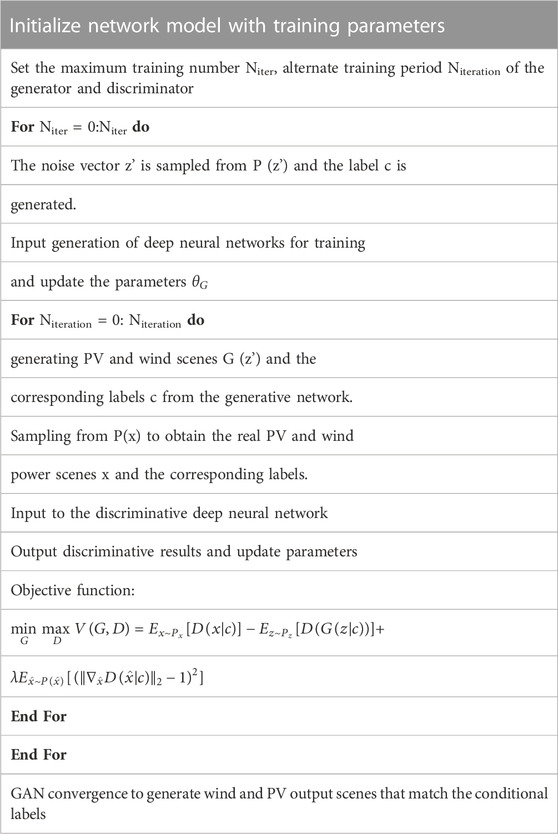
TABLE 1. Model training steps based on improved GAN.

Step 1. Initialize the model. Initialize the network model and training parameters. Normalize the training samples and obtain the random noise vector $z$ from the noise, obeying the standard normal distribution. Splice the noise with the conditional label $c$, and input the spliced data into the generator.

Step 2. Splice data. Longitudinally splice the conditional label $c$ with the sample data generated in Step 1. Input the result into the discriminator, and similarly, splice the conditional label $c$ with the wind power and PV real sample data. The results are fed into the discriminator.

Step 3. Train the discriminator network model. Fix the generator parameters, train the model of the discriminative network, feed the output and bias of the discriminator back to the discriminative network, and update the parameter ${\theta }_d$ by means of feed-forward propagation.

Step 4. Train the generative network model. Fix the discriminator parameters, and update the generator parameters ${\theta }_G$ by feedback.

Step 5. Model iterative training. The network model iterates through Steps 3 and 4 in a loop with Eq. 19 as the training objective, updating and correcting the parameters of the internal structure of the improved GAN model until the Nash equilibrium is reached, at which point the training stops.

Step 6. Save the results of the generated data. After the training, save the network structure and parameters of the generator and discriminator. Splice the conditional label c with noise in the test set and input it into the generator. The sample data of wind power and PV new energy output under this condition can be generated.

4 Two-tier optimal scheduling strategy and solution method

4.1 Scheduling strategy

In this paper, a two-tier coordinated optimal dispatch model of the system containing wind power/PV/hydropower and energy storage is developed. The optimization objectives include minimum load fluctuation and energy storage plant operation costs, minimum system operation costs, and minimum tidal current risk. Since multi-energy coordinated optimal scheduling involves more variables and constraints, the two-tier optimal scheduling model can simplify the computational complexity. It can also make full use of the peak-shaving and valley-filling characteristics of energy storage power plants while improving the consumption capacity of wind power and PV. The scheme makes decisions on the charging and discharging power of energy storage plants and optimizes the output of new energy generation by coordinating the upper and lower tiers and solving the problem in alternate iterations.

The upper-tier dispatch model uses the fast throughput capability of the energy storage system to track load fluctuations. The objective is to minimize the load fluctuation and the operating cost of the energy storage plant. By optimizing the output of the energy storage plant, the pressure on the hydropower units to cut the remaining load is reduced. It can make the output of wind/PV/hydropower and energy storage systems track the load profile optimally.

The upper and lower scheduling models are solved using the improved coati optimization algorithm. The upper tier is solved to obtain the load profile and the optimized charging and discharging strategy of energy storage plants. The lower tier is based on the load profile transferred from the upper tier, and the objective is to minimize the system operating cost and tidal risk. The final solution yields the optimal consumption strategy for wind power and PV, as well as the capacity plan for hydropower units, to determine the final optimal scheduling strategy.

4.2 Solution method based on the improved coati optimization algorithm

Coati optimization algorithm is a meta-heuristic algorithm proposed by Mohammad Dehghani et al. (2022) to simulate the behavior of coatis hunting to attack iguanas and escape from predators. It is difficult to obtain the global optimal solution when the “premature” phenomenon occurs. To address the shortcomings of COA, this paper adopts improvement strategies at different phases of the algorithm to enhance the global convergence ability of the algorithm.

4.2.1 Population initialization stage

During the population initialization process, the positions of coatis are randomly generated, and the update of individual positions depends on the update of population positions. To expand the effective search space of the algorithm and reduce the search blind spots, a refractive backward learning strategy is used to perturb the population positions. The idea of the refraction inverse learning strategy is derived from convex lens imaging. It extends the search range and enhances the search capability by generating a reverse position from the current coordinates, and its principle is shown in Figure 4.

FIGURE 4

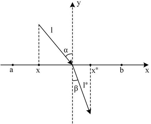
FIGURE 4. Refractive backward learning mechanism.

From the geometric relationship of the line segments in Figure 4, it can be inferred that

$\left\{\begin{array}{l}\sin \alpha =\frac{\left(\frac{\left(a+b\right)}{2}-x\right)}{l},\\ \sin \beta =\left(x^{*}-\left(a+b\right)/2\right)/l^{*},\\ n=\mathit{sin}\alpha /\mathit{sin}\beta ,\\ k=l/l*,\\ kn=\frac{\left(\left(a+b\right)/2-x\right)}{\left(x^{*}-\left(a+b\right)/2\right)},\end{array}\right.(20)$

where $\left[a,b\right]$ is the search interval of the solution on the $x$-axis; $l$ and $l*$ are the lengths of the incident and refracted rays, respectively; and $\alpha$ and $\beta$ are the angles of incidence and refraction, respectively.

The population location initialization formula for the fusion refraction backward learning strategy is as follows:

$\left\{\begin{array}{l}{x}_i\left(j\right)=l{b}_j+r\cdot \left(u{b}_j-l{b}_j\right),\\ x_i^{*}\left(j\right)=\frac{a_j+b_j}{2}+\frac{a_j+b_j}{2k}-\frac{x_i\left(j\right)}{k},\end{array}\right.(21)$

where $x_i\left(j\right)$ is the position of the ith coati in the jth dimension; $l{b}_j$ and $u{b}_j$ are the lower and upper bounds of the decision variables in dimension $i$, respectively; $x_i^{*}\left(j\right)$ is the refractive inverse solution of $x_i\left(j\right)$; $a_j$ and $b_j$ are the minimum and maximum values in dimension $j$ on the search space, respectively; and $r$ is a random number obeying uniform distribution in the interval $\left[\mathrm{0,1}\right]$.

4.2.2 Hunting and attack strategies

The COA population location update strategy was based on the coati attacking iguana behavior in Phase I. During this phase, the coati population was assumed to be divided into two parts: one-half of the coatis climbed trees to attack iguanas, and the other waited under the trees for iguanas to fall and preyed on them.

In this paper, we consider the integration of the Levy flight strategy for its location update to improve the local development of tree-climbing coatis. Levy flight is a special type of random wandering process. This form of wandering presents a combination of short-distance exploration and long-distance walking. The location update formula of the improved tree-climbing coatis is as follows:

$\begin{array}{l}{x}_i^{t+1}\left(j\right)=x_i^t\left(j\right)\cdot \left(u/\left({\left|v\right|}^{1/\beta }\right)\right)\\ +r\cdot \left(x_{bset}^t\left(j\right)-I\cdot x_i^t\left(j\right)\right),\end{array}(22)$

${\sigma }_u={\left(\frac{\mathrm{\Gamma }\left(1+\beta \right)\sin \frac{\pi \beta }{2}}{\mathrm{\Gamma }\left(\frac{1+\beta }{2}\right)\cdot \beta \cdot 2^{\left(\beta -1\right)/2}}\right)}^{1/\beta },(23)$

where $i=\mathrm{1,2},\dots ,\frac{N}{2}$, $N$ is the population size, $x_i^t\left(j\right)$ is the jth dimensional position of the ith coati at the current iteration number, $x_{best}^t$ is the best individual position in the current population, $I$ is a random integer in the set $\left\{\mathrm{1,2}\right\}$, $t$ is the current iteration number, and $\beta$ is a constant, generally set to 1.5, $u\sim N\left(0,{\sigma }_u^2\right)$, $v\sim N\left(\mathrm{0,1}\right)$.

In this paper, a sine–cosine optimization strategy is used to improve the position update of ground coatis and balance the global search and local exploration abilities of COA. It is based on the principle of gradually finding the optimal solution by using the fluctuation properties of the sine and cosine functions. The improved ground coati’s position update equation is as follows:

$I{g}_j^t=l{b}_j+r\cdot \left(u{b}_j-l{b}_j\right),(24)$

$x_i^{t+1}\left(j\right)=\left\{\begin{array}{l}{x}_i^t\left(j\right)+r_1\cdot \sin \left(r_2\right)\cdot \left|\left(r_{3}I{g}^t\left(j\right)-I\cdot x_i^t\left(j\right)\right)\right|,r_4<0.5,\\ x_i^t\left(j\right)+r_1\cdot \cos \left(r_2\right)\cdot \left|\left(r_{3}I{g}^t\left(j\right)-x_i^t\left(j\right)\right)\right|,r_4\ge 0.5,\end{array}\right.(25)$

$r_1=a-t\times \frac{a}{T},(26)$

where $i=\frac{N}{2}+1,\frac{N}{2}+2,\dots ,N$; $I{g}^t\left(j\right)$ is the current optimal individual; $T$ is the maximum number of iterations; $a$ is a constant, $a=2$; $r_2$ and $r_3$ are random numbers obeying uniform distribution in the interval $\left[\mathrm{0,2}\pi \right]$ and $\left[-\mathrm{2,2}\right]$, respectively; and $r_4$ is the selection control factor of the sine and cosine functions, which is the random number in the interval $\left[\mathrm{0,1}\right]$.

The optimal solution is updated using Eq. 27 after the first phase of COA.

$x_i^{t+1}\left(j\right)=\left\{\begin{array}{ll}{x}_i^{t+1}\left(j\right),& F\left(x_i^{t+1}\left(j\right)\right)<F\left(x_i^t\left(j\right)\right),\\ x_i^t\left(j\right),& else,\end{array}\right.(27)$

where $F$ is the fitness function.

4.2.3 Escape predator strategy

The COA population location update strategy is based on the coati fleeing predator behavior in Phase II. By simulating the predator avoidance strategy, each coati is made to generate a new location randomly near its current location. A spiral search strategy is introduced to avoid COA from falling into a local optimal solution at this phase, and the mathematical formulas are as follows:

$\left\{\begin{array}{c}l{b}_j^{local}=\frac{l{b}_j}{t},\\ u{b}_j^{local}=\frac{u{b}_j}{t},\end{array}\right.(28)$

$\begin{array}{l}{x}_i^{t+1}\left(j\right)=x_i^t\left(j\right)+D\cdot e^{bl}\cos \left(2\pi l\right)\\ +\left(1-2r\right)\cdot \left(l{b}_j^{local}+r\cdot \left(u{b}_j^{local}-l{b}_j^{local}\right)\right),\end{array}(29)$

$D=\left|2\cdot r\cdot x_{best}^t\left(j\right)-x_i^t\left(j\right)\right|,(30)$

where $u{b}_j^{local}$ and $l{b}_j^{local}$ are the upper and lower bounds of the jth dimensional decision variables updated with the number of iterations, respectively; $D$ is the distance between the optimal individual and the current individual; and $b$ defines the spiral shape, $l\in \left[-\mathrm{1,1}\right]$.

Furthermore, the t-distribution variation mechanism is used to perturb the individual positions of coatis to improve the COA finding ability. The t-distribution variational operator combines the Gaussian and Cauchy operators to replace the degree of freedom parameter of the t-distribution with the number of iterations of the algorithm. The t-distribution converges to the Cauchy distribution at the beginning of the algorithm iterations to improve the COA global search capability. As the number of iterations increases, the t-distribution converges to a Gaussian distribution to improve the COA local search level.

The iterative process of t-distribution variation is as follows:

$x_{i,new}^t\left(j\right)=x_{best}^t\left(j\right)+x_{best}^t\left(j\right)\cdot t\left(iter\right),(31)$

where $x_{i,new}^t\left(j\right)$ is the new position of the coati after the perturbation of the t-distribution variation, $x_{best}^t\left(j\right)$ is the current optimal individual position of the long-nosed raccoon, and $t\left(iter\right)$ is the t-distribution with the number of algorithm iterations $iter$ as the degrees of freedom.

The perturbation is updated using Eq. 32 after the perturbation:

$x_i^{t+1}\left(j\right)=\left\{\begin{array}{cc}{x}_{i,new}^t\left(j\right),& F\left(x_i^{t+1}\left(j\right)\right)<F\left(x_i^t\left(j\right)\right),\\ x_i^{t+1}\left(j\right),& else.\end{array}\right.(32)$

The solution flow of the improved COA-based two-tier coordinated optimal scheduling model is shown in Figure 5.

FIGURE 5

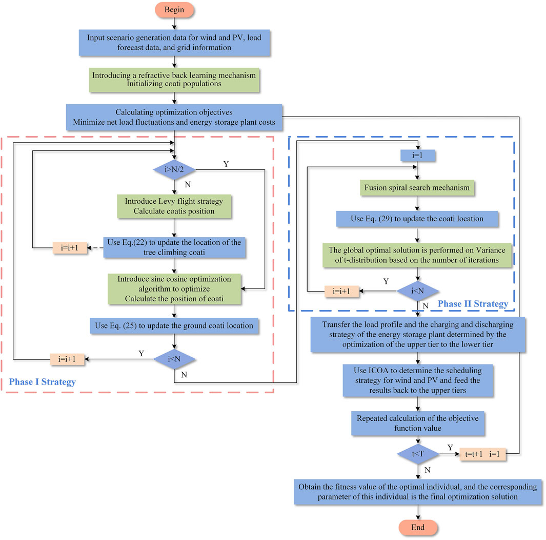
FIGURE 5. Flow chart of the two-tier coordinated optimal scheduling algorithm.

Step 1. Initialization of basic parameters. Initialize the basic data and basic parameters of the algorithm, such as the number of iterations of Improved Coati optimization algorithm and the initial population size.

Step 2. Population initialization. Initialize the coati population, introduce the reflexive learning mechanism, and use the fitness function to evaluate the merits of the individuals generated in Step 1 to find the optimal individual positions.

Step 3. Optimization search in Phase I. Introduce the Levy flight and sine–cosine optimization algorithm in Phase I of ICOA to improve the original ICOA strategy and find the optimal individual position.

Step 4. Optimization search in Phase II. In Phase II of ICOA, fuse the spiral search mechanism and the t-distribution variation mechanism to find the optimal individual position.

Step 5. Upper and lower model interactions. Transfer the charging and discharging strategies and load profiles of the upper-tier energy storage plants to the lower-tier plants. Use the upper-tier transfer results to initialize the lower-tier parameters. Optimize the scheduling strategies of wind power and PV, and feedback the output of wind power, PV, and hydropower units to the upper tier.

Step 6. Iterative optimization. Judge whether the output requirements are met, and if the termination iteration requirements are met, output the optimized scheduling plan before the output day; if not, return to Step 3.

5 Example analysis

5.1 Training of wind power and PV scene generation models based on improved GAN

In this paper, the training and validation datasets are constructed using the Wind1 and PV2 integrated power generation data from NREL for the period of June 2017–June 2018. The dataset contains 52 wind farms and 32 PV plants with a raw data resolution of 5 min, which is cleaned by data cleaning; 80% of them are used as the training set, and the remaining 20% are used as the test set. The improved GAN model is built based on the deep learning framework PyTorch, and the GPU is called for CUDA parallel computing to accelerate the model training. The computer specifications are as follows: 11th Gen Intel(R) Core(TM) i5-1135G7 2.40GHz CPU, 16GB memory, and GPU NVIDIA GeForce MX450 with 16 GB of video memory. The effectiveness of the proposed scene generation method in this paper is first verified. Then, the improved GAN method is compared with the traditional scene generation method for simulation.

Figure 6 shows the loss function and the Wasserstein distance variation profile of the discriminator during the training process. It can be observed that in the initial stage of training, the discriminator loss function increases rapidly due to the inaccurate fitting of the discriminator to the Wasserstein distance. As the number of trainings increases, the overlap between the real and generated sample distributions gradually becomes larger. The Wasserstein distance between the sample distributions decreases. The discriminant loss function gradually changes from an upward trend to a downward trend and tends to be stable, and the network training converges at this time.

FIGURE 6

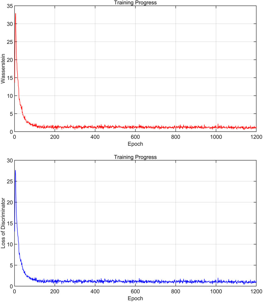
FIGURE 6. Loss function and Wasserstein distance variation profile of the discriminator during training.

A label indicating additional conditions is added to each training sample during training, guiding the generation of scenes with different features. The meanings of the specific condition labels in this paper are shown in Tables 2, 3. The wind scene labels are developed based on the mean size of the daily output relative to the maximum value of the output. The PV scene labels are developed based on the natural month, corresponding to the sampling interval.

TABLE 2

TABLE 2. Wind power sampling interval and its corresponding labels.

TABLE 3

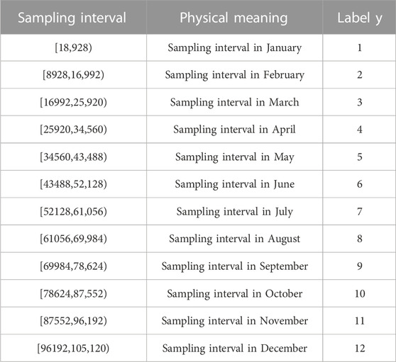
TABLE 3. PV sampling interval and its corresponding labels.

The PV 1 label and the wind power 1 label correspond to the typical scene generation results as shown in Figure 7.

FIGURE 7

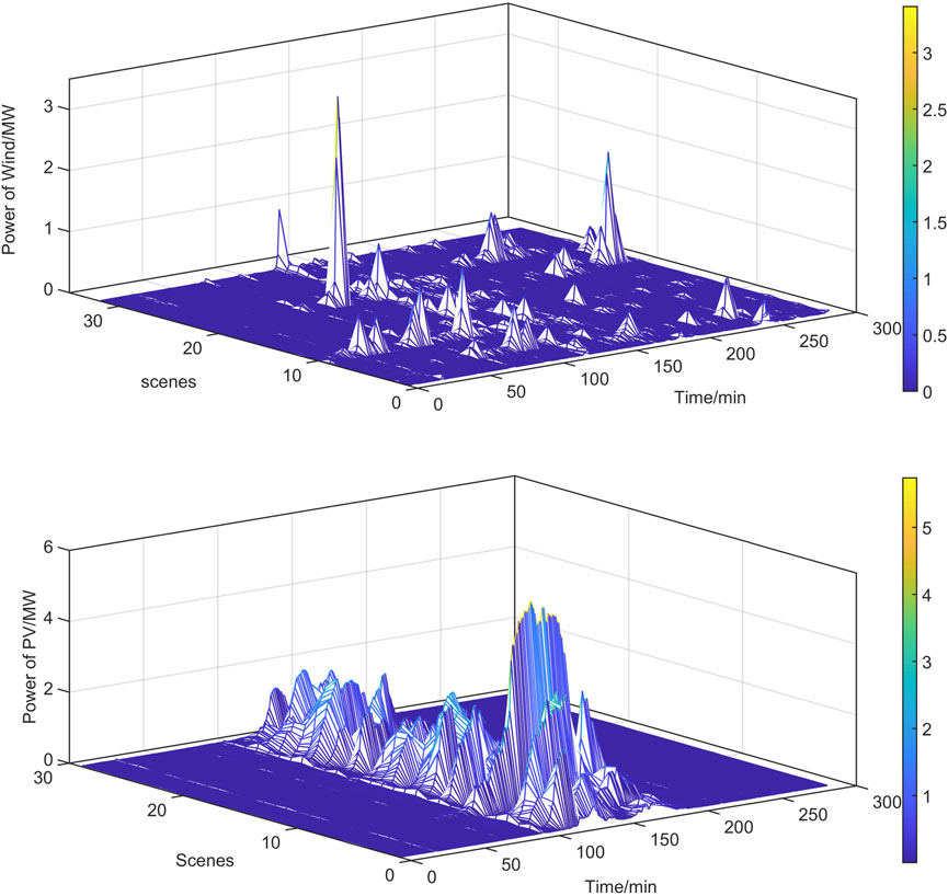
FIGURE 7. Scenarios for label 1 generation for photovoltaic and wind power generation.

The comparison results of cumulative probability distributions of PV and wind power scenes under different methods are shown in Figure 8, respectively, where beta distribution simulation is used for conventional PV and Weibull distribution simulation is used for wind power. From Figure 8, the proposed method fits better with the cumulative probability distributions of real scenarios of PV and wind power. It can reflect the randomness and volatility of historical PV and wind power output data more accurately.

FIGURE 8

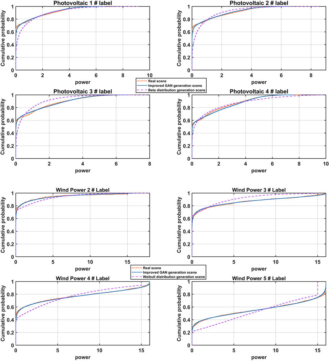
FIGURE 8. Comparison of the cumulative probability distribution of the PV 1–4 tag-out scene and the wind power 2–5 label output scene.

In order to verify the effectiveness of the generated scene using the proposed method, the statistical characteristics between the generated scene and the real sample are compared and illustrated. Table 4 shows the evaluation indexes of the PV June-generated output sample and the real output sample for comparison. As can be observed from Table 4, compared with the traditional method (PV obeys beta distribution), the proposed method is closer to the real sample in two indicators of mean and standard deviation. It can better simulate the volatility of PV output samples over different time periods. Meanwhile, the RMSE and MAE indexes of the proposed method are better than those of the traditional method, which improves the accuracy of PV scene generation.

TABLE 4

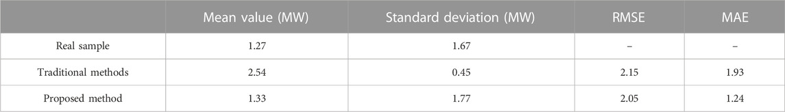
TABLE 4. Evaluation indicators for different models.

5.2 Day-ahead scheduling analysis with wind/PV/hydropower and energy storage systems

5.2.1 Optimized parameter settings

A modified IEEE 30-bus system is used for arithmetic analysis. The system includes four hydropower units, two wind farms, two PV plants, and one energy storage plant. The system structure is shown in Figure 9. The energy storage power station is connected to bus 2, the PV power station is connected to bus 7, and the wind farm is connected to bus 8. The summer solstice day with the maximum system load operation mode is taken as the typical day of load, and the wind power and PV generate the output profile, as shown in Figure 10. The parameters of the upper model are set as follows: the charging and discharging efficiency of both energy storage power plants is 95%; the maximum charging and discharging power is 50 MW; the upper and lower limits of the charge ratio are 0.9 and 0.2, respectively; the rated capacity of the wind farm is 100 MW; and the rated capacity of the PV power plant is 80 MW.

FIGURE 9

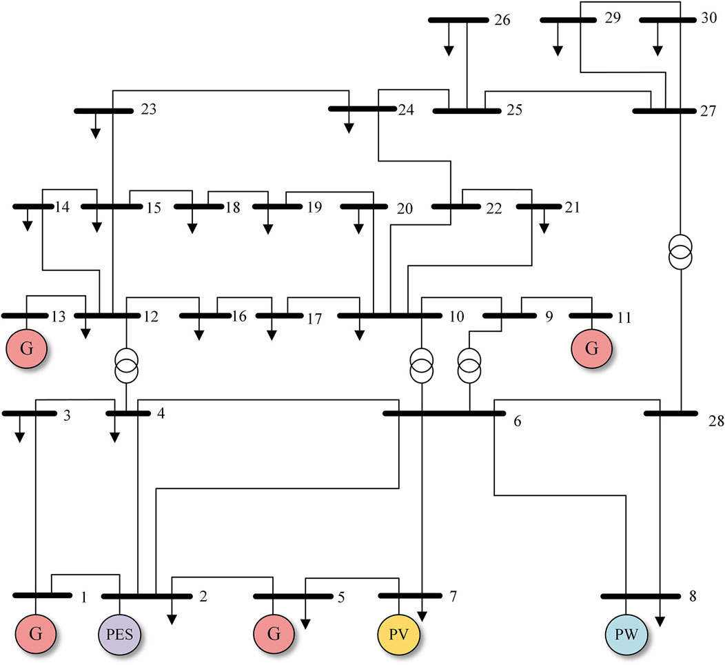
FIGURE 9. Improved IEEE 30-bus system architecture diagram.

FIGURE 10

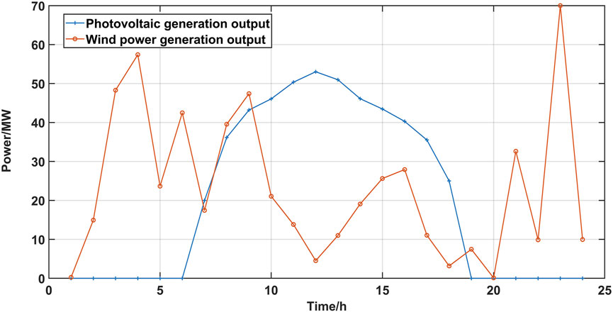
FIGURE 10. Wind and PV power profiles.

5.2.2 Optimized scheduling comparison

The optimal output strategy of the energy storage system and the system load fluctuation are obtained from the upper-tier optimization. The load profiles before and after optimization are shown in Figure 11. It can be observed that the peak-to-valley difference of the optimized system load profile becomes smaller. The load distribution before and after optimization is provided in Table 5. The difference between peaks and valleys of load changes decreased from the initial 170.04 MW to 140.05 MW, representing a decrease of 17.63%. In particular, the peak load is reduced from 283.4 MW to 261.5 MW, and the valley load is increased from 113.36 MW to 121.45 MW. The peak–valley difference before and after optimization changes from 60% to 53.56%, and the load fluctuation rate decreases from 9.45% to 7.97%. The optimization strategy based on the load profile can effectively reduce the overall load fluctuation. Energy storage plants can smooth the overall load profile of the system, reduce the peak-to-valley difference of the load, and realize “peak shaving and valley filling.”

FIGURE 11

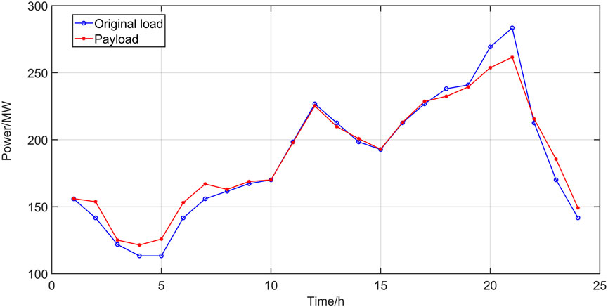
FIGURE 11. Comparison of original load and load profiles.

TABLE 5

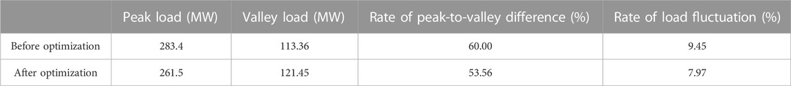
TABLE 5. Distribution of load before and after optimization.

The charge/discharge and charge state changes in the optimized energy storage system are shown in Figure 12. The scheme controls the charge and discharge states of the energy storage system in order to compensate for the anti-peaking characteristics of wind power. It can reduce the output of the hydropower unit and bring some environmental benefits. As can be observed from Figure 12, the storage system starts charging at low load from 1:00 a.m. to 6:00 a.m. and from 3:00 p.m. to 6:00 p.m. to increase the “valley” of the load profile. In the peak hours of 10:00 a.m. to 2:00 p.m. and 7:00 p.m. to 10:00 p.m., the storage system starts to discharge to reduce the “peak” of the load profile. At the same time, the energy storage system is also charged during the “non-valley” hours from 7:00 a.m. to 11:00 a.m. during daytime and during the “non-peak” hours from 10:00 p.m. to 12:00 p.m. in order to increase the consumption capacity of PV. The charging ratio always meets the energy storage operating constraints during the scheduling process. The upper-tier optimal scheduling can effectively relieve the peaking pressure of hydropower units and leave sufficient margin for improving the consumption rate of wind power and PV.

FIGURE 12

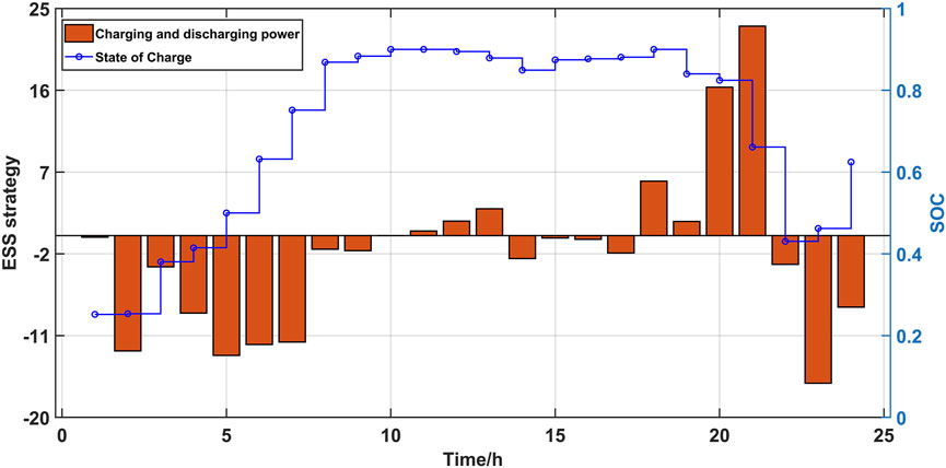
FIGURE 12. Charging and discharging strategies and charge state of energy storage systems.

The power output of each new energy generation system is shown in Figure 13. It can be observed from Figure 13 that the highest wind power grid consumption rate is concentrated during 3:00 a.m.–4:00 a.m. and at 9:00 p.m. It is mainly due to the charging of energy storage plants in the upper optimization during this time, which provides space for the wind power to be consumed. At the same time, the wind power consumption increases at 11:00 p.m. The wind power output reaches its peak at 11:00 p.m., so the wind power consumption capacity is also increased at that time after optimized scheduling. PV grid-connected consumption is concentrated during the period from 6:00 a.m. to 5:00 p.m. during the daytime. The number of starts and stops of hydropower units was reduced to 0. It can maintain a good economy while supplying smooth power to the power system. After optimization, the consumption rate of wind power and PV reaches 66.82%.

FIGURE 13

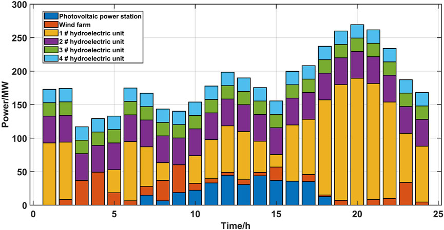
FIGURE 13. Two-tier coordination optimization scheduling strategy.

The comparison of active network loss and grid vulnerability is shown in Figure 14. The active network loss of the system is significantly reduced compared to the pre-optimization period. The average network loss is reduced from 7.43 MW to 3.59 MW, indicating a reduction of 51.68%. The system voltage vulnerability is reduced from the initial voltage vulnerability index of 0.391 to 0.389, indicating a reduction of 0.51%.

FIGURE 14

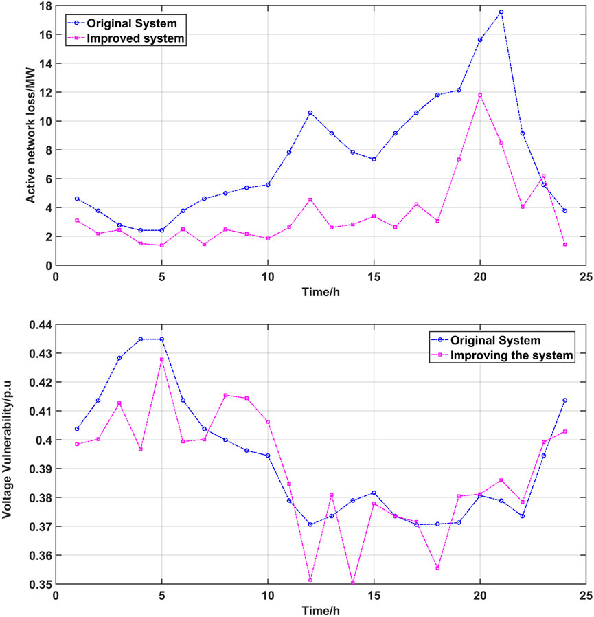
FIGURE 14. Active network loss and voltage vulnerability changes in the system.

5.2.3 Comparison of different scheduling strategies

To verify the economy and effectiveness of the optimization model proposed in this paper, three strategies are selected for comparative analysis.

Case 1. Two-tier optimization model of a power system with wind power/PV/hydropower and energy storage.

Case 2. Two-tier optimization model of a power system with wind power/PV/hydropower and energy storage with all wind power and PV consumed and energy storage considered.

Case 3. Two-tier optimization model of a power system with wind power/PV/hydropower and energy storage without access to energy storage.

All three strategies are based on the new energy generation output and typical daily load profile. The upper and lower optimization objectives of Cases 2 and 3 are the same as those of Case 1. The comparison of the calculation results of the three strategies is shown in Table 6. As can be observed from Table 6, the system load fluctuation rate of Case 1 is the smallest, at only 7.97%. The strategy gives full play to the “low storage and high discharge” function of the grid-connected energy storage power plant. It effectively reduces the peak-to-valley difference of load on the grid. It not only brings certain environmental benefits but also reduces the difficulty in system peak regulation. In Case 2, it results in the full consumption of wind and PV when the overall system load fluctuates due to the wind power anti-peak characteristics. The fluctuation rose from the initial 9.45% to 12.81%, and the load fluctuation rate increased by 35.56%. In Case 3, the fluctuation of the load remains consistent with the fluctuation of the initial load since there is no participation of energy storage plants in the upper objective function.

TABLE 6

TABLE 6. Optimization results for loads under different strategies.

Table 7 provides a comparison of the economic indicators under different operation strategies, where the system operation cost of Case 1 is 34052.35 yuan, which is 22.47% lower compared to 43921.92 yuan of Case 3. The system benefit of Case 2 exceeds its operation and maintenance costs, making the system operation cost result in a negative value in numerical terms, i.e., a profitable trend. This is due to the setting of simulation parameters that can provide environmental benefits to the system.

TABLE 7

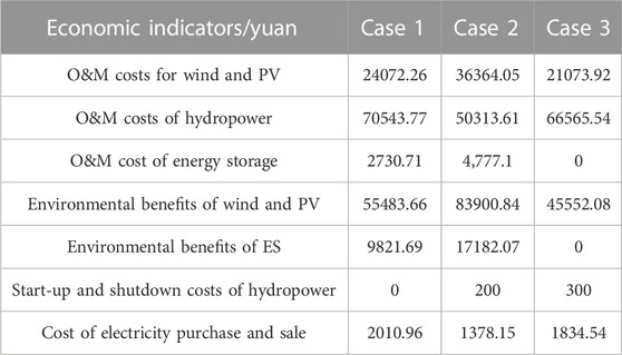
TABLE 7. Economic indicators under different models.

The optimal consumption strategies and consumption rates of wind power and PV power generation are shown in Figure 15. It can be observed that it fails to reduce the load fluctuation of the system because there is no energy storage involved in the system operation in Case 3. It does not ensure the stability of the system, and there is not enough space for the consumption of wind power and PV. The consumption rate of wind power and PV can only reach 54.30%, which is 17.90% lower than the 66.14% in Case 1. It also reduces the revenue of energy storage plants in the system. Among the three strategies, it can better take into account the fluctuation of the system while maintaining a good consumption rate in Case 1, which can effectively improve the economy of the system.

FIGURE 15

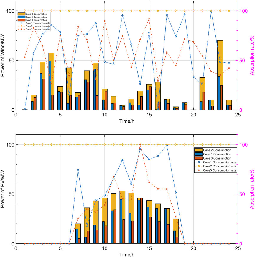
FIGURE 15. Comparison of the best scheduling scheme and consumption rate of wind power and PV plants under different strategies.

Table 8 provides a comparison of the tidal current risk indicators between the three strategies. It can be observed that Case 2 voltage vulnerability index is the lowest, which is reduced by 0.51% and 3.73% compared to 0.389 and 0.402 in Cases 1 and 3, respectively. The active network loss ratio is 3.75% in Case 3, which is reduced by 13.99% and 21.88% compared to the active network loss index of 4.36 and 4.80 in Cases 1 and 2, respectively. It achieves a balance between active network loss and voltage vulnerability (Case 1) and provides a reference for the scheduling of safe and stable operation of the system.

TABLE 8

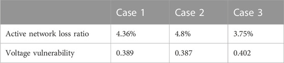
TABLE 8. Trend risk indicators under different strategies.

6 Conclusion

In order to increase the consumption of renewable energy, a two-tier coordinated optimal dispatch model of power systems containing wind/PV/hydropower and energy storage is proposed in this paper. The upper tier aims at minimizing the load fluctuation rate and the cost of energy storage plants. It uses an energy storage system to smooth the load fluctuation of the grid and enhance the consumption capacity of wind power and PV. The lower tier takes the minimum system operation cost and the lowest tidal current risk as the optimization objectives. The purpose of the proposed method is to obtain the optimal scheduling strategy for wind power and PV based on the results of hydroelectric unit scheduling. Furthermore, an improved GAN wind power and PV scenario generation method is proposed. Based on the analysis of the output characteristics of wind power and PV, an improved network structure based on unsupervisedly learned mapping is applied to generate the output operational scenario of wind power and PV. The generation scenarios are effective for coping with the randomness and volatility of wind power and PV. Traditional COA is improved in five parts to accelerate convergence speed and applied to the optimization scheduling problem. Simulation results show that the proposed method can reduce the load fluctuation of the system and increase the consumption of renewable energy.

Data availability statement

The raw data supporting the conclusion of this article will be made available by the authors, without undue reservation.

Author contributions

CC: funding acquisition, supervision, and writing–review and editing. YL: writing–original draft, conceptualization, and methodology. YH: writing–original draft, data curation, and formal analysis. LG: funding acquisition and writing–review and editing.

Funding

This work was supported in part by the Changzhou Sci & Tech Program (CJ20220245), the National Natural Science Foundation of China under Grant 51607057, Jiangsu Key Laboratory of Power Transmission & Distribution Equipment Technology (2021JSSPD07).

Conflict of interest

LG is employed by the company State Grid Shanghai Municipal Jinshan Electric Power Company Limited.

The remaining authors declare that the research was conducted in the absence of any commercial or financial relationships that could be construed as a potential conflict of interest.

Publisher’s note

All claims expressed in this article are solely those of the authors and do not necessarily represent those of their affiliated organizations, or those of the publisher, the editors, and the reviewers. Any product that may be evaluated in this article, or claim that may be made by its manufacturer, is not guaranteed or endorsed by the publisher.

References

An, Y., Zhao, Z., Wang, S., Huang, Q., and Xie, X. (2020). Coordinative optimization of hydro-photovoltaic-wind-battery complementary power stations. CSEE J. Power Energy Syst. 6 (2), 410–418.

Google Scholar

Gejirifu, D., “Dispatching strategy of joint wind, photovoltaic, thermal and energy storage considering utilization ratio of new energy,” Proceedings of the 2022 4th international conference on smart power & internet energy systems (SPIES), Beijing, China, December 2022, pp. 1655–1660.

Google Scholar

Guan, L., Wen, B., Zhan, X., Zhou, B., and Zhao, W., “Scenario generation of wind power based on longitudinal-horizontal clustering strategy,” Proceedings of the 2018 IEEE innovative smart grid technologies - asia (ISGT asia), Singapore, May 2018, pp. 934–939.

Google Scholar

Hounnou, A. H. J., Dubas, F., Fifatin, F. -X., Aza-Gnandji, M., Chamagne, D., and Vianou, A. “Multi-objective optimization of run-of-river small hydro-PV hybrid power systems,” in Proceedings of the 2019 IEEE africon, Accra, Ghana, September 2019, 1–7.

Google Scholar

Hu, C., Luo, Z., Zhou, S., Xie, H., and Hu, L. “Optimal dispatch model of wind power accommodation in combined heat and power system based on unit commitment,” in Proceedings of the 2019 IEEE innovative smart grid technologies - asia (ISGT asia), Chengdu, China, May 2019, 1834–1839.

Google Scholar

Huang, H., Xu, D., Cheng, Q., Yang, C., Lin, X., and Tang, J., “Latin hypercube sampling and spectral clustering based typical scenes generation and analysis for effective reserve dispatch,” Proceedings of the 2022 4th international conference on power and energy Technology (ICPET), Beijing, China, July 2022, pp. 1334–1338.

Google Scholar

Jiang, C., Mao, Y., Chai, Y., Yu, M., and Tao, S. (2018). Scenario generation for wind power using improved generative adversarial networks. IEEE Access 6, 62193–62203. doi:10.1109/access.2018.2875936

CrossRef Full Text | Google Scholar

Jithendranath, J., and Das, D. (2020). Stochastic planning of islanded microgrids with uncertain multi-energy demands and renewable generations. IET Renew. Power Gener. 14 (19), 4179–4192. doi:10.1049/iet-rpg.2020.0889

CrossRef Full Text | Google Scholar

Liang, Z., Chen, H., Chen, S., Lin, Z., and Kang, C. (2019). Probability-driven transmission expansion planning with high-penetration renewable power generation: A case study in northwestern China. Appl. Energy 255, 113610. doi:10.1016/j.apenergy.2019.113610

CrossRef Full Text | Google Scholar

Liu, Z., Xiao, Z., Wu, Y., Hou, H., Xu, T., Zhang, Q., et al. (2021). Integrated optimal dispatching strategy considering power generation and consumption interaction. IEEE Access 9, 1338–1349. doi:10.1109/access.2020.3045151

CrossRef Full Text | Google Scholar

Sadek, S. M., Omran, W. A., Hassan, M. A. M., and Talaat, H. E. A. (2021). Data driven stochastic energy management for isolated microgrids based on generative adversarial networks considering reactive power capabilities of distributed energy resources and reactive power costs. IEEE Access 9, 5397–5411. doi:10.1109/access.2020.3048586

CrossRef Full Text | Google Scholar

Sezer, N., Biçer, Y., and Koç, M. (2019). Design and analysis of an integrated concentrated solar and wind energy system with storage. Int. J. Energy Res. 43 (8), 3263–3283. doi:10.1002/er.4456

CrossRef Full Text | Google Scholar

Wang, C., Ju, P., Wu, F., Lei, S., and Pan, X. (2022). Long-term voltage stability-constrained coordinated scheduling for gas and power grids with uncertain wind power. IEEE Trans. Sustain. Energy 13 (1), 363–377. doi:10.1109/tste.2021.3112983

CrossRef Full Text | Google Scholar

Wang, K., Ren, M., Qian, T., Li, X., Pei, L., and Zhang, X., “Renewable scenario generation based on improved generative adversarial networks,” Proceedings of the 2021 IEEE 5th conference on energy internet and energy system integration (EI2), Taiyuan, China, October 2021, pp. 3155–3159.

Google Scholar

Xia, S., Ding, Z., Du, T., Zhang, D., Shahidehpour, M., and Ding, T. (2020). Multitime scale coordinated scheduling for the combined system of wind power, photovoltaic, thermal generator, hydro pumped storage, and batteries. IEEE Trans. Industry Appl. 56 (3), 2227–2237. doi:10.1109/tia.2020.2974426

CrossRef Full Text | Google Scholar

Yang, B., Cao, X., Cai, Z., Yang, T., Chen, D., Gao, X., et al. (2020). Unit commitment comprehensive optimal model considering the cost of wind power curtailment and deep peak regulation of thermal unit. IEEE Access 8, 71318–71325. doi:10.1109/access.2020.2983183

CrossRef Full Text | Google Scholar

Yang, D., Zhang, C., Jiang, C., Liu, X., and Shen, Y. (2021). Interval method based optimal scheduling of regional multi-microgrids with uncertainties of renewable energy. IEEE Access 9, 53292–53305. doi:10.1109/access.2021.3070592

CrossRef Full Text | Google Scholar

Zhang, Q., Xie, J., Pan, X., Zhang, L., and Fu, D. (2021). A short-term optimal scheduling model for wind-solar-hydro-thermal complementary generation system considering dynamic frequency response. IEEE Access 9, 142768–142781. doi:10.1109/access.2021.3119924

CrossRef Full Text | Google Scholar

Zhang, X., Ma, G., Huang, W., Chen, S., and Zhang, S. (2018). Short-term optimal operation of a wind-PV-hydro complementary installation: yalong river, sichuan province, China. Energies 11 (4), 868. doi:10.3390/en11040868

CrossRef Full Text | Google Scholar

Zhang, X., and Wang, H. “Hierarchical and distributed optimal dispatch for coupled transmission and distribution systems considering wind power uncertainty,” in Proceedings of the 2018 IEEE international conference on energy internet (ICEI), Beijing, China, May 2018, 140–145.

Google Scholar

Zhao, J., Ma, Y., Liu, Q., Wen, L., Jia, C., and Fang, Y. (2020). A multi-source coordinated optimal operation model considering the risk of nuclear power peak shaving and wind power consumption. IEEE Access 8, 189702–189719. doi:10.1109/access.2020.3027705

CrossRef Full Text | Google Scholar