Data-driven methods for situation awareness and operational adjustment of sustainable energy integration into power systems

In the context of increasing complexity in power system operations due to the integration of renewable energy sources, two main challenges arise: accurate short-term wind power forecasting and power flow convergence control. Accurate wind power forecasting plays a crucial role in power system scheduling, while controlling power flow convergence is essential for system stability. This study proposes a concise short-term wind power generation prediction model that combines a feature selection-based convolutional neural network-bidirectional long short-term memory network (CNN-BiLSTM) model. By effectively screening multidimensional feature datasets, the model optimizes the selection of highly correlated feature parameters and assigns weights to input data based on feature correlation. The CNN-BiLSTM combination model is then employed to establish a predictive model for wind power generation based on multiple features. Additionally, this study introduces an automatic adjustment model for power flow convergence using the D3QN (Double Dueling Q Network) reinforcement learning algorithm. This addresses the challenge of power imbalance leading to flow non-convergence, enabling effective control of power flow convergence and adaptive adjustment of operating modes. Experiments conducted using the KDD Cup 2022 wind power prediction dataset validate the wind power prediction method. The results demonstrate that the CNN-BiLSTM model effectively utilizes time-series data, surpassing other neural networks in prediction accuracy. Simulation results based on the PYPOWER case39 standard case reveal that the reinforcement learning model’s reward value increases with training rounds and stabilizes at 40. Remarkably, more than 72% of abnormal flow samples achieve rapid convergence within 10 steps, affirming the proposed method's efficacy and computational efficiency. The findings of this study contribute to enhancing the accurate awareness of new energy integration into power systems and provide a novel adaptive control method for power flow.

1 Introduction

Wind power generation has been widely applied around the world due to its superior environmental benefits, flexible installation scale, and low operation and maintenance costs. As of November 2021, the installed capacity of China’s wind power grid has exceeded 300 million kilowatts, accounting for approximately 13% of the total installed capacity of the country’s power sources, making wind energy one of the important sources of electricity in China.

In recent years, China’s development and utilization of sustainable energy has been rapidly expanding. In March 2021, China proposed deepening the reform of the power system and building a new power system dominated by new energy as a key measure to achieve carbon peaking by 2030. This means that in the future power system, wind and solar power will serve as the main energy sources, while thermal power will serve as a supplementary energy source. However, the high proportion of new energy integration has made the operation characteristics of the power system more complex, and the adjustment and optimization of power system flow are facing unprecedented challenges.

Wind energy has many uncertain factors in practical applications (Wu et al., 2018; Li et al., 2021; Gevorgian et al., 2022; Yan et al., 2023). Without accurate wind energy forecasting, it will pose a huge challenge to the scheduling and management of the power system, and pose a great threat to the stability of the power system. Therefore, in order to ensure the safe and economical operation of large-scale wind power integration, improving the wind power forecasting accuracy of wind farms has become a key issue for the current power system.

Wind power prediction can currently be divided into long-term, short-term, and ultra-short-term prediction based on the time scale (Yang et al., 2018). Different time scales are suitable for different scenarios. Long-term prediction is based on an annual unit and is commonly used to estimate the annual power generation of a wind farm after it is built. Short-term prediction is based on a daily unit and is mainly used for electricity prediction within 2 or 3 days. Ultra-short-term prediction is based on minutes or hours as the prediction unit, and the time resolution is no less than 15 min, which is generally suitable for real-time dispatch of the power system. The significance of ultra-short-term prediction is that it helps optimize the coordination of units and economic dispatch of loads online, as well as optimize the adjustment of frequency and spinning reserve capacity. Because of the extreme specificity of ultra-short-term power prediction, it puts higher requirements on both the prediction time and accuracy.

In the field of short-term power forecasting, various influencing factors exhibit strong regularity and are easily extractable, which provides the possibility for accurate predictions. There are already techniques, such as machine learning-based forecasting methods, including artificial neural networks (ANNs), support vector machines (SVMs), and extreme learning machines (ELMs) (Sun et al., 2014; Portelinha and Tortelli, 2015; Wei et al., 2016; Huimin et al., 2018; Zendehboudi et al., 2018; Fu et al., 2019). Deep learning algorithms can extract and retain data features more comprehensively compared to machine learning algorithms, resulting in better adaptability of prediction models (Overbye, 1994) used wavelet transformation to decompose data sequences and then adopted a targeted learning approach using convolutional neural networks (CNNs) (Overbye, 1995) proposed a wind power uncertainty analysis method based on a Gaussian mixture model and long short-term memory (LSTM). CNNs and LSTMs, with their strong ability to process time series, have already achieved success in short-term power forecasting in various temporal contexts. However, when facing long time series or multidimensional input data, single CNN or LSTM networks still suffer from issues such as incomplete collection of sequence feature information, structural confusion of data between data, and insufficient multidimensional feature mining.

Combining multiple models and methods to predict short-term power can better meet the practical needs of short-term power prediction. This is called a combined model algorithm. Compared with a single model, the generalization ability and prediction accuracy of the combined model have been significantly improved, but there is an overall model entropy increase phenomenon in the process of combining multiple prediction algorithms, which may cause problems such as computational efficiency. Moreover, in practical power systems, power data is often influenced by multi-dimensional feature parameters. To further improve the prediction accuracy of short-term power, the influence of multi-dimensional input feature parameters on short-term power prediction should be taken into consideration.

The attention mechanism uses weight allocation to preserve important information in the input features during training, thus improving the feature extraction ability of the data. Therefore, it can be used as an effective method to improve the accuracy of short-term power prediction. In order to further explore how to improve the performance and prediction accuracy of short-term power prediction models under multi-dimensional input feature parameters, it is necessary to further analyze and optimize the selection of multi-dimensional input feature parameters.

Power flow calculation is the foundation for simulating and analyzing the operation mode and planning of power grids, but convergence issues often arise. As China’s power grid scale expands and loads increase, power flow convergence and adjustment become more difficult. Currently, operators mainly rely on experience to adjust power flow data, which is time-consuming and lacks a systematic and effective method (Zhang et al., 2017; Wang et al., 2020). There are several factors that contribute to power flow adjustment difficulty, including algorithms, models, and data. Firstly, power flow calculations often fail to converge, which is becoming more common as the power grid scale and complexity increase (Zhang et al., 2022). Secondly, the nonlinearity of large power grids increases, making power flow adjustment optimization difficult (Li et al., 2006; Hongfu et al., 2018; Gbadega and Sun, 2022). The third factor is the uncertainty of power flow, making traditional adjustment and optimization methods no longer applicable (Sharma and Ganness, 2007; Liu et al., 2017). With the increase of uncertain factors such as power system sources, networks, and loads, uncertainty has become a significant characteristic of power grid operation. Traditional power system power flow adjustment and optimization methods rely on given deterministic values, only for single-section state calculations, and are greatly affected by parameter accuracy, making it difficult to obtain sufficient and comprehensive information about system power flow and unable to meet the constraint requirements of power grid optimization operation under the condition of a high proportion of renewable energy consumption.

Various adjustment strategies have been proposed to improve the convergence of power flow calculation, including the eigenvalue method, sensitivity analysis, optimal power flow, and others (Liu and Li, 2018) proposes the dropout method and sensitivity analysis to identify weak transmission channels and adjust the output of generators and loads for convergence (Zhang et al., 2022) uses the interior point method for optimal power flow to establish an automatic adjustment model based on the voltage magnitude and phase angle attenuation index to address ill-conditioned and infeasible power flow in large power grids. Several researches based on Newton’s method have proposed optimization methods, optimal multiplier method, Levenberg-Marquardt method, homotopy method, and others, to enhance the calculation ability and expand the convergence margin of power flow calculation (Le et al., 1997; Zhihuan et al., 2015; Liu X. et al., 2017b; Samsonov and Kuchanskyy, 2020; Wu et al., 2020; Zhao et al., 2021). The intelligentization of power grid simulation analysis has also led to extensive research, such as reference (Sutton and Barto, 2018), which proposes an adaptive particle swarm algorithm based on fuzzy control theory for optimal power flow in DC power grid. However, some of these methods require human intervention, and their effectiveness is limited in large power grids (Joshi et al., 2021) proposes a method of transforming PQ nodes into PV nodes when the power flow does not converge due to reactive power imbalance and gradually restoring them to determine the nodes that cannot be restored, which provides a basis for reasonable power flow adjustment.

As artificial intelligence technology has advanced, some scholars have begun to explore its application in power flow convergence adjustment. For instance (Gu et al., 2018), developed an intelligent decision-making system for regional power grid operation mode arrangement, based on the logical thinking of power grid operation mode arrangement (Graves and Graves, 2012) used rules from an expert system to adjust power flow, but this method has limitations as it cannot handle all cases where power flow does not converge (Catalão et al., 2009) combined static network equivalence with an expert system to propose a method for adjusting reactive power and voltage on a large-scale power grid. However, these research methods primarily rely on knowledge bases of expert experience to solve the problem of non-convergence of power flow, lacking flexibility and autonomous exploration mechanisms.

Adjusting power flow convergence through power flow calculation involves modifying power flow parameters, receiving feedback based on the resulting power flow state, and making decisions for the next action. This process follows a typical Markov decision process, which can be addressed through reinforcement learning (Zeng and Qiao, 2011; Zhang et al., 2019). Reinforcement learning is a type of semi-supervised learning that differs from general supervised learning in that it guides behavior by interacting with the environment and receiving rewards. The greater the reward, the greater the likelihood of a particular action being taken. Therefore, this paper proposes a power flow convergence adjustment method based on reinforcement learning for situations where power flow calculation does not converge in large power grids. This method ensures both search efficiency and power flow calculation efficiency.

This paper proposes a CNN-BiLSTM model for ultra-short-term wind power prediction by selecting highly correlated feature parameters from multidimensional input data. The model extracts feature vectors using a CNN network and forms high-dimensional prediction feature vector values in a high-dimensional space. The BiLSTM network is used for bidirectional cycle training, ultimately outputting power prediction results. For the problem of unbalanced active power in power grid flow calculations, this paper proposes a feature selection CNN-BiLSTM deep neural network model. Flow adjustment modeling is treated as a Markov process, and the D3QN (Double Dueling Q Network) reinforcement learning algorithm is used to control automatic adjustment of power grid flow convergence. Experiments using KDD Cup2022 wind power data and PYPOWER’s case39 standard example show that the trained model can efficiently restore most abnormal flow samples to normal and has high flow adjustment efficiency.

2 Data-driven grid operational scheduling framework

2.1 Overall structure

The approach presented in this paper for enhancing situational awareness and adjusting operation modes sustainable energy access power systems is composed of two main components: predicting future power grid trends and adapting operation modes. These are supported by a data-driven auxiliary module, as illustrated in Figure 1.

FIGURE 1

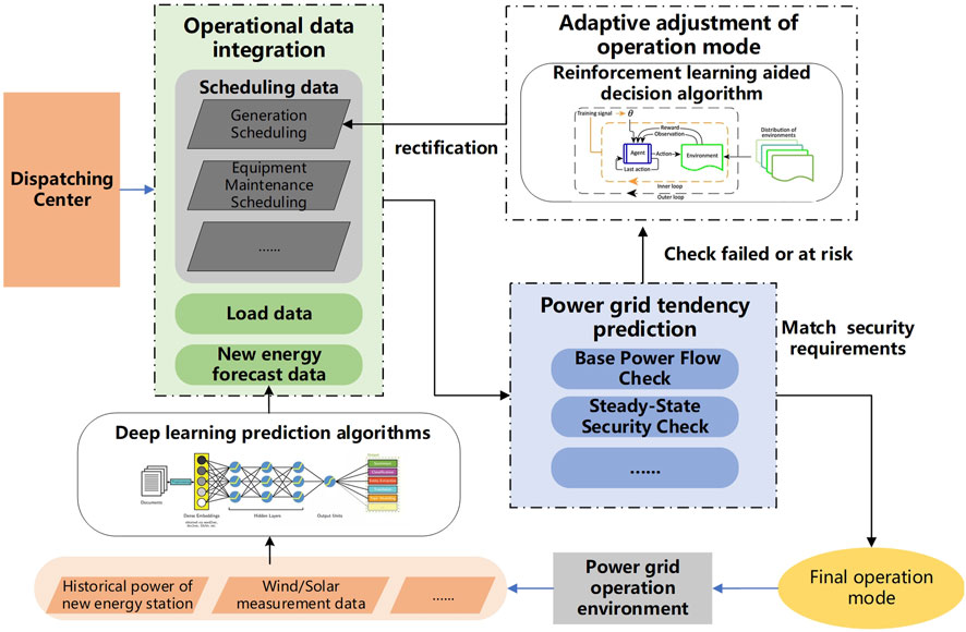
FIGURE 1. Framework for situational awareness and operation mode adjustment of sustainable energy access power system.

The block diagram in Figure 1 illustrates the two links of the proposed method for situational awareness and operation mode adjustment of new energy access power system. In the future trend prediction link of the power grid, planning data such as power generation plans, transmission line plans, and equipment maintenance methods are first collected from the dispatch center. Then, in the data-driven new energy prediction module, the ultra-short-term power prediction of new energy is realized with the support of deep learning technology, based on numerical weather forecasts, actual power of new energy stations, and wind/light measurement data. The new energy data is integrated with load data and planning data to perform safety checks on the operation mode, including basic steady-state flow calculations, static security checks, and other electrical calculations to predict the future trend of the power grid. If safety checks fail or risks exist, such as non-convergence of flow, transmission line power overload, etc., the operation mode adapts and adjusts using deep reinforcement learning for rapid end-to-end adjustment of conventional unit output to formulate power generation plans and operating modes that meet the safety requirements of the power grid.

2.2 Key technologies

2.2.1 Deep learning

Deep learning is a method for learning the intrinsic patterns and hierarchical representations of sample data, including models such as Convolutional Neural Networks (CNNs), Recurrent Neural Networks (RNNs), and Long-Short Term Memory Networks (LSTMs). CNNs are among the most important models in deep learning, inspired by biological cells. For instance, cells beneath the visual cortex are sensitive to local spatial regions, leading to the concept of convolutional kernels. By emulating the neural network between single cells and complex cells, the theory of convolution and down sampling was established. The basic structure of a CNN includes input, convolutional, pooling, fully connected, and output layers. The pooling and convolutional layers are not simply concatenated but are overlapped by connecting some pooling layers to the convolutional layers and then connecting the convolutional layers after the pooling layer. Through such iterative processes, CNNs can maximize the extraction of data features, resulting in efficient and accurate classification and recognition tasks.

The CNN model uses weight sharing and local connectivity to efficiently extract data features through high-dimensional mapping of the original data. During the convolutional layer operation, the CNN network greatly reduces the number of parameters in the training process by locally connecting neurons and weight sharing in the convolutional kernel, which accelerates the model’s training speed. In the pooling layer, the original data is abstracted to reduce feature dimensionality, effectively reducing the number of training parameters and preventing overfitting while improving the model’s generalization ability.

Traditional Recurrent Neural Networks (RNNs) have good performance in processing sequential data. However, as the length of the input sequence increases, the model cannot utilize the earlier data in the sequence, resulting in the problem of long-term dependency. To solve this problem, Hochreiter proposed the Long Short-Term Memory (LSTM) network in 1997 (Zhang J. et al., 2019a). The neural structure of the LSTM network includes three logical units: input gate ${\mathit{i}}_t$, forget gate ${\mathit{f}}_t$, and output gate ${\mathit{o}}_t$, to control the output of memory cells. The input gate controls the input state that enters the memory cell, the forget gate filters the processing result of the previous memory cell, and the output gate controls the output state of the memory cell. In this way, LSTM can effectively handle long-term dependency in the sequence and improve the performance of the model.

The LSTM network calculation process is shown below:

${\mathit{i}}_t=\sigma \left({\mathit{W}}_{\mathrm{i}}{\mathit{x}}_t+{\mathit{U}}_{\mathrm{i}}{\mathit{h}}_{t-1}+{\mathit{b}}_{\mathrm{i}}\right)(1)$

${\mathit{f}}_t=\sigma \left({\mathit{W}}_{\mathrm{f}}{\mathit{x}}_t+{\mathit{U}}_{\mathrm{f}}{\mathit{h}}_{t-1}+{\mathit{b}}_{\mathrm{f}}\right)(2)$

${\mathit{o}}_t=\sigma \left({\mathit{W}}_{\mathrm{o}}{\mathit{x}}_t+{\mathit{U}}_{\mathrm{o}}{\mathit{h}}_{t-1}+{\mathit{b}}_{\mathrm{o}}\right)(3)$

${\stackrel{\sim }{\mathit{c}}}_t=\tanh \left({\mathit{W}}_{\mathrm{c}}{\mathit{x}}_t+{\mathit{U}}_{\mathrm{c}}{\mathit{h}}_{t-1}+{\mathit{b}}_{\mathrm{c}}\right)(4)$

${\mathit{c}}_t={\mathit{i}}_t\circ {\stackrel{\sim }{\mathit{c}}}_t+{\mathit{f}}_t\circ {\mathit{c}}_{t-1}(5)$

${\mathit{h}}_t={\mathit{o}}_t\circ \tanh \left({\mathit{c}}_t\right)(6)$

The value of the input gate ${\mathit{i}}_t$ is determined by the input ${\mathit{x}}_t$, the output of the previous hidden layer ${\mathit{h}}_{t-1}$, and the activation function $\sigma$. The input gate ${\mathit{i}}_t$ is a vector of real numbers between 0 and 1, used to control the degree to which the current input state enters the memory cell. ${\mathit{W}}_{\mathrm{i}},{\mathit{U}}_{\mathrm{i}}$, ${\mathit{b}}_{\mathrm{i}}$, ${\mathit{W}}_{\mathrm{f}}$, ${\mathit{U}}_{\mathrm{f}}$, ${\mathit{b}}_{\mathrm{f}}$, ${\mathit{W}}_{\mathrm{o}},{\mathit{U}}_{\mathrm{o}},{\mathit{b}}_{\mathrm{o}}$ are gate training parameters. Here, $\tanh$ is the activation function.

The hidden layer of LSTM remains in a self-connected form, allowing LSTM to obtain both the cell state and hidden state information from the previous time step. LSTM uses the threshold structure of “forget gate,” “input gate,” and “output gate” to control the replacement and propagation of cell state and hidden state information.

In electrical power parameter prediction, the training is always conducted in a forward manner, which cannot fully explore the intrinsic features of the data and has low utilization of past and future data. BiLSTM uses bidirectional networks to obtain the hidden layer states of the past and future for recursive feedback, so it can explore the intrinsic connections between the current power parameters and the power parameters of past and future time steps, thereby improving the model’s utilization of feature data.

The BiLSTM network model is a combination of forward and backward recurrent structures, in contrast to the traditional LSTM network. In terms of structure, the BiLSTM model adds a data flow from the future to the past in addition to the unidirectional flow from the past to the future of the LSTM network. From a temporal perspective, there is no connection between the hidden layers used for the past and those used for the future in BiLSTM, allowing it to better explore the temporal features of the data.

For the BiLSTM network, the hidden state at each level, ${\mathit{h}}_t$, is composed of three parts: the previous hidden state output, ${\mathit{h}}_{t-1}$, propagating forward along the time axis, the previous hidden state output, ${\mathit{h}}_{i-1}$, propagating backward along the time axis, and the current input quantity, ${\mathit{x}}_t$. The combination process of the hidden states at each level can be represented by Eq. 7:

$\left\{\begin{array}{c}{\mathit{h}}_t=\mathrm{L}\mathrm{S}\mathrm{T}\mathrm{M}\left({\mathit{x}}_t,{\mathit{h}}_{t-1}\right)\\ {\mathit{h}}_i=\mathrm{L}\mathrm{S}\mathrm{T}\mathrm{M}\left({\mathit{x}}_t,{\mathit{h}}_{i-1}\right)\\ {\mathit{h}}_t={\mathit{a}}_t{\mathit{h}}_t+{\mathit{b}}_t{\mathit{h}}_i+{\mathit{c}}_t\end{array}\right.(7)$

The formula represents the computation process of the traditional LSTM network, where ${\mathit{h}}_t$ is the forward hidden state, ${\mathit{h}}_i$ is the backward hidden state, ${\mathit{a}}_t$ is the weight of the forward propagation unit’s hidden state output, bt is the weight of the backward propagation unit’s hidden state output, and ct is the current hidden bias optimization parameter.

2.2.2 Reinforcement learning

Unlike supervised learning, reinforcement learning trains an agent to deal with dynamic environments. The agent reads the environment’s state, takes actions in response, and receives rewards through interaction with the environment, with the goal of maximizing the reward and improving the agent’s action strategy. Compared to traditional dynamic programming methods, reinforcement learning can be modeled based on Markov Decision Process (MDP). Markov Decision Process is the foundation of reinforcement learning modeling and contains five elements: state space S, action space A, transition matrix P, reward function r, and discount factor γ. It can be simply represented as:

$M=<S,A,P,r,\gamma >(8)$

The key to reinforcement learning based on MDP is to learn a policy that maximizes the long-term reward, where each action is taken to achieve the final goal as much as possible. The formula for the long-term reward at time t is as follows:

$R_t={\displaystyle \sum _{k=0}}{\gamma }^k{r}_{t+k+1}(9)$

Deep Reinforcement Learning quantifies the contribution of each action to long-term rewards through a Value Function, thus selecting the most valuable action based on the contribution. The Value Function is defined by the Bellman Equation:

$v_{\pi }\left(s\right)=E_{\pi }\left\{R_t|s_t=s\right\}(10)$

the equation defines the value function $v_{\pi }\left(s\right)$, policy $\pi$, and the main purpose of $v_{\pi }\left(s\right)$ is to measure the value of state $s$.

Most deep reinforcement learning methods train a neural network to approximate the Q-function during the training process, aiming to predict the value of each state-action pair as accurately as possible, and ultimately selecting the action that maximizes the Q-function.

3 Materials and methods

3.1 New energy forecasting based on CNN-BILSTM

3.1.1 CNN-BILSTM network construction

The CNN-BILSTM model used in this study is depicted in Figure 2. The preprocessed data, after feature selection, undergoes feature extraction with one-dimensional convolutional kernels. The dataset is constructed using a sliding time window method and then fed into a BiLSTM neural network. For a given input, the network predicts the power data for the next time step by analyzing the preceding time series data. The filtered data is then inputted into the BiLSTM network for model construction and training. The training and prediction results are then enhanced by the Dense layer to strengthen the data features before output.

FIGURE 2

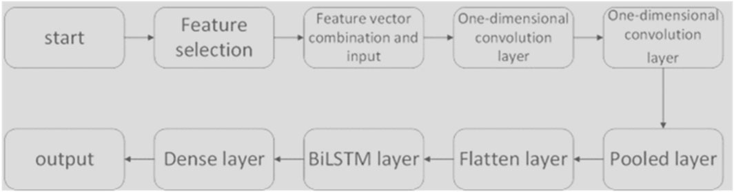
FIGURE 2. CNN-BiLSTM flow chart.

3.1.2 Feature selection and vector weighted combination

Wind power output is often influenced by various factors, such as wind speed, direction, ambient temperature, and blade pitch angle. Predicting wind power output using multidimensional data directly often leads to unsatisfactory results, mainly due to errors in weight allocation for the multidimensional data. Some data have a direct connection with the predicted output, resulting in a higher degree of fit, while other data have a poor degree of fit. When data with high and low degrees of fit are used as inputs to the prediction model, it is difficult to obtain an ideal result. Therefore, this study proposes a method of weighted combination of various feature vectors to balance the imbalance between input data and obtain input data with a high degree of fit. This method is also inclusive when dealing with multidimensional data inputs.

To reduce the algorithm’s generalization error, this paper adopts regularization methods. Regularization strategies involve adding additional parameters as soft constraints to the objective function to reduce generalization errors. Common methods include L2 parameter regularization and L1 parameter regularization. L1 regularization produces a sparser model than L2 regularization. That is, when the L1 regularization is applied to parameters w that are relatively small, it can be reduced to 0, completely excluding irrelevant parameters and greatly assisting feature selection. This technique is also known as LASSO (Zhang et al., 2017).

$\mathrm{\Omega }\left(\theta \right)=\parallel w{\parallel }_1={\displaystyle \sum _i}\left|w_i\right|(11)$

$\nabla w\stackrel{\sim }{J}\left(w;X,y\right)=\alpha \mathrm{s}\mathrm{i}\mathrm{g}\mathrm{n}\left(w\right)+{\nabla }_{w}J\left(w;X,y\right)(12)$

The L1 regularization of model parameters w is controlled by the strength of the positive hyperparameter α.

$J\left(w\right)=\parallel Xw-y{\parallel }_2^2+\alpha \parallel w{\parallel }_1(13)$

${\nabla }_{w}J\left(w\right)=2X^{T}Xw-2X^{T}y+\alpha \mathrm{s}\mathrm{g}\mathrm{n}\left(w\right)(14)$

Here, $w={\left[w_1,\cdots ,w_1\right]}^T\in \mathrm{R}\mathrm{d}$ represents the regression coefficient, and solving the above equation is equivalent to minimizing the first regression term.

We can sort the absolute values of the elements in $w_d$ in descending order. For example, if we have six features, the order of regression coefficients would be | $w_1$ |>| $w_2$ |>| $w_3$ |>| $w_4$ |>| $w_5$ |>| $w_6$ |. The larger the absolute value of the regression coefficient, the more important the corresponding feature is. If we need to select three features for the prediction parameter set, we can choose features 1, 2, and 3 based on their importance.

Once we have selected the three features $w_1$, $w_2$ and $w_3$, we can assign weights to W1, W2, and W3 based on their relative importance. The rule is:

$\sqrt{W_1^2+W_2^2{+W}_3^2}=1(15)$

3.1.3 Attention mechanism

The attention mechanism is a unique approach that mimics human visual processing and is currently one of the most important techniques in the field of deep learning. By allocating weights to highlight key information, the attention mechanism ensures that features are not lost during the model training process. As a result, it can more effectively extract features from remote data with relevant time sequences. Therefore, when dealing with long sequence data and multi-dimensional input feature data, the attention mechanism is often introduced to improve the model’s feature extraction capabilities.

3.2 Power flow adjustment based on DQN

Assuming that there are no inherent issues with the trend computing algorithm, the reasons for non-convergence of the trend mainly include: 1) data errors, 2) active power imbalance, and 3) reactive power imbalance. This article only considers the adjustment method for active power imbalance.

To ensure active power balance, it is necessary to balance the active power between the generator and the load, as well as to ensure that the current carrying capacity of transmission lines does not exceed the limit. Generally, the process of regulating active power imbalance involves first reading the current state of the power grid, including the active power of the generator and load, and the current carrying capacity of the transmission lines. Next, based on the current state of the power grid, a power flow adjustment action is taken and applied to the power grid to change its state. The process of power flow adjustment can be modeled as a Markov decision process (MDP), in which the state space, action space, and reward function need to be designed according to the environment.

3.2.1 State space

Considering the requirement of balancing the active power between generators and loads, and ensuring that the transmission lines are not overloaded, the state space for the flow adjustment of active power imbalance is given by Eq. 17:

$s_t=\left[{\mathit{P}}_{Gen,t},{\mathit{P}}_{Load,t},{\mathit{P}}_{Line,t}\right](16)$

where ${\mathit{P}}_{Gen,t}$ is the active power of the generator at time t, ${\mathit{P}}_{Load,t}$ is the active power of the load at time t, and ${\mathit{P}}_{Line,t}$ is the active power of the transmission line at time t.

3.2.2 Action space

In terms of the flow adjustment action for active power imbalance, this paper only considers adjusting the power of the generator. However, since the power of the generator is continuous, to reduce the size of the action space and make the training easier, the action space needs to be discretized. The following formula is used:

$A_t=\left[\Delta P_{G1},\Delta P_{G2},...,\Delta P_{GN},-\Delta P_{G1},-\Delta P_{G2},...,-\Delta P_{GN}\right](17)$

In this formula, $\Delta P_G$ represents the size of the active power adjustment on the generator for each action, which is a fixed value, while $\pm \Delta P_{Gi}$ means increasing or decreasing the active power of generator i. During the flow adjustment process, a generator is selected for adjustment based on the results of the reinforcement learning algorithm, and its active power is increased or decreased by $\Delta P_G$. It should be noted that in the actual adjustment process, the adjusted generator power should not exceed the power limit of the generator itself.

3.2.3 Reward function

The reward function is composed of three parts that evaluate the results of the power flow calculation: whether the generator power is within limits, whether the transmission line’s active power is within limits, and whether the power flow calculation has converged or not. The power flow calculation results in only two possible outcomes: convergence and non-convergence. When convergence is achieved, the agent should receive a positive reward, and when non-convergence occurs, it should receive a negative reward:

$R_1=\left\{\begin{array}{c}{r}_c\mathrm{i}\mathrm{f}\mathrm{c}\mathrm{o}\mathrm{n}\mathrm{v}\mathrm{e}\mathrm{r}\mathrm{g}\mathrm{e}\mathrm{d}\\ r_{nc}\mathrm{e}\mathrm{l}\mathrm{s}\mathrm{e}\end{array}\right.(18)$

where $r_c$ is the reward value when convergence is achieved, and $r_{nc}$ is the reward value when non-convergence occurs.

On the other hand, it is necessary to consider whether the generator power exceeds the limit. Its reward expression is as follows:

$R_2=-{\max (P}_G-P_{G,\mathit{max}},0)-\max \left(P_{G,\mathit{min}}-P_G,0\right)(19)$

where ${\mathit{P}}_{G,\mathit{max}}$ and ${\mathit{P}}_{G,\mathit{min}}$ represent the upper and lower limits of the active power of the generator. When the generator power is between the upper and lower limits, $R_2$ is 0. When the generator power exceeds the limits, $R_2$ is the negative value of the active power that exceeds or falls below that limit.

The power constraint of the transmission line requires that the transmitted active power of the transmission line does not exceed the limit, expressed as follows:

$R_3=-\mathit{max}\left\{{\mathit{P}}_{line}-{\mathit{P}}_{line,\mathit{max}}\right\}(20)$

where ${\mathit{P}}_{line,\mathit{max}}$ represents the maximum active power that can be transmitted through the transmission line.

In the end, the total reward value R obtained is:

$R=R_1+R_2+R_3(21)$

The framework of flow adjustment based on reinforcement learning is shown in Figure 3. The dashed line represents the interaction between the agent and the environment, and the solid line represents the training process of the agent. In the interaction process, the agent reads the state from the environment, obtains the optimal action through the D3QN network, and applies it to the environment. The generated data is stored in the experience replay pool. In the training process, data is randomly sampled from the experience replay pool based on the principle of prioritized experience replay.

FIGURE 3

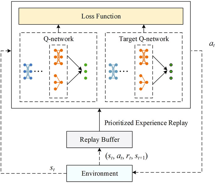
FIGURE 3. Framework for current adjustment based on reinforcement learning.

DQN (Deep Q-Network) is a widely used reinforcement learning algorithm for discrete action prediction. The DQN algorithm uses a Q-network to estimate the Q value. However, training with only one network is relatively unstable and can easily lead to high Q-value overestimation. Therefore, this paper adopts the D3QN (Double Dueling Q Network) reinforcement learning algorithm to automatically adjust the flow convergence of the power grid. D3QN is an improved version of the traditional deep Q network that solves problems such as instability and Q-value overestimation. The active power of the generator, load, and transmission line are used as input, and the Q value of the action under the current state is obtained through a four-layer fully connected network and the advantage and value network.

The final output of the D3QN method is as follows:

$Q^{\pi }\left(s,a\right)=V^{\pi }\left(s\right)+A^{\pi }\left(s,a\right)-\frac{1}{\left|A\right|}{\displaystyle \sum _{a^{\prime }}}{A}^{\pi }\left(s,a^{\prime }\right)(22)$

In the formula, π represents the parameters of the neural network, $Q^{\pi }\left(s,a\right)$ represents the Q value, $V^{\pi }\left(s\right)$ represents the value function, and $A^{\pi }\left(s,a\right)$ represents the advantage function.

The Double Q structure consists of two networks: the Q-network and the target-Q network. The Q-network and the target Q-network will produce the In each parameter update process.

$y_t=\left\{\begin{array}{c}{r}_t\mathrm{i}\mathrm{f}\hspace{0.33em}{s}_{t+1}\hspace{0.33em}\mathrm{i}\mathrm{s}\mathrm{e}\mathrm{n}\mathrm{d}\\ r_t+\gamma Q^{{\pi }^{\prime }}\left(s_{t+1},\mathit{arg}\underset{a}{\mathit{max}}{Q}^{\pi }\left(s_{t+1},a\right)\right)\mathrm{e}\mathrm{l}\mathrm{s}\mathrm{e}\end{array}\right.(23)$

$L={‖y_t-Q^{\pi }\left(s_t,a_t\right)‖}^2(24)$

where $r_t$ represents the reward value, $y_t$ represents the target function, and $L$ represents the loss function.

4 Example verification

4.1 Power system situational awareness prediction

The characteristic data is derived from the KDD Cup 2022 Wind Power generation Forecast dataset, and the SDWPF is provided by Longyuan Power Group Co., LTD. This dataset includes the spatial distribution of the wind turbine, weather, time, and conditions inside the turbine. SCADA data is sampled every 10 min from each of the 134 wind turbines in the wind farm owned by Longyuan Power Group.

For the training and testing set selection, we employed a 70–30 train-test split ratio. Specifically, 70% of the dataset was randomly allocated to the training set, while the remaining 30% was reserved for the testing set. This random splitting ensures that both sets are representative of the overall dataset and avoids potential biases that may arise from a specific ordering of the data.

4.1.1 Feature vector screening and combination

All feature vectors are obtained by using the output sparsity of L1 norm. This paper uses the lasso regression provided by sklearn for calculation. Lasso regression has a regularization parameter alpha, which is used to control the strength of the characteristic variable coefficient being constrained to 0. If the alpha parameter is too large, the constraint ability of the input data is smaller, and it is more difficult to judge the under-fitting of the feature. On the contrary, the smaller the value of the alpha parameter, the stronger the ability to constrain the data, and the more difficult it is to judge the overfitting of the input data. After weighing the pros and cons of the two, this paper chooses alpha = 0.1 as the constraint. In turn, each data is brought into LASSO for calculation, and the regression coefficient $\omega$ of each data is obtained.

The dataset is filtered by L1 regularization. The specific data is shown in Table 1, and the regression coefficient is obtained in Figure 4.

TABLE 1

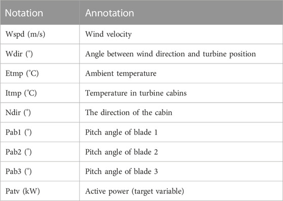
TABLE 1. Data.

FIGURE 4

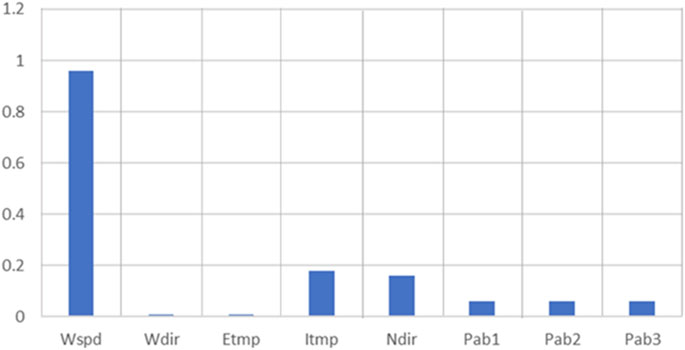
FIGURE 4. Regression coefficient.

According to the regression coefficient, the four vectors with the largest regression coefficient are weighted and combined to form a new prediction vector set. After normalization, the feature data is given corresponding weights, and the new input features are combined.

$data=W_{1}Wspd+W_{2}Ndir+W_{3}Itmp+W_{4}Pab3(25)$

4.1.2 Evaluation index

In this paper, the root mean square error RMSE, which is commonly used in ultra-short-term power prediction, is used as the evaluation index. The calculation methods are as follows:

$d{R}_{\mathrm{M}\mathrm{S}\mathrm{E}}=\sqrt{\frac{{\sum }_{i=1}^N{\left(y_i-y_{\mathrm{f}\mathrm{i}}\right)}^2}{N}}(26)$

$y_i$ is the true value of the sample point i. $y_{\mathrm{f}\mathrm{i}}$ is the predicted value of the sample point i; N is the number of sample points.

In order to ensure the accuracy of the model training and the scientificity of the prediction process, the $R_{\mathrm{M}\mathrm{S}\mathrm{E}}$ and $M_{\mathrm{A}\mathrm{P}\mathrm{E}}$ obtained from the prediction results are the average values calculated after the test set is brought into the data set.

4.1.3 Experimental result analysis

After 16 rounds of calculation, the average loss coefficient of each round in 16 rounds is shown in Figure 5. It can be seen from the diagram that with the increase of training rounds, the validation_loss coefficient decreases continuously, and the loss coefficient finally approaches around 0.005. It can be concluded that the CNN-BiLSTM model based on feature screening proposed in this paper has high accuracy for wind power prediction.

FIGURE 5

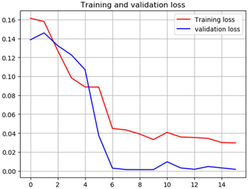
FIGURE 5. Average loss function table.

4.1.4 Comparison between different models

In order to further illustrate the superiority of the CNN-BiLSTM combined model based on feature screening, this paper selects the long and short time memory network LSTM, recurrent neural network RNN, GRU network to process the same data. In order to unify the input variables, the input features are normalized to form a single feature vector and then processed. The root mean square error RMSE and the mean percentage error MAPE are used to evaluate the performance of the model, and the average loss is calculated as shown in Table 2.

TABLE 2

TABLE 2. Average loss.

The comparison between the predicted value and the actual value of wind power generation in the next 1,790 min is shown in Figure 6. It can be seen that the model proposed in this paper can fit the wind power value to a certain extent. By comparing the RMSE values of different models in Table 2, it can be concluded that the CNN-BiLSTM combined model is far superior to other models. The reason for the analysis is that, firstly, other models only perform simple normalization processing when dealing with multi-dimensional feature input, and do not judge the fitting degree of the vectors of each dimension in the multi-dimensional data to the output, resulting in high-fitting vectors. Not prominent enough, low-fitting vectors reduce prediction accuracy. Secondly, other models fail to deal with the impact of past and future data on the present in time series data, and the utilization rate of data is not high enough, resulting in unsatisfactory output accuracy.

FIGURE 6

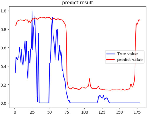
FIGURE 6. Comparison of predicted and actual values of wind power generation in the next 1,790 min.

4.2 Adaptive operation mode adjustment

4.2.1 Example preparation and parameter selection

In order to verify the effect of the proposed method, this paper takes PYPOWER as the platform of power flow calculation, and the power flow calculation method adopts Newton-Raphson method. The application example in this paper is the case39 standard example in PYPOWER. The wiring diagram of the case39 example is shown in Figure 7, which contains 10 generators, 39 nodes and 46 transmission lines. In order to generate non-convergent power flow data for training, the generator and load are randomly changed based on the initial convergence power flow. Among them, No. 2, No. 6, and No. 7 generators are replaced with wind turbines. Its installed capacity and installed capacity are shown in Table 3. During the power flow adjustment, the power data of No. 2, No. 6, and No. 7 wind turbines are predicted by CNN-BiLSTM. The load power is randomly transformed with a certain amplitude. In this way, a total of 2,000 abnormal power flows including non-convergence of power flow, over-limit of generator power and over-limit of load voltage are generated. Among them, 1950 data were selected as the training set, and the remaining 50 data were used as the test set.

FIGURE 7

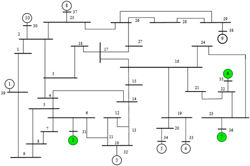
FIGURE 7. PYPOWER case39 example wiring diagram.

TABLE 3

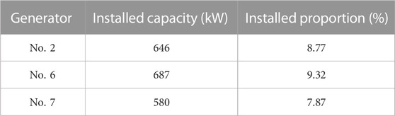
TABLE 3. The installed capacity and proportion of No. 2, No. 6, and No. 7 wind turbines.

Figure 8 shows the number of convergent and non-convergent samples in the 2,000 samples produced as the load ratio increases. It can be seen that when the load increase ratio remains below 1.5 times, the convergence samples account for the majority, and when the load increase ratio comes to 1.6 to 2.0 times, the convergence samples are in the majority. When the ratio is between 1.8 and 2.0, the number of convergence samples is less than 250. At this time, the samples are extremely unbalanced due to the excessive proportion of load increase, which makes it difficult to adjust to convergence. Therefore, the final choice of load ratio is between 1.0 and 1.4 times.

FIGURE 8

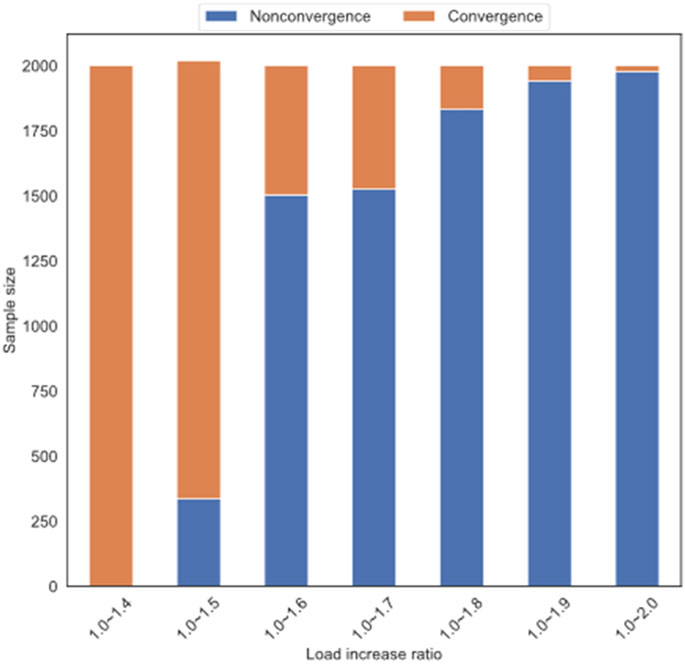
FIGURE 8. The proportion change of convergent and non-convergent power flow.

The parameter selection of D3QN reinforcement learning model is shown in Table 4. In this experiment, the power flow adjustment is required to be completed within 50 power flow adjustment actions, otherwise it is regarded as a power flow adjustment failure. The training environment of this experiment is 11th Gen Intel (R) Core (TM) i7-11800H, RTX 3060,16G memory, using Python 3.9.

TABLE 4

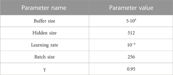
TABLE 4. Parameter selection of D3QN model.

4.2.2 Experiment part

In the above experimental environment, 2000 rounds of training are performed, and every 10 rounds are tested on the test set. The obtained reward value curve is shown in Figure 9. It can be seen that with the increase of training rounds, the reward value obtained also shows an increasing trend. The reward value eventually stabilized at 40. It can be concluded that the D3QN reinforcement learning model used in this paper has a good effect on automatic power flow adjustment.

FIGURE 9

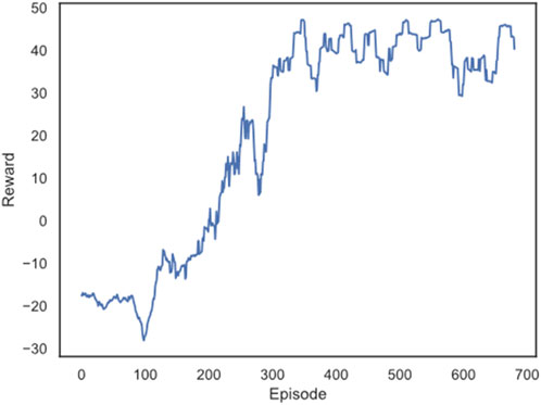
FIGURE 9. The change of the average reward value of the test set with the number of training rounds.

Table 5 shows the performance of the model on the test set. Among them, the samples that restore the normal power flow within 10 steps are recorded as the samples that recover quickly, the samples that restore the normal power flow within 10 steps to 50 steps are recorded as the samples that recover slowly, and the samples that exceed 50 steps are recorded as the samples that do not recover. It can be found that the trained model can restore more than 72% of abnormal power flow samples to normal. This shows that the method proposed in this paper can effectively adjust the automatic power flow and improve the abnormal power flow. On the other hand, the average power flow adjustment time of this model except power flow calculation is only 0.0028 s, which shows that this method has high power flow adjustment efficiency.

TABLE 5

TABLE 5. The performance of the model on the test set.

In order to more accurately illustrate the effect of the proposed method on the automatic power flow adjustment, this experiment selected the fourth sample in the test set, and recorded the change of the generator over-limit power during the power flow adjustment process after the training was completed, as shown in Figure 10. It can be found that during the power flow adjustment process of this sample, the over-limit power of the generator gradually decreases with the continuous adjustment of the power flow, and finally returns to zero in step 7. Therefore, the power flow adjustment algorithm after training can effectively reduce the generator’s over-limit power and make the power flow return to normal. This shows that the method proposed in this paper can effectively reduce the active power limit of the generator, so that the power flow can return to normal.

FIGURE 10

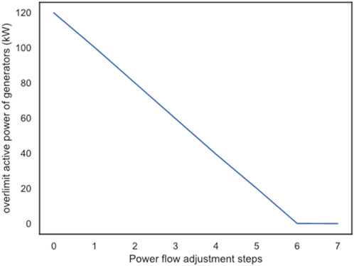
FIGURE 10. The fourth sample of generator over-limit power.

5 Conclusion

In this paper, a combined wind power prediction model considering historical time series and feature screening is proposed based on the research status of wind power prediction and the idea of joint model. Based on the KDD Cup 2022 wind power prediction data set, the validity of the model is verified. Finally, the single model and other methods are compared with the model established in this paper, and the following conclusions are drawn:

(1) The CNN-BiLSTM combined model based on feature screening has high accuracy for short-term and ultra-short-term prediction of wind power, and greatly improves the utilization of time series data. Compared with other models, the model can extract the correlation of multi-dimensional features to the objective function through feature screening, and can give more comprehensive and comprehensive prediction results.

(2) In the face of multi-dimensional data ultra-short-term prediction, the model proposed in this paper has great advantages in solving such problems. It can not only make extensive use of historical data and future data in the data set, but also reduce the problem of algorithm entropy increase caused by multi-feature vectors, which is suitable for the current wind power prediction trend.

On this basis, combined with reinforcement learning algorithm and Markov decision process, this paper proposes an automatic adjustment method for power flow calculation convergence. By adding the constraints of generator and load power balance and transmission line not exceeding the limit in reinforcement learning, the search space is reduced and the search is directional. Through the example analysis, the proposed method can effectively adjust and converge the non-convergent power flow, and realize the automatic adjustment of power flow calculation convergence. The model reward value increases with the increase of the number of training rounds and stabilizes at 40. More than 72% of the samples can converge quickly, that is, the power flow adjustment effect is good and the calculation efficiency is high.

One limitation lies in the validation process, where we only used a single dataset for experimentation. To address this, we commit to conducting future tests on diverse datasets to thoroughly assess the generalization capabilities of our model across different scenarios. By validating our method on multiple datasets, we can provide stronger evidence of its robustness and applicability.

Additionally, in our power flow adjustment experiments, we prioritized time-sensitive data to address convergence challenges. While we successfully demonstrated the effectiveness of our approach, we did not compare it with other existing methods, limiting the understanding of its performance relative to conventional approaches. In light of this, our future work will involve conducting comprehensive comparisons with traditional methods, such as MILP and heuristic techniques. These comparisons will provide valuable insights into the strengths and weaknesses of our data-driven approach in relation to established optimization methods.

Looking ahead, we aim to further improve our proposed method by exploring additional characteristics of active power imbalance and expanding the types of power flow adjustment actions. This research direction will contribute to enhancing the efficiency and effectiveness of power flow adjustment in real-world power systems.

In conclusion, we are committed to refining our wind power prediction model and power flow adjustment method to address the mentioned limitations. By conducting experiments on various datasets and comparing our approach with traditional methods, we aspire to enhance the credibility and broad applicability of our research. Ultimately, our efforts will contribute to the advancement of wind power prediction and power flow adjustment techniques, supporting the development of efficient and sustainable power systems.

Data availability statement

The original contributions presented in the study are included in the article/Supplementary Material, further inquiries can be directed to the corresponding author.

Author contributions

SJ, QL, and WZ contributed to conception and design of the study. ZH organized the database. YXH performed the statistical analysis. LZ wrote the first draft of the manuscript. YL, PX, XZ, and YHH wrote sections of the manuscript. All authors contributed to the article and approved the submitted version.

Conflict of interest

Authors SJ, QL, WZ, ZH, YXH, LZ, YL, XZ, and YHH were employed by State Grid Hubei Electric Power Company.

The remaining author declares that the research was conducted in the absence of any commercial or financial relationships that could be construed as a potential conflict of interest.

Publisher’s note

All claims expressed in this article are solely those of the authors and do not necessarily represent those of their affiliated organizations, or those of the publisher, the editors and the reviewers. Any product that may be evaluated in this article, or claim that may be made by its manufacturer, is not guaranteed or endorsed by the publisher.

References

Catalão, J. P. d. S., Pousinho, H. M. I., and Mendes, V. M. F. "An artificial neural network approach for short-term wind power forecasting in Portugal", in: Proceedings of the 2009 15th International Conference on Intelligent System Applications to Power Systems: IEEE), 1–5.

Google Scholar

Fu, W., Wang, K., Li, C., and Tan, J., (2019). Multi-step short-term wind speed forecasting approach based on multi-scale dominant ingredient chaotic analysis. Improv. hybrid GWO-SCA Optim. ELM 187, 356–377.doi:10.1016/j.enconman.2019.02.086

CrossRef Full Text | Google Scholar

Gbadega, P. A., and Sun, Y. J. E. R. (2022). Primal–dual interior-point algorithm for electricity cost minimization in a prosumer-based smart grid environment: A convex optimization approach, 8, 681–695.

CrossRef Full Text | Google Scholar

Gevorgian, V., Shah, S., Yan, W., and Henderson, G. J. I. E. M. (2022). Grid-Forming Wind: Getting ready for prime time, with or without inverters. 10(1), 52–64.

CrossRef Full Text | Google Scholar

Graves, A., and Graves, A. (2012). Long short-term memory, 37–45.

CrossRef Full Text | Google Scholar

Gu, J., Wang, Z., Kuen, J., Ma, L., Shahroudy, A., Shuai, B., et al. (2018). Recent Adv. convolutional neural Netw. 77, 354–377.

CrossRef Full Text

Hongfu, W., Xianghong, T., and Baiqing, L. J. P. o. t. C. (2018). An approximate power flow model based on virtual midpoint power. 38(21), 6305–6313.

Google Scholar

Huimin, P., Feng, L., Huling, Y., and Yanhong, B. J. (2018). Power flow calculation and condition diagnosis for operation mode adjustment of large-scale Power Syst. J.42(3), 136 doi:10.7500/AEPS20170406004

CrossRef Full Text | Google Scholar

Joshi, D. J., Kale, I., Gandewar, S., Korate, O., Patwari, D., and Patil, S. “Reinforcement learning: A survey,” in Machine learning and information processing: Proceedings of ICMLIP 2020 (Springer), 297–308.

Google Scholar

Le, T. L., Negnevitsky, M., and Piekutowski, M. J. I. t. o. p. s. (1997). Network equivalents and expert system application for voltage and VAR control in large-scale power systems. 12(4), 1440–1445.

PubMed Abstract | Google Scholar

Li, M., Chen, J.-f., and Chen, H.-y. J. A. o. E. P. S. (2006). Load flow regulation for unsolvable cases in a power system. 30 (8), 11–15.

Google Scholar

Li, Y., Gao, W., Huang, S., Wang, R., Yan, W., Gevorgian, V., et al. (2021). Data-driven optimal control strategy for virtual synchronous generator via deep reinforcement learning approach. 9(4), 919–929.

CrossRef Full Text | Google Scholar

Liu, D., He, W., and Zhang, C. (2017). Proceedings of the IEEE 2nd Advanced Information Technology, Electronic and Automation Control Conference. (IAEAC): IEEE), 2442–2446.The research and optimization on levenberg-marquard algorithm in neural net

CrossRef Full Text | Google Scholar

Liu, R., and Li, L. J. (2018). Simulated annealing algorithm coupled with a deterministic method for parameter extraction of energetic hysteresis model. 54(11), 1–5.

CrossRef Full Text | Google Scholar

Liu, X., Wen, J., Pan, Y., Wu, P., and Li, J. J. P. S. T. (2017b). OPF control of DC-grid using improved. PSO algorithm 41 (3), 715–720.doi:10.1016/j.ijepes.2022.108375

CrossRef Full Text | Google Scholar

Overbye, T. (1995). Comput. a Pract. method restore power flow solvability 10 (1), 280–287.

CrossRef Full Text

Overbye, T. (1994). A power flow measure for unsolvable cases. 9(3), 1359–1365.

CrossRef Full Text | Google Scholar

Portelinha, R. K., and Tortelli, O. L. (2015). IEEE PES Innov. Smart Grid Technol. Lat. Am. IEEE, 81–86.Three phase fast decoupled power flow for emerging distribution systems

CrossRef Full Text | Google Scholar

Samsonov, D., and Kuchanskyy, V. J. (2020). Optimization of operation modes bulk electric power grids, 83–85.

Google Scholar

Sharma, C., and Ganness, M. G. "Determination of power system voltage stability using modal analysis", in: Proceedings of the 2007 International Conference on Power Engineering,: IEEE, 381–387.

Google Scholar

Sun, Q., Chen, H., Yang, J., and Yang, J. J. P. (2014). Analysis on convergence of Newton-like power flow algorithm. 34(13), 2196–2200.

Google Scholar

Sutton, R. S., and Barto, A. G. (2018). Reinforcement learning: An introduction. MIT press.

Google Scholar

Wang, T., Tang, Y., Huang, Y., Chen, X., Zhang, S., and Huang, H. (2020). Proceedings of the IEEE 4th Conference on Energy Internet and Energy System Integration (EI2). IEEE, 694–699.Automatic adjustment method of power flow calculation convergence for large-scale power grid based on knowledge experience and deep reinforcement learning

CrossRef Full Text | Google Scholar

Wei, C., Zhang, Z., Qiao, W., and Qu, L. J. I. T. o. P. E. (2016). An adaptive network-based reinforcement learning method for MPPT control of PMSG wind energy conversion systems. 31(11), 7837–7848.

CrossRef Full Text | Google Scholar

Wu, S., Hu, W., Lu, Z., Gu, Y., Tian, B., Li, H. J. J. o. m. p. s., et al. (2020). Power system flow adjustment and sample generation based on deep reinforcement learning. 8(6), 1115–1127.

CrossRef Full Text | Google Scholar

Wu, Z., Gao, W., Gao, T., Yan, W., Zhang, H., Yan, S., et al. (2018). State-of-the-art review on frequency response of wind power plants in power systems. 6(1), 1–16.

CrossRef Full Text | Google Scholar

Yan, W., Gevorgian, V., and Shah, S. (2023). Synchronous wind: Evaluating the grid impact of inverterless grid-forming wind power plants. Golden, CO (United States: National Renewable Energy Lab.

Google Scholar

Yang, M., Chen, X., Du, J., and Cui, Y. J. I. a. (2018). Ultra-short-term multistep wind power prediction based on improved EMD and reconstruction method using run-length analysis. 6, 31908–31917.

CrossRef Full Text | Google Scholar

Zendehboudi, A., Baseer, M. A., and Saidur, R. J. J. o. c. p. (2018). Application of support vector machine models for forecasting solar and wind energy resources. A Rev. 199, 272–285.doi:10.1016/j.jclepro.2018.07.164

CrossRef Full Text | Google Scholar

Zeng, J., Qiao, W., and Year, ). (2011).Proceedings of the IEEE/PES power systems conference and exposition: IEEE), 1–8.Support vector machine-based short-term wind power forecasting

CrossRef Full Text | Google Scholar

Zhang, C., Chen, H., Shi, K., Qiu, M., Hua, D., and Ngan, H. J. I. T. o. S. G. (2017). An interval power flow analysis through optimizing-scenarios method. 9(5), 5217–5226.

Google Scholar

Zhang, C., Ding, M., Wang, W., Bi, R., Miao, L., Yu, H., et al. (2019a). An improved ELM model based on CEEMD-LZC and manifold learning for short-term wind power prediction. 7, 121472–121481.

CrossRef Full Text | Google Scholar

Zhang, J., Luo, S., Xia, C., Zhu, Y., and Xia, R. (Year). "Optimal power flow calculation for wind power grid connection based on adjustable robust optimization theory", in: Proceedings of the 2022 7th Asia Conference on Power and Electrical Engineering : IEEE, 1927–1931.

Google Scholar

Zhang, J., Yan, J., Infield, D., Liu, Y., and Lien, F.-s. J. A. E. (2019b). Short-term forecasting and uncertainty analysis of wind turbine power based on long short-term memory network and Gaussian mixture model. 241, 229–244.

CrossRef Full Text | Google Scholar

Zhao, H., Zhang, J., Wang, X., Yuan, H., Gao, T., Hu, C., et al. (2021). The economy and policy incorporated computing system for social energy and power. Consum. Anal. 13 (18), 10473. doi:10.3390/su131810473

CrossRef Full Text | Google Scholar

Zhihuan, L., Yunfei, H., Yinsheng, S., Xin, S., and River, Y. J.(2015). A convergence adjustment method of power flow based on node type switching. 39(7), 188–193.

Google Scholar