Interval reservoir computing: theory and case studies

The time series data in many applications, for example, wind power and vehicle trajectory, show significant uncertainty. Using a single prediction value of wind power as feedback information for wind turbine control or unit commitment is not enough since the uncertainty of the prediction is not described. This paper addresses the uncertainty issue in time series data forecasting by proposing the novel interval reservoir computing method. The proposed interval reservoir computing can capture the underlying evolution of the stochastic dynamical system for time series data using the recurrent neural network (RNN). On the other hand, by formulating a chance-constrained optimization problem, interval reservoir computing outputs a set of parameters in the RNN, which maps to an interval of prediction values. The capacity of the interval is the smallest one satisfying the condition that the probability of having a prediction inside the interval is lower than the required level. The scenario approach solves the formulated chance-constrained optimization problem. We implemented an experimental data-based validation to evaluate the proposed method. The validation results show that the proposed interval reservoir computing can give a tight interval of time series data forecasting values for wind power and traffic trajectory. In addition, the confidence probability over the feasibility goes to 1 very quickly as the sample number increases.

1 Introduction

Time series data prediction is vital in many applications for pursuing better control or decision-making performance toward achieving a better society or quality of life. For example, to accomplish the net-zero carbon goal, it is vital to establish a reliable power system with renewable energy for energy supplement instead of high-carbon power generation (Evans et al., 2021). Wind energy is one of the best choices among different kinds of renewable energy resources. However, wind power has a stochastic nature, which makes it challenging to realize the optimal wind power supplementation with high reliability (Zhao et al., 2018; Ge et al., 2022). It is necessary to provide a reliable wind power prediction for the security-constrained unit commitment (SCUC) problem to improve the optimality and reliability of wind power supplementation (Hu and Wu, 2016). Instead of using one single wind power prediction, the SCUC problem involved with wind power often considers the uncertain nature of wind power. It is formulated as a stochastic program (Chen et al., 2015). The random variables, such as wind power, are assumed to be within a bounded set in the formulated stochastic program (Hu et al., 2014; Dai et al., 2016). Only with a reliable set for the random variable will the solution of the stochastic program be faithful. Another critical application scene is safety control in complex traffic environments. It is crucial to give reliable sets for the trajectories of traffic participants surrounding the self-vehicle (Liu et al, 2022; Shen and Raksincharoensak, 2022). For example, Liu et al. (2022) proposed a dynamic lane-changing trajectory generator based on the uncertain evaluation of other vehicle trajectories. Yu et al. (2022) proposed a robust and safe trajectory planning method, considering a bounded uncertainty for the other vehicle trajectories. Lyu et al. (2022) improved the vehicle trajectory prediction accuracy using the information from the connected environment. Thus, a reliable set for the random variable’s prediction is vital for robust control and decision-making.

However, giving a reliable set for the random variable’s prediction is challenging due to the computational complexity issue. Conformal prediction is a method to provide scores on confidence in the prediction value and then gives a confidence interval (Wang et al., 2021). It can also be applied to deep neural networks (Wen et al., 2021). However, it suffers from the “curse of dimensionality.” The computational complexity becomes impractical for applications as the dimension of parameters in the model increases. The Bayesian neural network is an alternative way to provide the confidence interval of the predictions (Neal, 2012; Chen et al., 2021; Xue et al., 2022). The uncertainty is represented by giving the weights on the parameters of the neural network. However, the Bayesian neural network needs many assumptions for practical implementation. A neural network that maps an input to an interval of the predictions is called an interval neural network (INN), first proposed in Ishibuki et al. (1993). Compared to the Bayesian neural network, the INN requires fewer assumptions and can provide probabilistic guarantees on the reliability of the obtained neural network (Ak et al., 2015). Recently, a machine learning-based method, called interval predictor models, was proposed in Campi et al. (2009) and Garattia et al. (2019). The problem of constructing an interval predictor model can be formulated as a chance-constrained optimization problem (Shen et al., 2023). The above methods do not consider the neural networks for dynamic systems. In this paper, we extend the above method to recurrent neural networks combining reservoir computing (Jaeger and Haas, 2004) to address the uncertain quantification problem for predictions in dynamic systems. We call the proposed method “interval reservoir computing.” The proposed interval reservoir computing can capture the underlying evolution of the stochastic dynamical system for time series data using the recurrent neural network (RNN). On the other hand, by formulating a chance-constrained optimization problem, interval reservoir computing outputs a set of parameters in the RNN, which maps to an interval of wind power prediction values. The capacity of the interval is the smallest one satisfying the condition that the probability of having a prediction inside the interval is lower than the required level. The scenario approach solves the formulated chance-constrained optimization problem. We implemented experimental data-based validation to evaluate the proposed method.

The rest of this paper is organized as follows: Section 2 gives a general problem formulation of interval prediction in dynamical systems; Section 3 presents the proposed interval reservoir after briefly introducing reservoir computing and the scenario approach; Section 4 gives the experimental data-based validation; Section 5 concludes the whole paper and discusses future work.

2 Problem formulation: prediction in dynamical systems

In wind power or vehicle trajectory forecasting applications, time series data are generated by an underlying stochastic dynamical system. The stochastic dynamical system has system inputs, hidden states which cannot be observed, and observations that sensors can measure. A graphical model of the addressed stochastic dynamical system is illustrated by Figure 1. Let $t\in \mathbb{Z}$ be the time index. The hidden state is denoted by $x_t\in {\mathbb{R}}^k$. The system input is represented by $u_t\in {\mathbb{R}}^c$. The observation is $y_t\in {\mathbb{R}}^d$. Note that x_t is not available, and only the data on y_t and u_t can be obtained from the sensors. The observation y_t depends on u_t and x_t. However, for given values of u_t and x_t, the observation y_t is not deterministic but with uncertainty. The observation y_t is a random variable with a conditional probability distribution p_t(y|x_t, u_t). An alternative way is to use a function involved with random variables. Let $g:{\mathbb{R}}^k\times {\mathbb{R}}^c\times {\mathbb{R}}^m\to {\mathbb{R}}^d$ be the function that gives the observation from state and input in the following way:

$y_t=g\left(x_t,u_t,w_t\right),(1)$

where $w_t\in {\mathbb{R}}^m$ denotes the m-dimension observation noise with the probability density function r(w). On the other hand, the system transition is also involved with uncertainty. Let $f:{\mathbb{R}}^k\times {\mathbb{R}}^c\times {\mathbb{R}}^l\to {\mathbb{R}}^k$ be the function that gives the state of the next time index from the state and input in the following way:

$x_{t+1}=f\left(x_t,u_t,v_t\right),(2)$

where $v_t\in {\mathbb{R}}^l$ is the l-dimension system noise with the probability density function q(v). The initial state vector x₀ is distributed according to the probability density p₀(x₀).

FIGURE 1

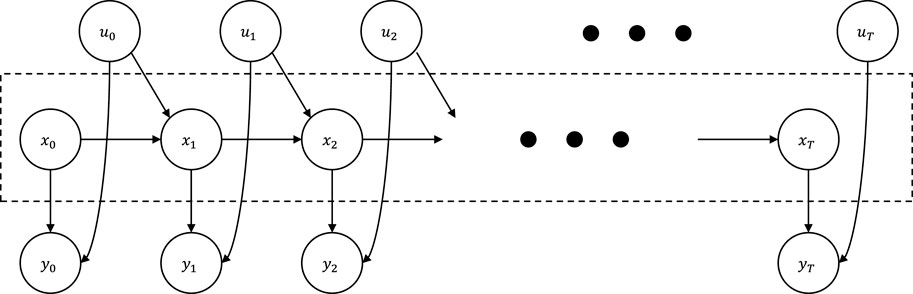
FIGURE 1. Probabilistic graphical model for stochastic dynamical systems with hidden states x_t, inputs u_t, and observations y_t.

The information on f(⋅), g(⋅), r(w), and q(v) is unavailable. In this study, the available information is the dataset U_T = {u₀, u₁, …, u_T} of system inputs and the dataset Y_T = {y₀, y₁, …, y_T} of observations. We want to learn models $\tilde{f}(\cdot )$, $\tilde{g}(\cdot )$, $\tilde{r}(w)$, and $\tilde{q}(v)$. The traditional view is to learn $\tilde{f}(\cdot )$, $\tilde{g}(\cdot )$, $\tilde{r}(w)$, and $\tilde{q}(v)$ for the sake of improving the performance of the root mean square (RMS) of predictions or maximizing the likelihood of the dataset. In this paper, we obtain a novel prediction model that gives a predictive interval of the observation. We define an interval of y_t as follows.

Definition 1. Let ${\mathcal{F}}_Y$ be the Borel set of ${\mathbb{R}}^d$. An interval $I_t\in {\mathcal{F}}_Y$ is a set of y_t. For a given probability level α ∈ (0, 1), if $I_t\in {\mathcal{F}}_Y$ satisfies

${\mathrm{P}\mathrm{r}}_t\left\{y_t\in I_t\in {\mathcal{F}}_Y\right\}\ge 1-\alpha ,(3)$

where ${\mathrm{P}\mathrm{r}}_t\{\cdot \}$ is the underlying probability measure defined on ${\mathcal{F}}_Y$ at time index t, we call I_t as a α-reliable interval. The set of all α − confidence intervals is defined as ${\mathcal{I}}_{t,\alpha }$. For a given probability level α ∈ (0, 1), an optimal interval $I_t^{*}$ satisfies

$\mathbb{C}\left(I_t^{*}\right)\le \mathbb{C}\left(I_t\right),\forall I_t\in {\mathcal{I}}_{\alpha },(4)$

where $\mathbb{C}(\cdot )$ denotes the capacity of a set.

The problem is formally summarized in Problem 1.

Problem 1. Given the system input set U_T = {u₀, u₁, …, u_T} and observation set U_T = {y₀, y₁, …, y_T}, to obtain ${\tilde{f}}^{*}(\cdot )$, ${\tilde{g}}^{*}(\cdot )$, ${\tilde{r}}^{*}(w)$, and ${\tilde{q}}^{*}(v)$ by solving

$\begin{array}{ll}\hfill & \underset{\tilde{f},\tilde{g},\tilde{r},\tilde{q}}{\min }\mathbb{C}\left(I_t\left(\tilde{f},\tilde{g},\tilde{r},\tilde{q}\right)\right)\hfill \\ \hfill & {\mathrm{P}\mathrm{r}}_t\left\{y_t\in I_t\left(\tilde{f},\tilde{g},\tilde{r},\tilde{q}\right)\in {\mathcal{F}}_Y\right\}\ge 1-\alpha ,\forall t=1,\dots ,T.\hfill \end{array}(5)$

3 Proposed method

In this section, we briefly review the reservoir computing and scenario approach. Then, we give the concept of interval reservoir computing, combining reservoir computing and a scenario approach. The probabilistic reliability of interval reservoir computing to Problem 1 is also given.

3.1 Brief introduction to reservoir computing

Reservoir computing is a novel algorithm to train a RNN. This study uses the echo state network (ESN) method presented in Jaeger and Haas (2004) to construct RNN. Let $x_{\mathrm{act},t}$ be the activation state of RNN at time index t. The terminology “echo” implies that $x_{\mathrm{act},t}$ is a function of all the input history u_t−1, … related to the network. The ESN consists of multiple sigmoidal units in discrete time, the so-called reservoir or dynamic reservoir. A general ESN has a discrete-time neural network with internal network units (for state $x_{\mathrm{sta},t}$), input units (for input u_t), and output units (for observation y_t). The internal units are updated as follows.

$x_{\mathrm{act},t+1}=f_{\mathrm{act}}\left(W^{\mathrm{in}}{u}_t+W{x}_{\mathrm{act},t}+W^{\mathrm{back}}{y}_t\right),(6)$

where $f_{\mathrm{act}}$ is the vector function of the internal unit written as $f_{\mathrm{act}}={\left[f_{\mathrm{act}}^1,\dots ,f_{\mathrm{act}}^{n_{\mathrm{act}}}\right]}^{\top }$.

On the other hand, the output is computed as

$y_t=W^{\mathrm{out}}{x}_{\mathrm{act},t},(7)$

where $W^{\mathrm{out}}$ is the output weight. Reservoir computing is to train $W^{\mathrm{in}}$, W, $W^{\mathrm{back}}$, and $W^{\mathrm{out}}$, and the algorithm is summarized as follows:

• Design of a reservoir vector: a reservoir vector $x_{\mathrm{act},t}$ and the internal unit, as shown in Eq. 6, are established.

• Randomly generating $W^{\mathrm{in}}$, W, and $W^{\mathrm{back}}$, which comprise a sparse random matrix with the maximal eigenvalue controlled.

• Determining the output layer by

$\underset{W^{\mathrm{out}}}{\min }{\displaystyle \sum _{t=1}^T}\Vert W^{\mathrm{out}}{x}_t-y_t{\Vert }^2+\beta \mathrm{T}\mathrm{r}\mathrm{a}\mathrm{c}\mathrm{e}\left(W^{\mathrm{out}}{W}^{\mathrm{out},\top }\right).(8)$

Figure 2 illustrates the reservoir computing concept.

FIGURE 2

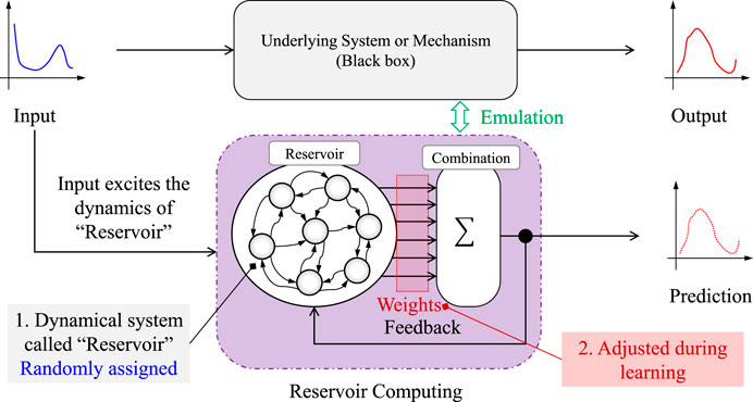
FIGURE 2. Intuitive introduction for reservoir computing.

3.2 Scenario approach

The scenario approach has been applied to obtain the probabilistic boundary for a given nonlinear state space model (Shen et al., 2020a). The theory of the scenario approach has been presented in Calafiore and Campi (2005) for solving robust optimization with the convex objective function and constraint functions. The result has been extended to non-convex cases in Campi et al. (2015). This paper reviews the method of Campi et al. (2015).

The decision variable is $\theta \in \mathrm{\Theta }\subseteq {\mathbb{R}}^{n_{\theta }}$. Let $J:\mathrm{\Theta }\to \mathbb{R}$ be the objective function. The uncertain variable is denoted by $\delta \in \mathrm{\Delta }\subseteq {\mathbb{R}}^{n_{\delta }}$. For every instance δ ∈ Δ, a subset of Θ is defined by

${\mathrm{\Theta }}_{\delta }=\left\{\theta \in \mathrm{\Theta }:h\left(\theta ,\delta \right)\le 0\right\},$

where $h:\mathrm{\Theta }\times \mathrm{\Delta }\to {\mathbb{R}}^m$ is a constraint function. Then, a robust optimization problem can be written as

$\begin{array}{cc}\hfill & \underset{\theta \in \mathrm{\Theta }}{\mathrm{m}\mathrm{i}\mathrm{n}}J\left(\theta \right)\hfill \\ \hfill & s.t.\theta \in {\mathrm{\Theta }}_{\delta },\forall \delta \in \mathrm{\Delta }.\hfill \end{array}(9)$

Problem Eq. 9 is NP-hard and cannot be solved by any algorithms for a general optimization problem. An approximate problem of that in Eq. 9 is obtained by sampling a dataset δ⁽¹⁾, …, δ^(N), which is written by

$\begin{array}{cc}\hfill & \underset{\theta \in \mathrm{\Theta }}{\mathrm{m}\mathrm{i}\mathrm{n}}J\left(\theta \right)\hfill \\ \hfill & s.t.\theta \in {\mathrm{\Theta }}_{{\delta }^{\left(i\right)}},\forall i=1,\dots ,N.\hfill \end{array}(10)$

Let ${\theta }_N^{*}$ be an optimal solution of the problem in Eq. 10 and ${\mathcal{A}}_N$ be an algorithm that is able to get ${\theta }_N^{*}$ for a given dataset (δ⁽¹⁾, …, δ^(N)) ∈ Δ^N. Then, we have

${\theta }_N^{*}={\mathcal{A}}_N\left({\delta }^{\left(1\right)},\dots ,{\delta }^{\left(N\right)}\right).(11)$

It is natural to doubt whether ${\theta }_N^{*}$ is a feasible solution of the problem in Eq. 9 since ${\theta }_N^{*}$ does not consider constraints for all δ ∈ Δ. Here, since the sampling process of the dataset (δ⁽¹⁾, …, δ^(N)) ∈ Δ^N is random, we consider the feasibility of ${\theta }_N^{*}$ in a probabilistic sense. We define the violation probability herein.

Definition 2. The violation probability of any decision θ ∈ Θ is written as

$\mathbb{V}\left(\theta \right)≔{\mathrm{P}\mathrm{r}}_{\delta }\left\{\delta \in \mathrm{\Delta }:\theta \notin {\mathrm{\Theta }}_{\delta }\right\},$

where ${\mathrm{P}\mathrm{r}}_{\delta }\{\cdot \}$ defines the probability measure defined on the σ-algebra of Δ.

For a given probability level ɛ ∈ (0, 1) and a given confidence bound 1 − β ∈ (0, 1), we want to get a bound of sample number $\bar{N}(\beta ,\epsilon )$ such that

${\mathrm{P}\mathrm{r}}_{\delta }\left\{\mathbb{V}\left({\theta }_N^{*}\right)\le \epsilon \right\}\ge 1-\beta ,\forall N\ge \bar{N}\left(\beta ,\epsilon \right).$

Theorem 1 of Campi et al. (2015) is stated as follows:

Lemma 1. Let ɛ : {0, …, N} → [0, 1] be a function such that

$\epsilon \left(N\right)=1(12)$

and

${\displaystyle \sum _{i=0}^{N-1}}\left(\genfrac{}{}{0pt}{}{N}{i}\right){\left(1-\epsilon \left(i\right)\right)}^{N-i}=\beta .(13)$

It holds that

${\mathrm{P}\mathrm{r}}^N\left\{\mathbb{V}\left({\theta }_N^{*}\right)>\epsilon \left(m_N^{*}\right)\right\}\le \beta ,(14)$

where $m_N^{*}$ is the number of irreducible subsamples of (δ⁽¹⁾, …, δ^(N)).

3.3 Interval reservoir computing

In this study, compared to obtain $W^{\mathrm{out}}$ by solving Eq. 8, we intend to find an interval of $W^{\mathrm{out}}$ for every given u_t, $x_{\mathrm{act},t}$ that can finally give an α-confident interval of y_t, as defined in Definition 1. In other words, the output will locate in an interval with a probability larger than the given level α ∈ (0, 1). In addition, the interval is expected to be optimal with the smallest area. Here, a sub-optimal interval is targeted as the approximation of $I_t^{*}$. For RNN, the interval is written as

$I_{\mathrm{RNN}}≔\left\{y=W^{\mathrm{Out}}{x}_{\mathrm{act},t}+e,W^{\mathrm{out}}\in \mathcal{W}\subseteq {\mathbb{R}}^{d\times n_{\mathrm{act}}},|e|\le \gamma \in {\mathbb{R}}^{+}\right\}.(15)$

Note that the set $I_{\mathrm{RNN}}$ is obtained by varying the values of $W^{\mathrm{out}}$, e in $\mathcal{W},$ and ${\mathbb{R}}^{+}$. A possible choice for the set Ω is a ball with center c and radius r > 0:

$\mathrm{\Omega }={\mathcal{B}}_{c,r}=\left\{W^{\mathrm{out}}\in \mathcal{W}:\Vert \omega -c{\Vert }_2\le r\right\}.(16)$

The interval output of the RNN obtained via Eq. 15 is explicitly written as

$\begin{array}{ll}\hfill I_{\mathrm{RNN},{\mathcal{B}}_{c,r}}\left(x_{\mathrm{act},t},\gamma \right)& =\left[c{x}_{\mathrm{act},t}-\left(r\Vert x_{\mathrm{act},t}\Vert +\gamma \right),c_{\mathrm{act},t}\right.+\left.\left(r\Vert x_{\mathrm{act},t}\Vert +\gamma \right)\right].\hfill \end{array}(17)$

Then, the problem of obtaining a spherical INN is written as

$\begin{array}{cc}\hfill & \underset{c,r,\gamma }{\mathrm{m}\mathrm{i}\mathrm{n}}\eta r+\gamma \hfill \\ \hfill & s.t.r,\gamma >0,\hfill \\ \hfill & \mathrm{P}\mathrm{r}\left\{y_t\in I_{\mathrm{RNN},{\mathcal{B}}_{c,r}}\left(x_{\mathrm{act},t},\gamma \right),\forall t\right\}\ge 1-\alpha ,\left({\mathcal{P}}_{\mathrm{B},\alpha }\right)\hfill \\ \hfill & y_t\in {\mathbb{R}}^d,\hfill \end{array}$

where η is a positive number. Let ${\theta }_{\mathrm{B}}$ be the decision variable of Problem ${\mathcal{P}}_{\mathrm{B},\alpha }$ including c, r, and γ. Let ${\mathrm{\Theta }}_{\mathrm{B},\alpha }$ be the feasible region of ${\theta }_{\mathrm{B}}$ of Problem ${\mathcal{P}}_{\mathrm{B},\alpha }$. Defining the optimal objective function of Problem ${\mathcal{P}}_{\mathrm{B},\alpha }$ by

$J_{\mathrm{B},\alpha }^{*}≔\underset{{\theta }_{\mathrm{B}}\in {\mathrm{\Theta }}_{\mathrm{B},\alpha }}{\min }\eta r+\gamma .(18)$

Defining the optimal solution set of Problem ${\mathcal{P}}_{\mathrm{B},\alpha }$ by

${\mathcal{A}}_{\mathrm{B},\alpha }^{*}≔\left\{{\theta }_{\mathrm{B}}\in {\mathrm{\Theta }}_{\mathrm{B},\alpha }:\eta r+\gamma =J_{\mathrm{B},\alpha }^{*}.\right\}.(19)$

Suppose that the dataset ${\mathcal{D}}_T={\{u(t),y(t)\}}_{t=1,\dots ,T}$ is available. Then, we can formulate the scenario program of Problem ${\mathcal{P}}_{\mathrm{B},\alpha }$ as follows:

$\begin{array}{cc}\hfill & \underset{c,r,\gamma }{\mathrm{m}\mathrm{i}\mathrm{n}}\eta r+\gamma \hfill \\ \hfill & s.t.r,\gamma >0,\hfill \\ \hfill & y_t\in I_{\mathrm{RNN},{\mathcal{B}}_{c,r}}\left(x_{\mathrm{act},t},\gamma \right),\forall t=1,\dots ,T.\left({˜\mathcal{P}}_{\mathrm{B},\alpha }^T\right)\hfill \end{array}$

Let ${\tilde{\mathrm{\Theta }}}_{\mathrm{B},\alpha }^T$ be the feasible region of ${\theta }_{\mathrm{B}}$ of Problem ${\tilde{\mathcal{P}}}_{\mathrm{B},\alpha }^T$. Defining the optimal objective function of Problem ${\tilde{\mathcal{P}}}_{\mathrm{B},\alpha }^T$ by

${\tilde{J}}_{\mathrm{B},\alpha }^T≔\underset{{\theta }_{\mathrm{B}}\in {\tilde{\mathrm{\Theta }}}_{\mathrm{B},\alpha }^T}{\min }\eta r+\gamma .(20)$

Defining the optimal solution set of Problem ${\tilde{\mathcal{P}}}_{\mathrm{B},\alpha }^T$ by

${\tilde{\mathcal{A}}}_{\mathrm{B},\alpha }^T≔\left\{{\theta }_{\mathrm{B}}\in {\tilde{\mathrm{\Theta }}}_{\mathrm{B},\alpha }^T:\eta r+\gamma ={\tilde{J}}_{\mathrm{B},\alpha }^T.\right\}.(21)$

By adapting Lemma 1, we have the following theorem on the probabilistic feasibility of ${\tilde{\theta }}_{\mathrm{B},\alpha }^T\in {\tilde{\mathcal{A}}}_{\mathrm{B},\alpha }^T$.

Theorem 1. Let ${\tilde{\theta }}_{\mathrm{B},\alpha }^T\in {\tilde{\mathcal{A}}}_{\mathrm{B},\alpha }^T$ be the solution of ${\tilde{\mathcal{P}}}_{\mathrm{B},\alpha }^T$. The interval at t associated with ${\tilde{\theta }}_{\mathrm{B},\alpha }^T$ is denoted by ${\tilde{I}}_{\mathrm{RNN},{\mathcal{B}}_{c,r}}^{\alpha }(x_{\mathrm{act},t},\gamma )$. Then, the following holds:

${\mathrm{P}\mathrm{r}}^T\left\{\mathrm{P}\mathrm{r}\left\{y_t\notin {\tilde{I}}_{\mathrm{RNN},{\mathcal{B}}_{c,r}}^{\alpha }\left(x_{\mathrm{act},t},\gamma \right)\right\}>\epsilon \left(m_T^{*}\right)\right\}\le \beta ,\forall t,(22)$

where $m_T^{*}$ is the number of irreducible subsamples of $\left((u_1,y_1),\dots ,(u_T,y_T)\right)$ and ɛ satisfies

$\epsilon \left(T\right)=1(23)$

and

${\displaystyle \sum _{i=0}^{T-1}}\left(\genfrac{}{}{0pt}{}{T}{i}\right){\left(1-\epsilon \left(i\right)\right)}^{T-i}=\beta .(24)$

Proof. Since ${\tilde{\theta }}_{\mathrm{B},\alpha }^T$ is a feasible solution of ${\tilde{\mathcal{P}}}_{\mathrm{B},\alpha }^T$, by Lemma 1, we have

${\mathrm{P}\mathrm{r}}^T\left\{\mathbb{V}\left({\tilde{\theta }}_{\mathrm{B},\alpha }^T\right)>\epsilon \left(m_T^{*}\right)\right\}\le \beta ,(25)$

where $\mathbb{V}({\tilde{\theta }}_{\mathrm{B},\alpha }^T)=\mathrm{P}\mathrm{r}\left\{y_t\notin {\tilde{I}}_{\mathrm{RNN},{\mathcal{B}}_{c,r}}^{\alpha }(x_{\mathrm{act},t},\gamma )\right\}$. Thus, Eq. 22 holds.

By Theorem 1, we know that it can adjust the sample number T to regulate the violation probability. Using the scenario approach directly, it cannot regulate the violation probability to the desired one. We leave this issue for future work. Based on the theoretical analysis, the algorithm for interval reservoir computing is designed, and the pseudo-code is written in Algorithm 1.

Algorithm 1.Algorithm for interval reservoir computing.

 Inputs: data set ${\mathcal{D}}_T={\{u(t),y(t)\}}_{t=1,\dots ,T}$

  1: design of reservoir vector and function according to Eqs 6, 7

  2: randomly generate $W^{\mathrm{in}}$, W, and $W^{\mathrm{back}}$

  3: solve Problem ${\tilde{\mathcal{P}}}_{\mathrm{B},\alpha }^T$ and obtain ${\tilde{\theta }}_{\mathrm{B},\alpha }^T$

 Output: ${\tilde{\theta }}_{\mathrm{B},\alpha }^T$

Figure 3 illustrates the proposed framework for implementing the interval reservoir computing method. It follows the general framework widely used to validate the time series model (Shen et al., 2020b). The online obtained history data range from the blue line (not the whole line). Then, the data are used to give the future maximum likelihood prediction (the red dotted line) and the confidence region (the red line) by the model trained by the training dataset.

FIGURE 3

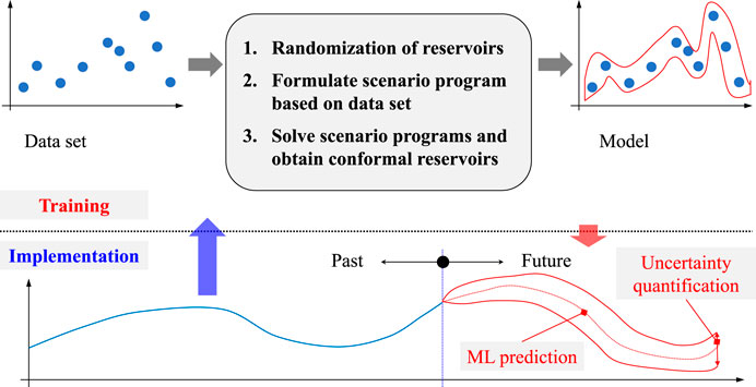
FIGURE 3. Proposed framework of the interval reservoir computing method.

4 Validations

4.1 Wind power prediction

Let $x_{\mathrm{s}}(t)$ be the wind speed at time index t and $y_{\mathrm{p}}(t)$ be the wind power at time index t. The mechanism behind the evolution of wind speed and wind power can be described by

$x_{\mathrm{s}}\left(t+1\right)=f_{\mathrm{wind}}\left(x_{\mathrm{s}}\left(t\right),w_{\mathrm{s}}\left(t\right)\right),(26)$

$y_{\mathrm{p}}\left(t\right)=g_{\mathrm{wind}}\left(x_{\mathrm{s}}\left(t\right),v_{\mathrm{s}}\left(t\right)\right).(27)$

Here, both $f_{\mathrm{wind}}$ and $g_{\mathrm{wind}}$ are unknown.

The experimental dataset shown in Figure 4 is used in this validation. Figure 4A plots the time series data on wind speed, and Figure 4B plots the time series data on the wind power at the same time. There are a total of 13 groups of data. Eight groups are used as training datasets; the other groups are used as test datasets.

FIGURE 4

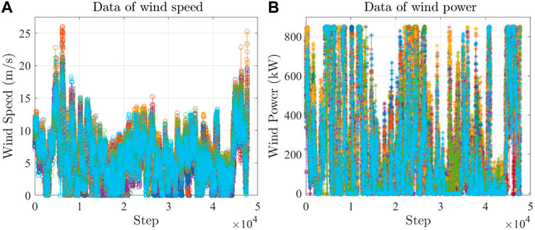
FIGURE 4. Experimental dataset in this study.

In this validation, we set the threshold for violation probability as α = 0.05. The number of samples, N, is from {100, 500, 1000, 2000, 5000, 10,000}. Figures 5, 6 show two examples of the one-step-ahead prediction by the proposed interval reservoir computing. The parts (a), (b), (c), and (d) of each figure provide the results with N = 500, N = 1000, N = 2000, and N = 5000, respectively. As the sample number N increases, the size of the interval also increases, while the center of the interval does not change significantly. In particular, as N surpluses 2,000, the probability of having the data inside the interval is less than the required value α = 0.05, implying that the proposed method gives a more conservative interval than we expect.

FIGURE 5

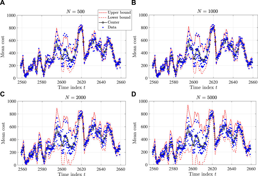
FIGURE 5. Results of a one-step-ahead prediction by the proposed interval reservoir computing (from t = 2560 to t = 2660): (A) N = 500, (B) N = 1000, (C) N = 2000, and (D) N =5000.

FIGURE 6

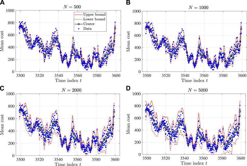
FIGURE 6. Results of a one-step-ahead prediction by the proposed interval reservoir computing (from t = 2560 to t = 2660): (A) N = 500, (B) N = 1000, (C) N = 2000, and (D) N = 5000.

A statistical analysis has been conducted to check the performance of the proposed interval reservoir computing. Monte Carlo tests have been repeated 5,000 times for each choice of sample number N = 100, 500, 1000, 2000, 5000, 10,000. We check the violation probability and CPU time in this Monte Carlo simulation. The metric for checking the performance of the violation probability is ${\mathrm{P}\mathrm{r}}^N\{\mathbb{V}({\theta }_N^{*})>0.05\}$, the chance that the violation probability is larger than 0.05. As N increases, ${\mathrm{P}\mathrm{r}}^N\{\mathbb{V}({\theta }_N^{*})>0.05\}$ decreases to zero quickly, as shown in Table 1. On the other hand, the computation time increases as N increases while it is still at an acceptable level.

TABLE 1

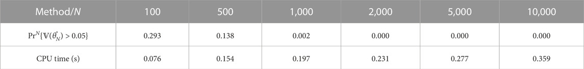
TABLE 1. Statistical performance of the proposed method with different sample numbers N. Mean values of 5,000 Monte Carlo trials are presented.

4.2 Vehicle trajectory prediction

In another example, we have applied the proposed interval reservoir computing to vehicle trajectory prediction. The experimental data are the public dataset “US Highway 101 Dataset.” As in the example of wind power prediction, the number of samples is chosen from {100, 500, 1000, 2000, 5000, 10,000}, and the violation probability threshold is α = 0.05. Figure 7 shows one example of a one-step-ahead prediction for the vehicle trajectory prediction with N = 500 and N = 5000 results.

FIGURE 7

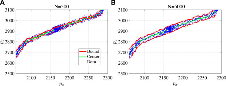
FIGURE 7. One example of a one-step-ahead prediction by the proposed interval reservoir computing for vehicle trajectory prediction: (A) N = 500 and (B) N = 5000.

Statistical analysis has also been conducted in this example of vehicle trajectory prediction. The settings of Monte Carlo tests are the same as the example of wind power prediction. As shown in Table 2, the results are consistent with the results of wind power prediction.

TABLE 2

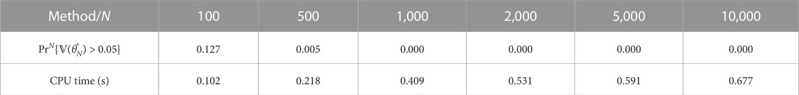
TABLE 2. Statistical performance of the proposed method with different sample numbers N. Mean values of 5,000 Monte Carlo trials are presented.

4.3 Discussion

In this validation, we mainly check the performance of the proposed method with different sample numbers. Indeed, it is necessary to compare the proposed method with other uncertainty quantification methods, such as conformal prediction and Bayesian neural networks. We will further research on this as future work.

One drawback of the proposed interval reservoir computing is that it cannot give an exact interval for a given violation probability α. This drawback comes from using a scenario approach to solve the problem ${\mathcal{P}}_{B,\alpha }$. The scenario approach ensures the approximate solution’s feasibility while not considering the convergence of the approximate solution’s optimality. Using sample discarding presented in (Campi and Garatti, 2011) seems to be an excellent choice to make a trade-off between optimality and feasibility. However, sample discarding will dramatically increase the computational complexity of solving ${\mathcal{P}}_{B,\alpha }$. We leave the issue of optimality for future work.

5 Conclusion and future work

This paper proposes an improved version of interval reservoir computing for time series data forecasting, for example, wind power forecasting and vehicle trajectory forecasting. More than giving a maximum likelihood prediction value of wind power or vehicle trajectory, interval reservoir computing provides an interval of the prediction. The future data will be located inside the interval with a probability larger than the required value. To obtain the interval, a chance-constrained optimization has to be solved for obtaining the interval of the parameters in an RNN. We apply a scenario approach to solve the chance-constrained optimization problem. Experimental data-based validations have been conducted to evaluate the proposed interval reservoir computing. Although the results show that the proposed interval reservoir computing can give a tight interval for wind power forecasting and vehicle trajectory forecasting, the following issues remain to be resolved in future work.

• It is necessary to compare the proposed method with other uncertainty quantification methods, such as the conformal prediction and Bayesian neural networks.

• The scenario approach for solving chance-constrained optimization cannot ensure the convergence of the optimality of the approximate solution. Thus, it is necessary to develop a method that ensures the convergence of the optimality to solve the chance-constrained optimization.

Data availability statement

The original contributions presented in the study are included in the article/Supplementary material; further inquiries can be directed to the corresponding author.

Author contributions

L-DG: methodology, software, validation, formal analysis, data curation, writing–original draft, and writing–review and editing. Z-HL: conceptualization, methodology, writing–original draft, writing–review and editing, supervision, and funding acquisition. M-YW: conceptualization, methodology, writing–original draft, and writing–review and editing. Q-LF: methodology, writing–original draft, and writing–review and editing. LX: data curation. Z-MZ: data curation. Y-YL: data curation. Y-PZ: supervision and funding acquisition. All authors contributed to the article and approved the submitted version.

Acknowledgments

This work is supported by the Opening Project of Key Laboratory of Technology on Intelligent Transportation Systems, Ministry of Transport, Beijing, China.

Conflict of interest

The authors declare that the research was conducted in the absence of any commercial or financial relationships that could be construed as a potential conflict of interest.

Publisher’s note

All claims expressed in this article are solely those of the authors and do not necessarily represent those of their affiliated organizations, or those of the publisher, the editors, and the reviewers. Any product that may be evaluated in this article, or claim that may be made by its manufacturer, is not guaranteed or endorsed by the publisher.

References

Ak, R., Vitelli, V., and Zio, E. (2015). An interval-valued neural network approach for uncertainty quantification in short-term wind speed prediction. IEEE Trans. Neural Netw. Learn. Syst. 26, 2787–2800. doi:10.1109/tnnls.2015.2396933

PubMed Abstract | CrossRef Full Text | Google Scholar

Calafiore, G., and Campi, M. C. (2005). Uncertain convex programs: randomized solutions and confidence levels. Math. Program. 102, 25–46. doi:10.1007/s10107-003-0499-y

CrossRef Full Text | Google Scholar

Campi, M., and Garatti, S. (2011). A sampling-and-discarding approach to chance-constrained optimization: feasibility and optimality. J. Optim. Theory Appl. 148, 257–280. doi:10.1007/s10957-010-9754-6

CrossRef Full Text | Google Scholar

Campi, M., Garatti, S., and Ramponi, F. (2015). A general scenario theory for nonconvex optimization and decision making. IEEE Trans. Automatic Control 63, 4067–4078. doi:10.1109/tac.2018.2808446

CrossRef Full Text | Google Scholar

Campi, M. C., Calafiore, G., and Garatti, S. (2009). Interval predictor models: identification and reliability. Automatica 45, 382–392. doi:10.1016/j.automatica.2008.09.004

CrossRef Full Text | Google Scholar

Chen, C., Lu, C., Wang, B., Trigoni, N., and Markham, A. (2021). Dynanet: neural kalman dynamical model for motion estimation and prediction. IEEE Trans. Neural Netw. Learn. Syst. 32, 5479–5491. doi:10.1109/tnnls.2021.3112460

PubMed Abstract | CrossRef Full Text | Google Scholar

Chen, Z., Wu, L., and Shahidehpour, M. (2015). Effective load carrying capability evaluation of renewable energy via stochastic long-term hourly based scuc. IEEE Trans. Sustain. Energy 6, 188–197. doi:10.1109/tste.2014.2362291

CrossRef Full Text | Google Scholar

Dai, C., Wu, L., and Wu, H. (2016). A multi-band uncertainty set based robust scuc with spatial and temporal budget constraints. IEEE Trans. Power Syst. 31, 4988–5000. doi:10.1109/tpwrs.2016.2525009

CrossRef Full Text | Google Scholar

Evans, M., Bono, C., and Wang, Y. (2021). Toward net-zero electricity in europe: what are the challenges for the power system? IEEE Power Energy Mag. 20, 44–54. doi:10.1109/mpe.2022.3167575

CrossRef Full Text | Google Scholar

Garattia, S., Campib, M., and Care, A. (2019). On a class of interval predictor models with universal reliability. Automatica 110, 108542. doi:10.1016/j.automatica.2019.108542

CrossRef Full Text | Google Scholar

Ge, X., Qian, J., Fu, Y., Lee, W., and Mi, Y. (2022). Transient stability evaluation criterion of multi-wind farms integrated power system. IEEE Trans. Power Syst. 37, 3137–3140. doi:10.1109/tpwrs.2022.3156430

CrossRef Full Text | Google Scholar

Hu, B., and Wu, L. (2016). Robust scuc with multi-band nodal load uncertainty set. IEEE Trans. Power Syst. 31, 2491–2492. doi:10.1109/tpwrs.2015.2449764

CrossRef Full Text | Google Scholar

Hu, B., Wu, L., and Marwali, M. (2014). On the robust solution to scuc with load and wind uncertainty correlations. IEEE Trans. Power Syst. 29, 2952–2964. doi:10.1109/tpwrs.2014.2308637

CrossRef Full Text | Google Scholar

Ishibuki, H., Tanaka, H., and Okada, H. (1993). An architecture of neural networks with interval weights and its application to fuzzy regression analysis. Fuzzy Sets Syst. 57, 27–39. doi:10.1016/0165-0114(93)90118-2

CrossRef Full Text | Google Scholar

Jaeger, H., and Haas, H. (2004). Harnessing nonlinearity: predicting chaotic systems and saving energy in wireless communication. Science 304, 78–80. doi:10.1126/science.1091277

PubMed Abstract | CrossRef Full Text | Google Scholar

Liu, H., Flores, C. E., Spring, J., Shladover, S. E., and Lu, X. Y. (2022a). Field assessment of intersection performance enhanced by traffic signal optimization and vehicle trajectory planning. IEEE Trans. Intelligent Transp. Syst. 23, 11549–11561. doi:10.1109/tits.2021.3105329

CrossRef Full Text | Google Scholar

Liu, Y., Zhou, B., Wang, X., Li, L., Cheng, S., Chen, Z., et al. (2022b). Dynamic lane-changing trajectory planning for autonomous vehicles based on discrete global trajectory. IEEE Trans. Intelligent Transp. Syst. 23, 8513–8527. doi:10.1109/tits.2021.3083541

CrossRef Full Text | Google Scholar

Lyu, N., Wen, J., Duan, Z., and Wu, C. (2022). Vehicle trajectory prediction and cut-in collision warning model in a connected vehicle environment. IEEE Trans. Intelligent Transp. Syst. 23, 966–981. doi:10.1109/tits.2020.3019050

CrossRef Full Text | Google Scholar

Neal, R. (2012). Bayesian learning for neural networks, 118. Springer Science and Business Media.

Google Scholar

Shen, X., Ouyang, T., Yang, N., and Zhuang, J. (2023). Sample-based neural approximation approach for probabilistic constrained programs. IEEE Trans. Neural Netw. Learn. Syst. 34, 1058–1065. doi:10.1109/tnnls.2021.3102323

PubMed Abstract | CrossRef Full Text | Google Scholar

Shen, X., Ouyang, T., Zhang, Y., and Zhang, X. (2020a). Computing probabilistic bounds on state trajectories for uncertain systems. IEEE Trans. Emerg. Top. Comput. Intell. early access 7, 285–290. doi:10.1109/TETCI.2020.3019040

CrossRef Full Text | Google Scholar

Shen, X., and Raksincharoensak, R. (2022). Pedestrian-aware statistical risk assessment. IEEE Trans. Intelligent Transp. Syst. 23, 7910–7918. doi:10.1109/tits.2021.3074522

CrossRef Full Text | Google Scholar

Shen, X., Zhang, Y., Sata, K., and Shen, T. (2020b). Gaussian mixture model clustering-based knock threshold learning in automotive engines. IEEE/ASME Trans. Mechatronics 25, 2981–2991. doi:10.1109/tmech.2020.3000732

CrossRef Full Text | Google Scholar

Wang, P., Wang, P., Wang, D., and Xue, B. (2021). A conformal regressor with random forests for tropical cyclone intensity estimation. IEEE Trans. Geoscience Remote Sens. 60, 1–14. doi:10.1109/tgrs.2021.3139930

CrossRef Full Text | Google Scholar

Wen, H., Gu, J., Ma, J., Yuan, L., and Jin, Z. (2021). Probabilistic load forecasting via neural basis expansion model based prediction intervals. IEEE Trans. Smart Grid 12, 3648–3660. doi:10.1109/tsg.2021.3066567

CrossRef Full Text | Google Scholar

Xue, B., Hu, S., Xu, J., Geng, M., Liu, X., and Meng, H. (2022). Bayesian neural network language modeling for speech recognition. IEEE/ACM Trans. Audio, Speech, Lang. Process. 30, 2900–2917. doi:10.1109/taslp.2022.3203891

CrossRef Full Text | Google Scholar

Yu, Y., Shan, D., Benderius, O., Berger, C., and Kang, Y. (2022). Formally robust and safe trajectory planning and tracking for autonomous vehicles. IEEE Trans. Intelligent Transp. Syst. 23, 22971–22987. doi:10.1109/tits.2022.3196623

CrossRef Full Text | Google Scholar

Zhao, Y., Ye, L., Wang, W., Sun, H., Ju, Y., and Tang, Y. (2018). Data-driven correction approach to refine power curve of wind farm under wind curtailment. IEEE Trans. Sustain. Energy 9, 95–105. doi:10.1109/tste.2017.2717021

CrossRef Full Text | Google Scholar