Wind power output prediction in complex terrain based on modal decomposition attentional convolutional network

In this work, modal decomposition is employed to generate more data for matching scenarios with more complex topography for predicting wind power output in the case of complex terrain. The existing literature shows that a single wind power output forecast model is difficult to cope with complex terrain and thus the accuracy of wind power output forecast is limited. This work combines the advantages of attention mechanism and convolutional neural network for a novel network based on modal decomposition of historical data for wind power output forecast on complex terrain. The proposed novel network can break through the limitations of a single wind power output forecast model. In addition, the signals that are modally decomposed can be predicted more accurately. The presented method is contrasted with various other algorithms for the wind power output prediction problem in complex terrain. Comparative experiments show that the proposed network achieves a higher accuracy rate.

1 Introduction

Many countries worldwide have joined carbon neutral and carbon peaking programs to protect the environment and sustainable development (Ma et al., 2023). For example, China is speeding up the development of new electric power systems based on new sources of energy. While new energy sources bring environmental protection to the new power systems, new energy sources also bring challenges to the economic dispatch of the systems (Qi et al., 2023). For example, wind power output in complex terrain brings many burdens for dispatch of power systems (Wang et al., 2022). Fast, long-term and accurate forecasting of wind power output in complex terrain is an essential foundation for ensuring the secure and robust performance of new power systems (Qian and Ishihara, 2022).

Wind power output is affected by complex terrain and climate. The popular data-driven methods for predicting wind energy output fall into the following five categories: time series methods, deep neural network methods, convolutional neural network (CNN) methods, other single model regression methods, and combined data-driven methods (Chen et al., 2021).

The more representative time series methods are recurrent neural network (RNN) series methods and temporal convolutional network methods. Recurrent neural network methods have been gradually developed into long and short-term memory (LSTM) network method, bidirectional long and short-term memory (BiLSTM) network method, and gated recurrent unit (GRU) method (Shahid et al., 2020). The temporal convolutional network methods have been further developed as temporal convolutional network methods with multi-feature spatio-temporal fusion (GuZhaoJian, 2022). The time-series data-driven methods are suitable for cases with very small amounts of inputs and strong signal continuity (López-Oriona and Vilar, 2021). For example, RNNs are more accurate than historical averaging (HA), autoregressive integrated moving average model (ARIMA), and vector autoregressive model (VAR) methods in the field of predicting crowd flows (Tang et al., 2022). LSTM network method can be utilized for predicting the prices of some energy products, such as carbon and oil (Zhou et al., 2022). The BiLSTM network is more effective in predicting time series than the LSTM network (Kulshrestha et al., 2020). The GRU method is a time series method based on the LSTM network, and is theoretically more effective than the LSTM network for time series (Sun et al., 2023). Temporal convolutional networks have been utilized to predict the electricity load in multiple regions (Yin and Xie, 2021). The attentional mechanism approach has been combined with temporal convolutional networks to solve the remaining useful life (RUL) prediction problem (Wang et al., 2021).

Deep neural networks are most skilled in the characterization of multiple inputs and multiple outputs (Shi et al., 2020). Deep neural networks represented by deep fully connected layers have even been applied behind recurrent and CNNs to characterize the connection between input and output (Ashtiani et al., 2022). The use of deep neural networks alone to characterize multi-input and multi-output relationships has limitations as well (Yang et al., 2022). Combining LSTM and graph convolutional networks to form a two-channel deep network model results in superior results to the single-channel deep neural network approach, however, the accuracy still has room to rise. And the dual-channel deep network model is utilized for super-short-term forecasting and has some limitations (Liu et al., 2023).

Although the inputs of most convolutional neural networks are pictures, historical data and complex terrain data can be arranged in the form of pictures and entered into convolutional neural networks for predicting wind power output (Yildiz et al., 2021). Compared to time series or feature inputs, the information contained in the pictures that a convolutional neural network requires as input is enormous (Harbola and Coors, 2019). Convolutional neural networks, represented by residual networks, have been applied to wind power output prediction, obtaining more accurate results than other comparative algorithms (Yin and Liu, 2020).

Other single data-driven models for predicting wind energy output or load electricity utilization abound. For example, the deep forest regression algorithm has been employed for forecasting near-term loads (He et al., 2020). Multi-layer support vector machine regression model has been applied to prediction problems for obtaining accurate predictions (Lv et al., 2020). Adding potential random variables to the encoder-decoder network can accurately model complex wind speeds and wind sequences (Zheng and Zhang, 2023). The four single time series forecasting models mentioned above have different superiority in different problems, however, the four models all have some limitations (Lin et al., 2020).

To address the limitations of a single model, many combined data-driven methods have been presented to deal with problems like prediction or classification. For example, CNNs, deep neural networks, and LSTM networks were combined to solve image sequence prediction tasks (Balderas et al., 2019). LSTM networks were combined with autoencoder neural networks for solving the monitoring problem of inhomogeneous dynamic processes (Deng et al., 2023). CNNs and attention mechanisms (AM) were combined for forecasting wind speed, and utilizing ensemble empirical modal decomposition for removing noise from the raw wind speed data as well (Shang et al., 2023). Combining the modeling approach with the convolutional neural network approach, wind power time series expressed as ordinary differential equations are predicted with neural networks incorporating AM (Liu et al., 2022). Convolutional neural networks and sparse pooling layers are combined for extracting potential features describing local spatial correlations in the raw data and retaining meaningful values that have the highest probability of contributing to the final prediction. The underlying temporal characteristics of the output are fetched by the recursive process of LSTM (Liu and Zhang, 2022). K-shape and K-mean guided CNN combined with GRU for over prediction of wind turbine power production (Liu et al., 2021). Inspired by the above five data-driven methods, this work presents a modal decomposition attentional convolutional network (MDACN) based prediction method combining modal decomposition, attentional mechanism and convolutional neural network to tackle the wind power output forecasting issue in complex terrain. A summary of the contributions of this work is set out below:

(1) This work incorporates the modal decomposition method based on the state-of-the-art algorithm of the new energy output prediction. Modal decomposition removes noise from the raw data and refines the mixed features into distinct features to be predicted separately. The data-driven approach incorporating the modal decomposition is able to forecast wind energy output more accurately.

(2) In addition, this work incorporates an AM based on the latest new energy output prediction algorithm. The data-driven method incorporating AM that assign weights to different data can reduce the pressure on network processing, speed up network training, and reduce the dependence of the network on computational memory.

(3) The MDACN proposed in this work is based on the state-of-the-art BiLSTM network. The network proposed in this work overcomes the limitations of a single data-driven model and employs deep fully connected layers for overcoming the disadvantages of a single data-driven model with low accuracy.

The rest of the chapters in this article are arranged as follows. Section 2 of this work presents the issues and evaluation metrics associated with wind output model of complex terrain. Section 3 of this work presents the proposed MDACN method in detail. Section 4 of this work presents the specific experimental results. Section 5 of this work briefly summarizes the work.

2 Wind power output prediction model of complex terrain

2.1 Characteristics of wind power output prediction in complex terrain

Wind farms in complex terrain, such as mountain wind farms, are characterized by complex topography, large differences in wind elevation, significant differences in wind speed and wind direction, irregular tail currents, and different turbulence effects, these factors contribute to the difficulty of wind power prediction in wind farms in complex terrain. Hills, cliffs, steep slopes, and ridges all have additional effects on wind speed: peaks or mountain tops have an acceleration effect on the wind, and bottoms or valleys have a deceleration effect on the wind. Temperature, pressure, and air density are affected by changes in altitude. In high altitude areas, the unique conditions, such as high altitude, frequent thunderstorms, low wind density, low average wind speed, frequent wind direction changes, and complex terrain conditions in mountain wind farms, can result in more difficult wind power predictions.

2.2 Wind power output model of complex terrain

2.2.1 Statistical model

Statistical models, called time series models as well, are mainly based on historical wind measurement data and are built based on statistical methods of parameter estimation combined with pattern recognition. The most commonly applied statistical models are autoregressive models (AR), moving average models (MA), and autoregressive dynamic adaptive models (ARDA). The model is suitable for short-term (less than 6 hours) forecasting on small time scales.

2.2.2 Physical model

A typical physical model is numerical weather prediction. Numerical weather prediction is a method of calculating numerically by means of a mainframe machine on the basis of actual atmospheric conditions and under specified initial and marginal conditions. Then, predicting the state of atmospheric motion and weather phenomena for a future period by solving a system of equations characterizing the evolution of weather. This method is more suitable for medium-term (generally more than 6 hours) wind speed prediction.

2.2.3 Dynamic spatio-temporal model

Dynamic spatio-temporal model requires to consider the temporal sequences of wind velocities at the wind field and the surrounding wind measurement points, based on the correlation between the wind velocity of the surrounding wind measurement points and the wind farm for prediction. Generally, several remote monitoring points around the wind farm are required to forecast wind velocity and wind direction based on the correlation results, resulting in smaller errors, generally within a short period of time (one to 4 hours). In fact, the error is mainly related to the number of monitoring points in the wind farm.

2.2.4 Intelligent model of artificial neural network (ANN)

In contrast to statistical and physical models, intelligent model of ANN is data-driven and has machine learning capabilities. The intelligent model of ANN has the advantage of high precision by utilizing the method of fuzzy logic and vector machine learning theory, utilizing historical data, barometric pressure and temperature as inputs to build a prediction model for wind speed without establishing the atmospheric equations of motion.

2.2.5 Combined prediction model

Each forecasting model has theoretical limitations, and to optimize the forecasting process and provide forecasting accuracy, combined forecasting is increasingly applied in practice. For example, the optimized physical model and the artificial intelligence model combined with the dual model, exploiting various physical situations (e.g., wake effect) to simulate the atmospheric processes and obtain the physical model to obtain the wind velocity prediction. The wind velocity is considered as importation and the wind power output is predicted by intelligent models with neural networks, and the results obtained are more accurate than those of other models.

2.3 Evaluation index of wind power output model on complex terrain

To provide a more intuitive comparison of the accuracy of different prediction methods, six assessment metrics are cited.

Sum of squares for error (SSE) Eq. 1:

$\text{SSE}=\sum _{\mathrm{i}=1}^{\mathrm{n}}{\left({\mathrm{y}}_{\mathrm{i}}-{\widehat{\mathrm{y}}}_{\mathrm{i}}\right)}^2,(1)$

The scope of values is (0,+∞) and if the forecasted results match the real results, then the model is an ideal model. As the error increases, the value increases and the behavior of the model decreases.

Mean squared error (MSE) Eq. 2:

$\text{MSE}=\frac{1}{\mathrm{n}}\sum _{\mathrm{i}=1}^{\mathrm{n}}{\left({\mathrm{y}}_{\mathrm{i}}-{\widehat{\mathrm{y}}}_{\mathrm{i}}\right)}^2,(2)$

Root mean square error (RMSE) Eq. 3:

$\text{RMSE}=\sqrt{\frac{1}{\mathrm{n}}\sum _{\mathrm{i}=1}^{\mathrm{n}}{\left({\mathrm{y}}_{\mathrm{i}}-{\widehat{\mathrm{y}}}_{\mathrm{i}}\right)}^2},(3)$

Mean absolute error (MAE) Eq. 4:

$\text{MAE}=\frac{1}{\mathrm{n}}\sum _{\mathrm{i}=1}^{\mathrm{n}}\left|{\mathrm{y}}_{\mathrm{i}}-{\widehat{\mathrm{y}}}_{\mathrm{i}}\right|,(4)$

The MAE is the average of the extreme difference between the forecast and the actual value, and better reflects the reality of the forecast error. The scope of values is (0,+∞) and if the forecasted results match the real results, then the model is an ideal model. As the error increases, the value increases and the behavior of the model decreases.

Symmetric mean absolute percentage error (SMAPE) Eq. 5:

$\text{SMAPE}=\frac{100\%}{\mathrm{n}}\sum _{\mathrm{i}=1}^{\mathrm{n}}\frac{\left|{\mathrm{y}}_{\mathrm{i}}-{\widehat{\mathrm{y}}}_{\mathrm{i}}\right|}{\left(\left|{\widehat{\mathrm{y}}}_{\mathrm{i}}\right|+\left|{\mathrm{y}}_{\mathrm{i}}\right|\right)/2},(5)$

In the scope of [0,+∞], a SMAPE value of zero represents a performe model, whereas a SMAPE value higher than 100% represents a model of unfavorable quality.

Coefficient of determination (R2-R-Square) Eq. 6:

$\mathrm{R}2=1-\frac{\sum _{\mathrm{i}}{\left({\widehat{\mathrm{y}}}_{\mathrm{i}}-{\mathrm{y}}_{\mathrm{i}}\right)}^2}{\sum _{\mathrm{i}}{\left({\overline{\mathrm{y}}}_{\mathrm{i}}-{\mathrm{y}}_{\mathrm{i}}\right)}^2},(6)$

The R2 judgment factors are drawn from [0, 1]. when R2 = 1, it indicates that the model adequately forecasts the material; when the value of R2 is zero, it indicates that the model fails to provide a reasonable description of the material evolution. Generally, the R2 judgment factors are employed to measure the performance of each model, and when its number is approaching 1, it shows that the model is better able to interpret more changes in the data.

From the formula, $n$ is the count of forecast sites, $y_i$ and ${\widehat{y}}_i$ are the actual and forecast results in point $i$ of the data set, separately.

3 Modal decomposition attentional convolutional network

The proposed MDACN combines the advantages of modal decomposition, attention mechanism, and convolutional neural network. The steps of the MDACN are presented in Figure 1. The wind velocity and wind energy output data are first decomposed by CEEMDAN into modal components with more refined characteristics. Each modal component is weighted separately with the AM, giving higher weights to important data. The weighted data are then predicted by BiLSTM, and finally each modal component of the prediction is summed up to obtain the final result.

FIGURE 1

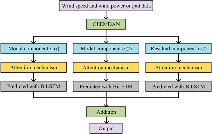
FIGURE 1. Steps of proposed MDACN.

3.1 Modal decomposition in proposed modal decomposition attentional convolutional network

Modal decomposition breaks down the raw signals into modal components with more regular characteristics. Features that are more distinct and easy to categorize are extracted for separate prediction, preventing low accuracy caused by feature mixing clutter. The pre-processing of the original data utilizing the method of mode decomposition results in better characterization, thus improving the reliability of the forecasts. This project intended to improve the accuracy of decomposition by capitalizing on the complete ensemble empirical mode decomposition with adaptive noise (CEEMDAM), which effectively overcomes the problems of mode aliasing and the presence of excess noise in the decomposed signal. The CEEMDAN process in MDACN (Figure 2) is as follows. First, white noise with different positive and negative components is added to the original signal $\mathrm{x}\left(\mathrm{t}\right)$ to obtain the new signal $\mathrm{x}\left(\mathrm{t}\right)\pm {\mathrm{n}}_{\mathrm{i}}\left(\mathrm{t}\right)$. On this basis, the empirical mode decomposition (EMD) method is adopted to acquire the first-order mode components ${\mathrm{c}}_{\mathrm{i},1+}\left(\mathrm{t}\right)$ and ${\mathrm{c}}_{\mathrm{i},1-}\left(\mathrm{t}\right)$ for every fresh signal. Then, the first-order vibrational components ${\mathrm{c}}_1\left(\mathrm{t}\right)$ are obtained by summing and averaging the first-order vibrational components, as Eq. 7

${\mathrm{c}}_1\left(\mathrm{t}\right)={\displaystyle \sum _{\mathrm{k}=1}^{\mathrm{i}}}\left({\mathrm{c}}_{\mathrm{k},1+}\left(\mathrm{t}\right)+{\mathrm{c}}_{\mathrm{k},1-}\left(\mathrm{t}\right)\right)(7)$

FIGURE 2

FIGURE 2. Steps of CEEMDAN in MDACN.

Subtracting the first-order vibrational components from the original input signal, the resulting first-order residual constituent is Eq. 8:

${\mathrm{x}}_2\left(\mathrm{t}\right)=\mathrm{x}\left(\mathrm{t}\right)-{\mathrm{c}}_1\left(\mathrm{t}\right)(8)$

White noise is appended to the input signal until a residual component is produced, the process is called S1. Next, each residual component is employed as an import signal until the output mode constituents ${\mathrm{c}}_1\left(\mathrm{t}\right)$, ${\mathrm{c}}_2\left(\mathrm{t}\right)$ and the residual constituent ${\mathrm{x}}_3\left(\mathrm{t}\right)$.

Through modal decomposition, the original signal is broken down into a series of modal components with different rules. These modal components contain more information and are easier to be classified and predicted. By extracting these regular features, the problem of low accuracy resulting from feature mixing and clutter can be effectively avoided.

3.2 Attention mechanism in proposed modal decomposition attentional convolutional network

The basic idea of the AM is to divide the raw data into an array of <Key,Value> couples. For a specific goal factor Query, the degree of resemblance or similarity with each keyword is compared, the weights of each keyword are calculated, and then a weighting operation is performed on each keyword to achieve the ultimate result. Then, based on the theory of fuzzy sets, the weights of each factor are calculated by adding up the weights of each factor, and then combining the Query and Key. If Value is denoted as ${\mathrm{L}}_{\mathrm{x}}$, the fundamental concept can be expressed as Eq. 9

$\text{Attention}\left(\text{Query},\text{Source}\right)=\sum _{\mathrm{i}=1}^{{\mathrm{L}}_{\mathrm{x}}}\text{Similarity}\left(\text{Query},{\text{Key}}_{\mathrm{i}}\right)*{\text{Value}}_{\mathrm{i}}.(9)$

First, the AM method retrieves the Key with fuzzy composite judgments to get the weighting factors. The dot product method can be applied to calculate the resemblance between Query and Key. The calculation formula is as follows Eq. 10

$\text{Similarity}\left(\text{Query},{\text{Key}}_{\mathrm{i}}\right)=\text{Query}*{\text{Key}}_{\mathrm{i}}.(10)$

Next, the weights of the phase one are standardized with softmax function. The importance factor weights can be given more prominence by the intrinsic scheme of softmax. ${\text{Sim}}_{\mathrm{i}}$ is denoted as the resemblance between $\text{Query}$ and ${\text{Key}}_{\mathrm{i}}$. It is generally computed with the following equation Eq. 11

${\mathrm{a}}_{\mathrm{i}}=\text{SoftMax\hspace{0.17em}}\left({\text{Sim}}_{\mathrm{i}}\right)=\frac{{\mathrm{e}}^{{\text{Sim}}_{\mathrm{i}}}}{\sum _{\mathrm{j}=1}^{{\mathrm{L}}_{\mathrm{x}}}{\mathrm{e}}^{{\text{Sim}}_{\mathrm{j}}}}.(11)$

Finally, the weights of the indicators and the respective weights are summed up to produce the ultimate value. The equation for the calculation is as follows Eq. 12

$\text{Attention}\left(\text{Query},\text{Source}\right)=\sum _{\mathrm{i}=1}^{{\mathrm{L}}_{\mathrm{x}}}{\mathrm{a}}_{\mathrm{i}}{*\text{Value}}_{\mathrm{i}}.(12)$

Figure 3 presents the flow chart of the AM.

FIGURE 3

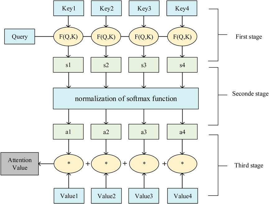
FIGURE 3. Steps of AM in MDACN.

A data-driven approach that incorporates an AM that assigns weights to different data allows the network to be trained faster. In addition, when employing the approach, since the network requires very little computational memory, it is also able to reason more efficiently during the training process.

3.3 Convolutional neural networks in proposed modal decomposition attentional convolutional network

The BiLSTM is employed to forecast the output of wind energy in complex terrain based on modal decomposition attention convolution network. Figure 4 shows the LSTM network structure. ${\mathrm{x}}_1\left(\mathrm{t}\right)$ and ${\mathrm{x}}_1\left(\mathrm{t}+1\right)$ are inputs. ${\mathrm{y}}_1\left(\mathrm{t}-1\right)$, ${\mathrm{y}}_1\left(\mathrm{t}\right)$ and ${\mathrm{y}}_1\left(\mathrm{t}+1\right)$ are outputs. $\mathrm{s}\left(\mathrm{t}-1\right)$ is previous memory element and, $\mathrm{s}\left(\mathrm{t}\right)$ is current memory element.

FIGURE 4

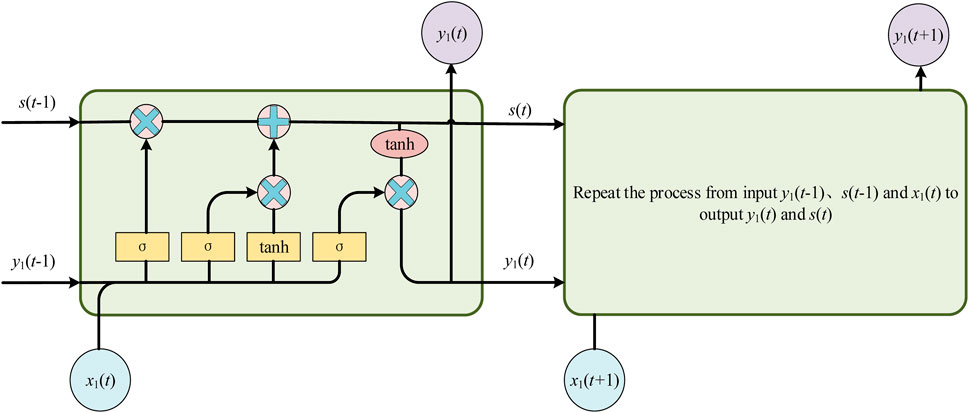
FIGURE 4. Structure of LSTM.

The BiLSTM network consists of two LSTM structures in opposite directions. The network has concealed layers in both positive and negative directions. Transmit two exports to two long and short memory networks in reverse orientations and concatenate their exports to form the ultimate export. Figure 5 presents the BiLSTM architecture.

FIGURE 5

FIGURE 5. Structure of BiLSTM in MDACN.

CNNs follow a forward transmission of information when learning. This type of processing does not do a good job of mining the valuable messages included in the wind turbine timesteps, and is not efficient. BiLSTM can effectively exploit existing historical and futuristic data to improve forecast accuracy. BiLSTM is a bi-directional loop based neural network with both positive and negative transmission mechanisms. BiLSTM then well compensates for the lack of information present in LSTM.

3.4 Application steps of the proposed modal decomposition attentional convolutional network for wind energy output forecast

Firstly, the original wind velocity and energy output data are modally decomposed by CEEMDAN, and the wind speed modal decomposition exports two modal constituents ${\mathrm{c}}_1\left(\mathrm{t}\right)$ and ${\mathrm{c}}_2\left(\mathrm{t}\right)$ with one remnant constituent ${\mathrm{x}}_3\left(\mathrm{t}\right)$. The modal components of wind speed decomposition are employed to predict the corresponding modal constituents of wind power output. After adding the attention weights, the information of these three wind velocity components is fed into the BiLSTM. To give an example with the modal component ${\mathrm{c}}_1\left(\mathrm{t}\right)$, convolution of the enter data of the current instant with the output data of the previous instant to obtain the attention goal. ${\mathrm{c}}_1\left(\mathrm{t}\right)$ is utilized to compute the value of the Query and ${\mathrm{y}}_1\left(\mathrm{t}-1\right)$ is utilized to compute the value of the Key. Next, the attentional goals are regularized and then multiplied with the input data in elemental order. Finally, the weighted data from AM is entered to BiLSTM for forecasting, and the ultimate results of the modal components are obtained. The predictions from the three parts are summed to produce the final wind energy output forecast. Figure 6 shows a partial structure of the BiLSTM network combined with the AM.

FIGURE 6

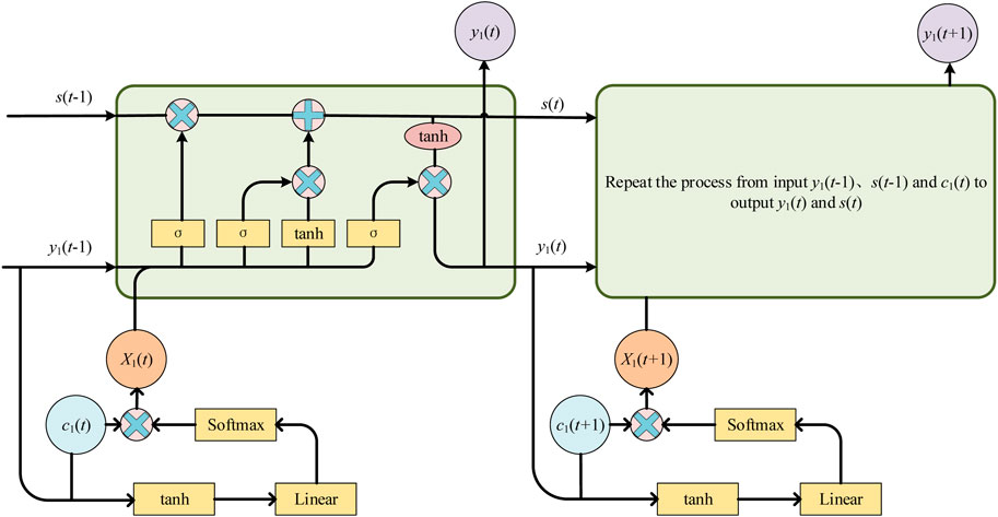
FIGURE 6. Partial structure of LSTM combined with AM in MDACN.

The advantages of the MDACN prediction approach are generalized as follows.

(1) The CEEMDAN algorithm gives higher accuracy by refining the original signal. Pattern decomposition is a noise elimination method that distills a mixture of features into several separate, independently predictable features.

(2) BiLSTM efficiently exploits characteristic messages in both directions by superposition with two LSTM levels. The method breaks through the restriction of forecasting the future time series based on the previous time series, and enables a greater convergence of export and situation.

(3) As the amount of data grows, the storage ability of RNN gradually reduces and fails to reflect long-time dependencies. AM is able to accurately determine the connection between the region and the whole prior to forecasting, thus simultaneously overcoming storage inefficiencies and increasing the forecasting accuracy.

4 Case studies

Experimental simulations are performed on MATLAB R2022a with a 2.10 GHz CPU and 32 GB on a 64-bit Windows 10 system. This experiment utilizes 9,072 sets of wind velocity and wind energy export data. Figure 7 shows the excerpted wind velocity and wind energy export data of 10 days. Because the intercepts are obtained from the wind velocity and wind energy export data at the same time, the wind energy export data have approximately the same pattern of ups and downs as the wind speed data indicating that the wind energy export is strongly influenced by the wind velocity. Therefore, the wind velocity data can be utilized to forecast the wind power output.

FIGURE 7

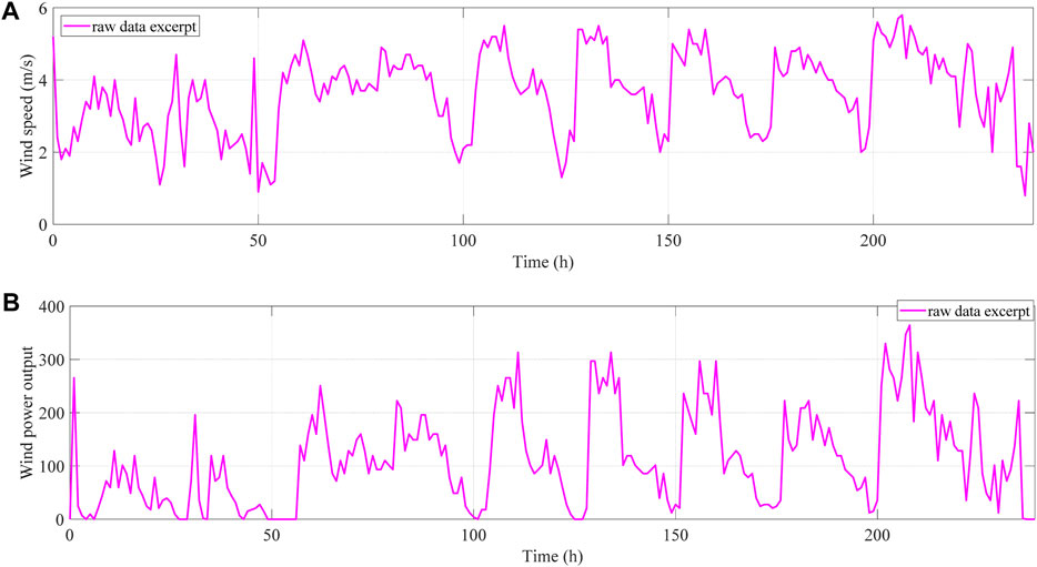
FIGURE 7. Data excerpts for 10 days: (A) wind velocity data; (B) wind energy export data.

First, the wind velocity and wind energy export data are decomposed by the same CEEMDAN, that is, the same white noise is added before each empirical modal decomposition for both types of data, and two modal components and one residual component are obtained respectively. If the amount of modal components is over set, the features may be corrupted, preventing the subsequent network from predicting accurately. If the amount of modal compositions is set too small, the features cannot be decomposed sufficiently to achieve the purpose of feature refinement. Figure 8 shows the three components of the wind speed data after decomposition. Figure 9 shows the three components of the wind energy export data after decomposition. The first two modal components are highly characterized parts of the raw signal, and extracting these parts, which are easy to find patterns, into a new signal for prediction can improve the prediction accuracy.

FIGURE 8

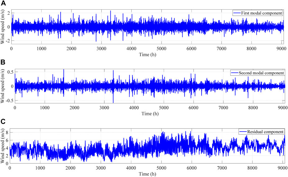
FIGURE 8. Three components of the wind speed data after decomposition: (A) first modal constituent; (B) second modal constituent; (C) residual constituent.

FIGURE 9

FIGURE 9. Three components of the wind power output data after decomposition: (A) first modal constituent; (B) second modal constituent; (C) residual constituent.

Figure 8 and Figure 9 show that the originally irregular data are decomposed into three sets of data with more regular ups and downs and more refined characteristics, thus allowing for more accurate predictions afterwards.

The MDACN prediction method is applied to each of the three modal components, and the modal decomposed wind speed modal component is employed to forecast the corresponding wind energy export modal component. 8,904 datasets are utilized as train sets and the remaining 168 datasets are utilized for testing sets. Table 1 shows the parameter settings of MDACN and the comparison methods. The solver utilizes stochastic gradient descent with momentum (SGDM). Compared to other solvers, SGDM converges better and the training process is more stable. According to the principle of control variables, the same parameters are utilized for all four methods. If max epochs is set too large, the model is likely to be overfitted and more time and computational resources are consumed, although the results may not be significantly improved. If max epochs is set too low, the network can fail to capture patterns and features in the training data, resulting in insufficient training and poor model performance. If the mini batch size is set too small, more time is spent, the gradient oscillation is severe, and the network is not favorable for convergence. Too large a mini batch size causes the network to easily fall into local minima. If the initial learn rate is too large, the loss function may diverge. If the initial learn rate is too small, the training speed will be very slow. Excessive hidden layer neurons will increase the computational power of the network and cause overfitting problem. If the number of neurons is too small, the desired effect will not be achieved.

TABLE 1

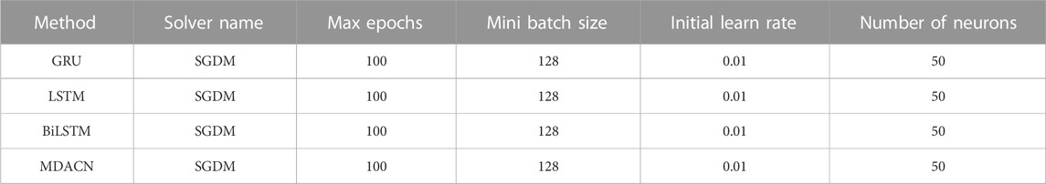
TABLE 1. Parameterization of MDACN and comparison methods.

Figure 10 presents the prediction outcomes for the three modal components. Comparison of raw and predicted data shows that the signal prediction after decomposition is effective, and the prediction curve and the raw data curve are basically coincident. Modal decomposition has a positive impact on signal prediction.

FIGURE 10

FIGURE 10. Forecasting results for the three modal constituents: (A) first modal constituent; (B) second modal constituent; (C) residual constituent.

Finally, the forecast outcomes of the three modal compositions are summed up and the ultimate results are composed with those predicted by the LSTM, GRU and BiLSTM models individually (Figure 11). Figure 11 indicates that the forecast value curve of the MDACN prediction method has a higher degree of overlap with the real value curve, suggesting that the MDACN has a high forecast accuracy.

FIGURE 11

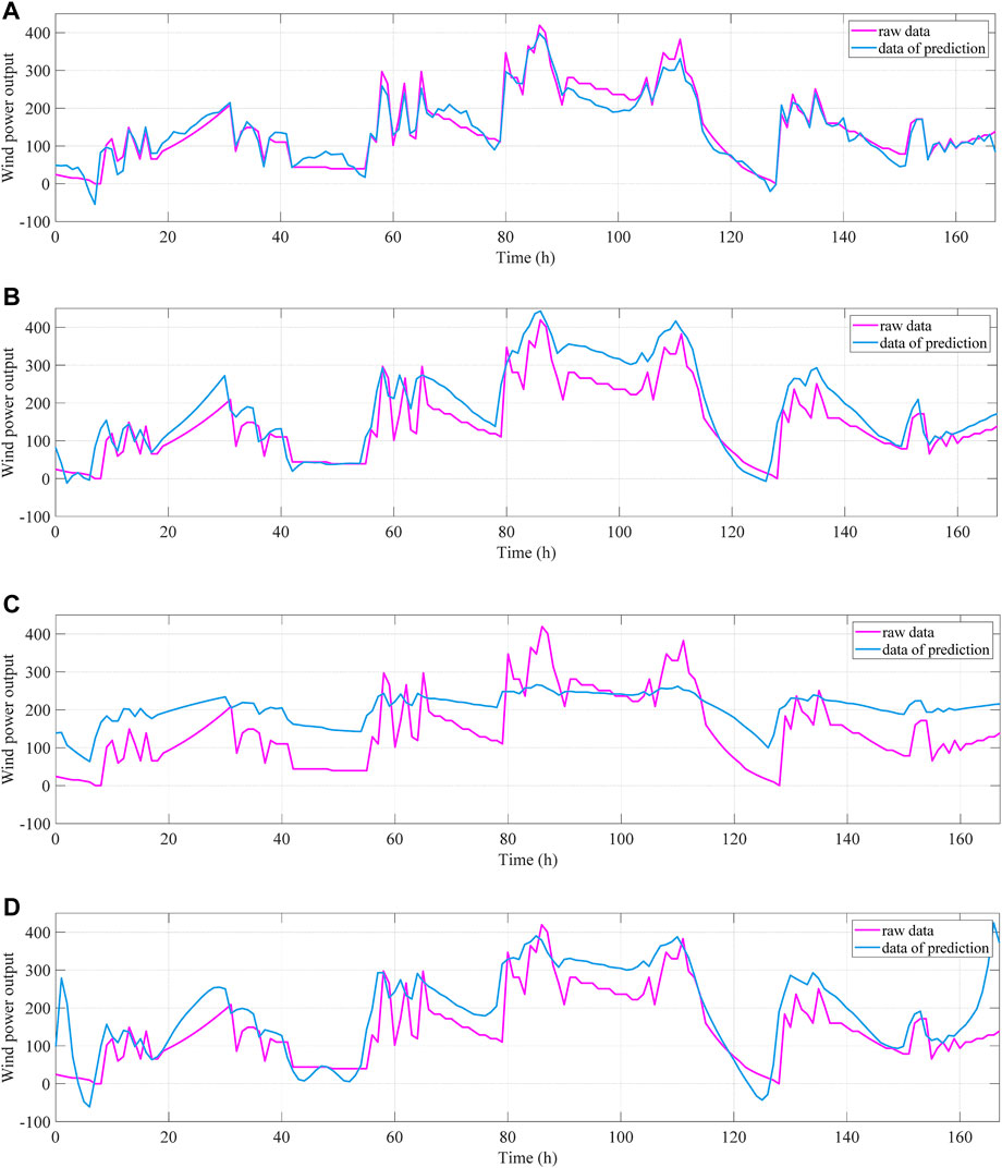
FIGURE 11. Forecasting results compared to the raw data: (A) MDACN; (B) GRU; (C) LSTM; (D) BiLSTM.

The results of the four prediction methods are calculated separately for the six prediction indicators proposed in this work (Table 2) and the fault profiles of the four forecasting approaches (Figure 12).

TABLE 2

TABLE 2. Fault indexes of the four forecasting approaches.

FIGURE 12

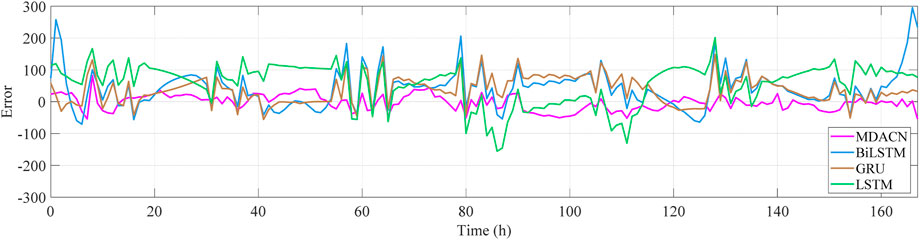
FIGURE 12. Fault profiles of the four forecasting approaches.

As can be seen in Table 1 and Figure 12, the MDACN method minimizes all error indicators and has a slicker error curve that is approaching the zero level. This indicates that the forecasting outcome of the MDACN produces small error and high accuracy, and it also indicates that the model of the MDACN is well fitted.

In order to verify the importance of AM and CEEMDAN in the MDACN approach, some ablation experiments are performed in this work. The AM in the MDACN method is first removed, and the raw signal after modal decomposition is predicted with BiLSTM. The forecasting outcomes of modal constituents predicted by BiLSTM (Figure 13) are compared with the forecasting outcomes of modal constituents predicted by MDACN (Figure 10), and the forecasting outcomes of the BiLSTM are less accurate in the part of the signal that has a large undulation. For the prediction of modal components, BiLSTM is not as accurate as the MDACN method.

FIGURE 13

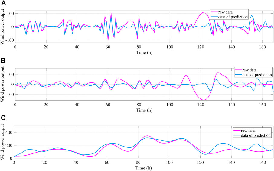
FIGURE 13. Prediction results of the three modal components with BiLSTM: (A) first modal constituent; (B) second modal constituent; (C) residual constituent.

The CEEMDAN in the MDACN method is removed, and the raw signals are directly predicted by the BiLSTM network with the AM added. Figure 14 shows the outcome of the ablation experiments contrasted to the MDACN forecasts. The overlap between the predicted and true curves is not as high as in the MDACN method, whether AM or CEEMDAN is subtracted, indicating that both AM and CEEMDAN perform an important role in the MDACN method.

FIGURE 14

FIGURE 14. Comparison of the forecasting outcomes of the ablation experiment and MDACN method: (A) MDACN; (B) MDACN without CEEMDAN; (C) MDACN without AM.

Table 3 shows the comparison of the evaluation indexes between the ablation experiments and the MDACN method. All six evaluation metrics of the MDACN method have smaller errors than the evaluation metrics of the ablation experiments, indicating the superior performance of the MDACN model. AM and CEEMDAN contributed a beneficial role to the high accuracy of the results.

TABLE 3

TABLE 3. Evaluation indexes of the ablation experiments and the MDACN method.

5 Conclusion

Wind power output is influenced by complex terrain and climate imposing many burdens on the dispatch of power systems. This work proposes a method that combines modal decomposition, AM and CNN for fast and accurate prediction of wind energy export in complex terrain. The MDACN prediction method is emulated and evaluated in comparison with the other three models, and the outcomes show the MDACN proposed in this paper achieves more accurate outcomes in forecasting the export of wind energy from complex terrains. This work describes the following.

(1) This work in used a modal decomposition approach. modal decomposition removes noise from the raw data and refines the mixture of features into distinct features that can be predicted individually. The data-driven approach combined with modal decomposition enables more accurate prediction of wind energy output.

(2) This work combines the AM algorithm with BiLSTM networks. AM relieves the network processing pressure, speeds up network training, and reduces the dependency of the network on computational memory. The BiLSTM network surmounts the restriction of a single data-driven model by adopting a deep fully-connected layer to surmount the disadvantage of low accuracy of a single data-driven model.

(3) The MDACN prediction approach has higher accuracy and improved system fitting in comparison to the forecasting of other CNN models individually.

In the next study, i) find the modal decomposition method that works better and enables more accurate and distinctive data after modal decomposition. ii) Keep improving the model structure and the methodology employed to continue to increase the reliability of the forecasting accuracy. iii) Simplify the structure of the model. For example, the operation of predicting and then adding the three modal components separately is complicated, and the structure needs to be simplified for improving the speed of model prediction.

Data availability statement

The data analyzed in this study is subject to the following licenses/restrictions: Extranet site. Requests to access these datasets should be directed to https://download.csdn.net/download/lt731512320/15469796.

Author contributions

All authors listed have made a substantial, direct, and intellectual contribution to the work and approved it for publication.

Acknowledgments

Item Number: 036000KK52220039 (GDKJXM20220889).

Conflict of interest

Authors YL, PX, YY, QL, and GW were employed by Guangdong Power Grid Limited Liability Company Power Dispatch Control Center.

Authors XM, CZ, and XH were employed by Southern Power Grid Digital Grid Group Co., Ltd.

Publisher’s note

All claims expressed in this article are solely those of the authors and do not necessarily represent those of their affiliated organizations, or those of the publisher, the editors and the reviewers. Any product that may be evaluated in this article, or claim that may be made by its manufacturer, is not guaranteed or endorsed by the publisher.

References

Ashtiani, F., Alexander, J. G., and Aflatouni, F. (2022). An on-chip photonic deep neural network for image classification. Nature 606, 501–506. doi:10.1038/s41586-022-04714-0

PubMed Abstract | CrossRef Full Text | Google Scholar

Balderas, D., Ponce, P., and Molina, A. (2019). Convolutional long short term memory deep neural networks for image sequence prediction. Expert Syst. Appl. 122, 152–162. doi:10.1016/j.eswa.2018.12.055

CrossRef Full Text | Google Scholar

Chen, H., Birkelund, Y., and Zhang, Q. (2021). Data-augmented sequential deep learning for wind power forecasting. Energy Convers. Manag. 248, 114790. doi:10.1016/j.enconman.2021.114790

CrossRef Full Text | Google Scholar

Deng, W., Li, Y., Huang, K., Wu, D., Yang, C., and Gui, W. (2023). LSTMED: an uneven dynamic process monitoring method based on LSTM and Autoencoder neural network. Neural Netw. 158, 30–41. doi:10.1016/j.neunet.2022.11.001

PubMed Abstract | CrossRef Full Text | Google Scholar

GuZhaoJian, X. H. L. (2022). Sequence neural network for recommendation with multi-feature fusion. Expert Syst. Appl. 210, 118459. doi:10.1016/j.eswa.2022.118459

CrossRef Full Text | Google Scholar

Harbola, S., and Coors, V. (2019). One dimensional convolutional neural network architectures for wind prediction. Energy Convers. Manag. 195, 70–75. doi:10.1016/j.enconman.2019.05.007

CrossRef Full Text | Google Scholar

He, F., Zhou, J., Mo, Li, Feng, K., Liu, G., and He, Z. (2020). Day-ahead short-term load probability density forecasting method with a decomposition-based quantile regression forest. Appl. Energy 262, 114396. doi:10.1016/j.apenergy.2019.114396

CrossRef Full Text | Google Scholar

Kulshrestha, A., Krishnaswamy, V., and Sharma, M. (2020). Bayesian BILSTM approach for tourism demand forecasting. Ann. Tour. Res. 83, 102925. doi:10.1016/j.annals.2020.102925

CrossRef Full Text | Google Scholar

Lin, C.-P., Cabrera, J., Yang, F., Ling, M.-Ho, Tsui, K.-L., and Bae, S.-J. (2020). Battery state of health modeling and remaining useful life prediction through time series model. Appl. Energy 275, 115338. doi:10.1016/j.apenergy.2020.115338

CrossRef Full Text | Google Scholar

Liu, H., Yang, L., Zhang, B., and Zhang, Z. (2023). A two-channel deep network based model for improving ultra-short-term prediction of wind power via utilizing multi-source data. Energy 283, 128510. doi:10.1016/j.energy.2023.128510

CrossRef Full Text | Google Scholar

Liu, H., and Zhang, Z. (2022). A bilateral branch learning paradigm for short term wind power prediction with data of multiple sampling resolutions. J. Clean. Prod. 380, 134977. doi:10.1016/j.jclepro.2022.134977

CrossRef Full Text | Google Scholar

Liu, X., Yang, L., and Zhang, Z. (2021). Short-term multi-step ahead wind power predictions based on a novel deep convolutional recurrent network method. IEEE Trans. Sustain. Energy 12 (3), 1820–1833. doi:10.1109/tste.2021.3067436

CrossRef Full Text | Google Scholar

Liu, X., Yang, L., and Zhang, Z. (2022). The attention-assisted ordinary differential equation networks for short-term probabilistic wind power predictions. Appl. Energy 324, 119794. doi:10.1016/j.apenergy.2022.119794

CrossRef Full Text | Google Scholar

López-Oriona, Á., and Vilar, J. A. (2021). Outlier detection for multivariate time series: a functional data approach. Knowledge-Based Syst. 233, 107527. doi:10.1016/j.knosys.2021.107527

CrossRef Full Text | Google Scholar

Lv, Y.-jun, Wang, J.-wei, Wang, J., Cheng, X., Zou, L., Li, Ly, et al. (2020). Steel corrosion prediction based on support vector machines. Chaos, Solit. Fractals 136, 109807. doi:10.1016/j.chaos.2020.109807

CrossRef Full Text | Google Scholar

Ma, Y., Li, Y. P., and Huang, G. H. (2023). Planning China’s non-deterministic energy system (2021–2060) to achieve carbon neutrality. Appl. Energy 334, 120673. doi:10.1016/j.apenergy.2023.120673

CrossRef Full Text | Google Scholar

Qi, Ye, Liu, T., and Jing, L. (2023). China's energy transition towards carbon neutrality with minimum cost. J. Clean. Prod. 388, 135904. doi:10.1016/j.jclepro.2023.135904

CrossRef Full Text | Google Scholar

Qian, G.-W., and Ishihara, T. (2022). A novel probabilistic power curve model to predict the power production and its uncertainty for a wind farm over complex terrain. Energy 261, 125171. doi:10.1016/j.energy.2022.125171

CrossRef Full Text | Google Scholar

Shahid, F., Zameer, A., and Muneeb, M. (2020). Predictions for COVID-19 with deep learning models of LSTM, GRU and Bi-LSTM. Chaos, Solit. Fractals 140, 110212. doi:10.1016/j.chaos.2020.110212

PubMed Abstract | CrossRef Full Text | Google Scholar

Shang, Z., Chen, Y., Chen, Y., Guo, Z., and Yang, Yi (2023). Decomposition-based wind speed forecasting model using causal convolutional network and attention mechanism. Expert Syst. Appl. 223, 119878. doi:10.1016/j.eswa.2023.119878

CrossRef Full Text | Google Scholar

Shi, H., Qin, C., Xiao, D., Zhao, L., and Liu, C. (2020). Automated heartbeat classification based on deep neural network with multiple input layers. Knowledge-Based Syst. 188, 105036. doi:10.1016/j.knosys.2019.105036

CrossRef Full Text | Google Scholar

Sun, C., He, Z., Lin, H., Cai, L., Cai, H., and Gao, M. (2023). Anomaly detection of power battery pack using gated recurrent units based variational autoencoder. Appl. Soft Comput. 132, 109903. doi:10.1016/j.asoc.2022.109903

CrossRef Full Text | Google Scholar

Tang, G., Li, Bo, Dai, H.-N., and Zheng, Xi (2022). SPRNN: a spatial–temporal recurrent neural network for crowd flow prediction. Inf. Sci. 614, 19–34. doi:10.1016/j.ins.2022.09.053

CrossRef Full Text | Google Scholar

Wang, Q., Luo, K., Wu, C., Zhu, Z., and Fan, J. (2022). Mesoscale simulations of a real onshore wind power base in complex terrain: wind farm wake behavior and power production. Energy 241, 122873. doi:10.1016/j.energy.2021.122873

CrossRef Full Text | Google Scholar

Wang, Y., Deng, L., Zheng, L., and Robert, X. (2021). Temporal convolutional network with soft thresholding and attention mechanism for machinery prognostics. J. Manuf. Syst. 60, 512–526. doi:10.1016/j.jmsy.2021.07.008

CrossRef Full Text | Google Scholar

Yang, T., Xia, Yu, Ning, Ma, Zhang, Y., and Li, H. (2022). Deep representation-based transfer learning for deep neural networks. Knowledge-Based Syst. 253, 109526. doi:10.1016/j.knosys.2022.109526

CrossRef Full Text | Google Scholar

Yildiz, C., Acikgoz, H., Korkmaz, D., and Budak, U. (2021). An improved residual-based convolutional neural network for very short-term wind power forecasting. Energy Convers. Manag. 228, 113731. doi:10.1016/j.enconman.2020.113731

CrossRef Full Text | Google Scholar

Yin, L., and Xie, J. (2021). Multi-temporal-spatial-scale temporal convolution network for short-term load forecasting of power systems. Appl. Energy 283, 116328. doi:10.1016/j.apenergy.2020.116328

CrossRef Full Text | Google Scholar

Yin, S., and Liu, H. (2020). Wind power prediction based on outlier correction, ensemble reinforcement learning, and residual correction. Energy 250, 123857. doi:10.1016/j.energy.2022.123857

CrossRef Full Text | Google Scholar

Zheng, Z., and Zhang, Z. (2023). A stochastic recurrent encoder decoder network for multistep probabilistic wind power predictions. IEEE Trans. Neural Netw. Learn. Syst., 1–14. Early Access. doi:10.1109/tnnls.2023.3234130

CrossRef Full Text | Google Scholar

Zhou, F., Huang, Z., and Zhang, C. (2022). Carbon price forecasting based on CEEMDAN and LSTM. Appl. Energy 311, 118601. doi:10.1016/j.apenergy.2022.118601

CrossRef Full Text | Google Scholar