A carbon metering method for distribution networks considering harmonic influences

Harmonics brought about by a large number of impulsive and non-linear loads connected to the grid has led to new challenges in regional carbon emission management. The existence of harmonics increases the consumption of power equipment, and the transformation of signal forms makes the accuracy of carbon measurement questioning, which damages fairness and is not conducive to a carbon trading market construction and the purpose of precise carbon verification. This paper proposes that the harmonic level of each node is monitored during carbon metering of the distribution network; carbon metering results are corrected based on the correction amount of harmonic carbon. Harmonic separation and electric carbon conversion of the current-containing harmonic source are conducted on the IEEE-33 node. The results show that harmonic carbon does exist. Carbon metering results are affected when the power quality is seriously distorted, which is not conducive to establishing a carbon metering trading market.

1 Introduction

Global warming is one of the challenges human society is facing today. The role of CO₂ in the global warming effect caused by greenhouse gases is as high as 77% (Kweku et al., 2018). Therefore, reducing CO₂ emissions is an urgent issue. Over the past decades, various countries have been making efforts to reduce carbon emissions, and China has released an action plan to reach the peak of CO₂ emissions by 2030 (Fang et al. 2019). Specifically, the power industry accounts for a huge share of carbon emissions, and therefore, accurate carbon emission metering is crucial.

Generally, the existing carbon emission calculation methods (Zhang et al. 2021a) are based on the statistics of energy consumption. Specifically, carbon emission data are obtained by multiplying power generation and carbon emission factors. It has the advantages of simple calculation and practical methods. However, this approach cannot reflect the low carbon characteristics of the power system. The power system carbon emission flow (PSCEF) (Kang et al., 2012; Sun K et al., 2023; Kang et al., 2015; Sun et al., 2017) is defined as a virtual network flow that is dependent on the power flow (PF), and it is used to characterize the carbon emissions that maintain the power flow in either branch. Specifically, the PSCEF is equivalent to labeling the current on each branch with carbon emissions. In the power system, the carbon emission flow starts from the power plant, enters the power system from the power plant’s feeder, follows the power in the system, and finally, flows to the customerterminal on the customer side.

The PSCEF effectively maps the relationship between electricity and carbon conversion. Based on this, scholars have conducted research and improvements. Wang et al. (2022) proposed a demand response (DR)-based low-carbon optimal-scheduling model for carbon intensity control. Meanwhile, a data-driven approach based on deep learning (Qin et al. 2022) is utilized for carbon emission flow (CEF) modeling to cope with the shortcomings of conventional emission calculations. Cheng et al. (2018) proposed a carbon emission stream analysis model for multi-energy management systems to quantify the carbon emissions associated with energy transport and conversion processes. An optimal scheduling model of an integrated energy system is proposed to verify the impact of carbon emissions on system scheduling and LMP (Jiang et al., 2018). However, the aforementioned theories and their improvement methods are only on how to make mapping more realistic. In real applications, the construction of carbon markets (Zhou and Li, 2019) involving user transactions cannot be separated from accurate carbon measurement methods. Although the accuracy of carbon flow calculations has been improving all the time, this does not guarantee the accuracy of carbon measurement results. With a low-carbon goal, a large amount of new energy generation and power electronics are connected to the grid, making the power quality unreliable. Correlated regional loads and unpredictable renewable energies in the power system make regional carbon emission management (RCEM) increasingly challenging and necessary (Wang et al., 2015). The degraded power data will inevitably lead to errors in carbon measurement results (Suo et al., 2022). Furthermore, carbon measurement results affected by harmonics will be questioned by many parties when it comes to low-carbon responsibility delineation and metering transactions.

Currently, harmonic PF calculations in distribution networks (Sun H et al., 2023) are emerging. Lundquist and Bollen (2000) were the first to show the principle that harmonic active power in radial low- and medium-voltage distribution systems varies due to the interaction between the load and the power system. Zhang and Wang (2014) proposed a forward/backward sweeping distribution system harmonic power flow algorithm based on the output impedance model considering the interaction between the DG and the grid. Some scholars also proposed a harmonic power flow calculation method for distribution networks based on a general model of harmonic sources based on the network topology (Zhang et al., 2021b). In summary, the harmonic source is regarded as a single-port unknown network, and the voltage–current relationship in the time domain is converted into an expression in the frequency domain. Using the superposition theorem and triangular relations, matrix relations of the general model of the harmonic source are established. The harmonic derivative equation and the harmonic source model equation of the system are also solved to obtain the harmonic power flow of the system.

In order to investigate the effect of harmonics on carbon metering in distribution networks, this paper proposes a correction method for carbon flow calculations combined with harmonic PF calculations. Specifically, first, the carbon emission factor at the beginning of distribution network nodes is obtained by the main network carbon flow calculation. Then, the harmonic currents of the distribution network are calculated using the decoupling method (Ulinuha et al. 2007; Canesin et al. 2014) to obtain the harmonic distortion rate of each node. Finally, the correction measurement of harmonic carbon is carried out for nodes whose distortion crosses the limit.

2 Harmonic power flow

In the case where the distribution network contains non-linear loads or non-linear substation equipment, the power flow in the system consists of the fundamental power flow and harmonic power flow. Unlike the fundamental power flow, the harmonic power flow is derived from non-linear loads and substation equipment.

In order to analyze the effect of harmonics on the carbon flow in power systems, it is necessary to analyze the carbon flow corresponding to harmonics. To analyze the harmonic carbon flow, first, the harmonic source should be reasonably simplified and modeled and the parameters of the harmonic source should be determined through an analysis; after that, the distribution of the harmonic power flow in the system is required, and the harmonic carbon flow analysis is carried out on the basis of the distribution of the harmonic power flow.

In the actual system, the presence of harmonics derives metering results from the ideal power flow default for carbon flow calculations, resulting in inaccurate node carbon measurements. The formula for the power signal without the DC component is shown in Eq. 1. Assuming that the fundamental wave is the first harmonic, the power signal consists of the fundamental and each high-frequency harmonic and Gaussian white noise.

$f\left(t\right)=\sum _{h=1}^{\infty }{A}_{h}cos\left(2\pi f_{h}t+{\phi }_h\right)+noise,(1)$

where A_h, f_h, and φ_h are the magnitude, frequency, and phase of the harmonic signal, respectively.

2.1 Harmonic source model

To characterize the harmonic current generated by a harmonic source, the harmonic source needs to be modeled. The harmonic currents generated can be expressed as a function of the node voltage and load control parameters.484 (IEEE, 1996)

$I_k=F_k\left(U_1,U_2,\dots U_n,C_1,C_2,\dots C_n\right),(2)$

where k = 1, 3, 5, …, n, and n is the number of harmonics; I_k is the kth-harmonic current generated by the non-linear load; U₁, U₂, …, U_n are the fundamental and harmonic component of the node voltage of the non-linear load; C₁, C₂, …, C_n are the load control parameters. They are the circuit structure and control parameters of the device for the first category of harmonic sources and the parameters characterizing the voltammetric characteristics for the second category of harmonic sources. Theoretically, Eq. 2 is an accurate model of harmonic sources, but the model is too complicated for calculation, which limits its application in harmonic analysis and calculation.

In this study, the Norton model is used to characterize the current characteristics of the harmonic source. The basic idea of the Norton harmonic source model is to consider the non-linear load as a harmonic current source, which can be described as a current source in series with an equivalent impedance. In this model, the harmonic current source is considered to exist independently in the power system and is not influenced by voltage variations. The equivalent impedance of the harmonic current source is determined by the non-linear load and system impedance in parallel with it.

$I_k=I_{k0}+\frac{U_k}{Z_k}.(3)$

I_k0 is determined by the fundamental voltage at the node where the harmonic source is located. U_k and Z_k are the kth-harmonic voltage and kth-harmonic impedance, respectively. Z_k and I_k0 are calculated by Eqs. 4, 5, respectively, and i and j represent the measurement results of different operating conditions of the system.

$Z_K=\left|\frac{V_{k,i}-V_{k,j}}{I_{k,i}-I_{k,j}}\right|,(4)$

$I_{k0}=I_{k,i}+\frac{V_{K,i}}{Z_k}.(5)$

2.2 Harmonic power flow calculation

Due to the coupling relationship between the fundamental power flow and harmonic power flow, the influence of the fundamental power flow on the harmonic power flow is large. However, the influence of the harmonic power flow on the fundamental power flow is small. Therefore, the analysis of the fundamental power flow is the main aspect. The fundamental power flow is calculated first, and the harmonic current is solved later. The effect of the harmonic power flow is not considered in the calculation of the fundamental power flow, and its effect on the harmonic power flow is known after the calculation of the fundamental power flow. In this way, the decoupling of the fundamental and harmonic power flow is achieved.

Because the decoupling algorithm ignores the effect of each harmonic voltage on the fundamental current of the harmonic source, fundamental and harmonic currents of the harmonic source can be expressed, respectively, as follows:

$I_1=F_1\left(U_1\right),(6)$

$I_n=F_n\left(U_1,U_2,\dots \right);n=\mathrm{2,3}\dots .(7)$

When the decoupling algorithm calculates the fundamental power flow, for the linear load bus, its fundamental injection power is dependent on the bus where it is located. For the harmonic source bus, the amplitude and phase of its fundamental current can be derived using Eq. 6, and then, its fundamental active and reactive power can be calculated. Since the fundamental voltage is continuously updated during the iteration of the fundamental current, the fundamental current should be recalculated using Eq. 6 for all iterations of the fundamental current to update the fundamental active and reactive power absorbed by the harmonic source.

After the calculation of the fundamental power flow is completed, the fundamental voltage U1 is known. In Eq. 7, if each harmonic voltage is zero, then the initial value of each harmonic current injected into the grid by the harmonic power flow can be found. According to the bus voltage equation,

$I_n=Y_n{U}_n.(8)$

From the aforementioned equation, the harmonic voltage of each bus of the system can be obtained, and then, the harmonic voltage is substituted into Eq. 7 to obtain the correction value of each harmonic current of the harmonic source. The new harmonic voltages are obtained by substituting the corrected values of harmonic currents into Eq. 8. This iteration is repeated until a given convergence accuracy is satisfied.

3 Carbon flow theory and the harmonic carbon flow

The carbon flow theory is proposed to quantify the state of carbon emissions in a power system based on the distribution of the power flow. The power system carbon flow is a kind of virtual network flow that depends on the power flow and is used to characterize the carbon emission distribution in the power system. The power system carbon flow is equivalent to labeling each PF with carbon emissions. The carbon flow in the power system originates in the power plant and eventually enters load nodes via the power grid. Similar to electricity, the carbon flow is generated by generators. It is consumed by electricity consumers through the carbon flow. Correspondingly, the harmonic carbon flow is a measure of carbon emissions based on harmonics in the power system to correct the emissions of each load in each branch of the system.

3.1 Concepts to describe carbon emissions

The calculation of the carbon flow is used to measure the production, consumption, and transmission of carbon in the power system. Some basic concepts of the carbon flow are introduced as follows, including the carbon flow, carbon flow rate, and carbon flow density (CFD). The CFD is defined to describe the relationship between the carbon flow and active power in power systems. Furthermore, the CFD is divided into two categories according to the branch and node, namely, the branch carbon flow density and the node carbon potential, respectively.

3.1.1 Carbon flow and the carbon flow rate

The carbon flow is a basic concept in the carbon flow theory. The carbon flow characterizes the magnitude of the carbon flow in a branch or load, which is represented by F. The carbon flow is defined as the cumulative amount of carbon emissions in a given branch or load. The international unit of carbon emissions is generally expressed in tCO₂ or kgCO₂.

The carbon flow rate is defined as the carbon flow that passes the branch or flows into the load per unit time, represented by R, at a value equal to the derivative of the carbon flow rate with respect to time as shown in the following equation:

$R=\frac{\mathrm{d}F}{\mathrm{d}t}.(9)$

3.1.2 Branch carbon flow density

Given that the carbon emission flow of the power system is dependent on the PF, it is necessary to combine the carbon emission flow with the PF. Furthermore, the carbon emission in the power system is mainly related to active power. To characterize the combination of them both, the ratio of the carbon flow rate of any branch to active power is defined as the branch carbon flow density (BCFD).

$\rho =\frac{R}{P},(10)$

where ρ represents the ratio of the CFR of any branch to the active PF in the power system.

The unit of the carbon flow density is gCO₂/(kWh). In generator nodes, the BCFD is equal to the carbon emission intensity of the generator. In the load, the BCFD is equal to the carbon emission value of the generation side caused by the consumption of unit power transmitted by the branch line.

3.1.3 Node carbon potential

The carbon flow theory defines the physical quantity that describes the carbon emission intensity of nodes by the carbon emission flow, named the node carbon potential (NCP). e_n is used to describe the NCP of node n.

$e_n=\frac{{\sum }_{i\in N^{+}}{P}_i{\rho }_i}{{\sum }_{i\in N^{+}}{P}_i}=\frac{{\sum }_{i\in N^{+}}{R}_i}{{\sum }_{i\in N^{+}}{P}_i},(11)$

where the unit of the NCP is gCO₂/(kWh), the same as that of the BCFD. The NCP equals the weighted average of BCFD ρ_it of all branches flowing into node n concerning active power P_it.

The physical meaning of the NCP is the value of carbon emissions caused by the consumption of a unit of electricity on that bus. For a power plant bus, its nodal carbon potential is equal to the real-time generation carbon emission intensity of a power plant.

3.2 Node carbon potential vector

The primary goal of carbon emission flow calculations in a power system is to calculate the carbon potential of all nodes. To calculate the fundamental node carbon potential vector (FNCPV), three matrices should be constructed first. Specifically, these matrices are the fundamental node active flux matrix (P_NF), fundamental branch power flow distribution matrix (P_BF), and generator injection distribution matrix (P_G). Furthermore, they are constructed from power flow calculation results. To calculate the harmonic carbon potential vector (HNCPV), three matrices should be constructed as well; they are the harmonic node active flux matrix (P_NH), harmonic branch power flow distribution matrix (P_BH), and harmonic source injection distribution matrix (P_HS). The FNCP and HNCP of the power system can be calculated based on the aforementioned results.

•P_NF and P_NH are N-order diagonal matrices that describe the contribution of the generator set and other nodes to the NCP of a node in the system; the subscripts here and later F and H denote the terms fundamental and harmonic, respectively.

•P_BF and P_BH are used to describe the active power flow distribution of the power system. This matrix contains the topology structure information of the power network and the steady-state active power flow distribution information.

•P_G is K times the N matrix. It is defined to describe the connection between all generating sets and the power system. In addition, it represents the active power injected into the system by the unit.

•E_G and E_HS are vectors representing the carbon potential of all generators and harmonic sources in a power system, respectively.

$E_{NF}={\left(P_{NF}-P_{BF}^T\right)}^{-1}{P}_G^T{E}_G,(12)$

$E_{NH}={\left(P_{NH}-P_{BH}^T\right)}^{-1}{P}_{HS}^T{E}_{HS}.(13)$

3.3 Total harmonic distortion of carbon

Once the amount of the harmonic carbon flow is calculated, it can be used to correct the fundamental carbon flow to obtain accurate carbon measurement results. R_BC is the corrected branch carbon flow rate, and it is calculated as follows:

$R_{BC}=R_{BF}+\sum _2^N{R}_{BH,N},(14)$

where N represents the number of harmonics.

In the previous carbon metering methods, only the fundamental carbon flow was considered and the problems caused by harmonics and their generated carbon flows were not considered. By calculating the harmonic carbon flow and summing it with the fundamental carbon flow, all the carbon flow that actually flows in each branch is calculated accurately. THD_CF is a parameter used to measure the effect of the harmonic carbon flow on the fundamental carbon flow, indicating the ratio of the harmonic carbon flow to the harmonic carbon flow. THD_CF and THD_I are calculated by Eqs. 15, 16, respectively, where N stands for the number of harmonics. THD_I is the total harmonic distortion of the current.

$TH{D}_{CF}=\frac{{\sum }_2^N{R}_{BH,N}}{R_{BF}},(15)$

$TH{D}_I=\sqrt{\sum _2^N{\left(\frac{I_N}{I_1}\right)}^2}.(16)$

4 Calculation framework of the harmonic carbon flow

This section proposes a calculation model to analyze the effect of harmonics on the carbon flow in a power system containing harmonics. The framework of this paper is shown in Figure 1, where the original nodal power signal is considered as a combination of fundamental and harmonic signals. First, the calculation computes the carbon potential of each node by carbon flow calculations. At the same time, harmonic distortion rate monitoring is executed to determine the harmonic level of the signal. If the threshold value is exceeded, the harmonic power flow is executed to calculate the harmonic energy. The harmonic energy is multiplied with the node carbon potential to obtain the harmonic carbon correction amount. Finally, the accurate carbon measurement value is obtained by summing fundamental carbon and harmonic carbon. E_G and E_HS are boundary conditions for the model; the carbon intensity of the generators, E_G, should be initialized; E_HS is the boundary condition for the harmonic carbon flow calculation determined after the fundamental harmonic carbon flow. Before the calculation, the carbon intensity of the generators should be initialized. Then, the following steps should be performed to calculate the harmonic carbon flow:

1. The first step is the decomposition of power system signals into fundamental and harmonics

2. The system fundamental power flow is calculated, and based on the active power distribution, we establish P_NF, P_BF, and P_G

3. If P_NF–P_BF is invertible, we go to step 5; otherwise, which means that the power system is not connected or there are siloed nodes, we go to step 4

4. Unconnected and siloed nodes are eliminated, and we go to step 1

5. We calculate E_NF for all nodes, R_BF for all branches, and E_NF of nodes where harmonic sources are located, which is the carbon emission intensity of harmonic sources

6. The harmonic power flow is calculated, and based on the active power distribution, we establish P_NH, P_BH, and P_HS

7. We calculate E_NH for all nodes and R_BH,N for all branches

8. We correct the branch carbon flow rate (R_BC) to get accurate carbon measurement results

FIGURE 1

FIGURE 1. Framework of precise carbon metering considering harmonics.

5 Results and discussion

To demonstrate the proposed method and model, a case study based on the IEEE-33 bus system is presented without considering the network loss and assuming that the system has no power exchange with the main grid. This system has two generators, one burns fossil fuels located on bus 1 and another is a new energy generator located on bus 18, which is also a harmonic source. A total of 32 buses carry a load, and there is only one voltage level for the whole system.

As shown in Figure 2, the harmonic source is located in node 5, node 13, node 23, and node 31. Harmonic sources generate the third, fifth, seventh, ninth, eleventh, and thirteenth harmonics. The magnitude of harmonics decreases as the number of harmonics increases. Given that G1 is a thermal power generator, its carbon potential is at a high level, while the new energy generator has a low carbon potential. We initialize the carbon potential of the thermal generator and new energy generator as 845 gCO₂/kWh and 0 gCO₂/kWh, respectively, which means $E_G=\left[\mathrm{875,0}\right]$. The carbon potential of harmonic sources depends on the carbon potential of the bus where they are located, so E_HS needs to be determined after the calculation of the fundamental carbon flow.

FIGURE 2

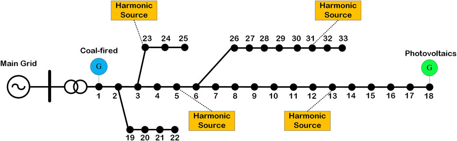
FIGURE 2. IEEE-33 standard system.

According to the calculation framework, the fundamental power flow and fundamental carbon flow are calculated first. The total harmonic distortion of voltage (THD_U) at each node is shown in Figure 3. The harmonic distortion of the 30th to 33rd nodes is the most serious, with a total distortion rate of more than 12%, and the distortion of all nodes is less than 15%.

FIGURE 3

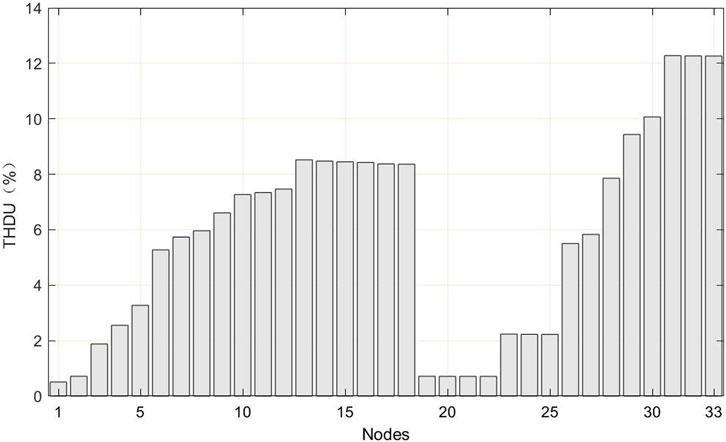
FIGURE 3. THD_U for all nodes.

Table 1 shows branch connections and fundamental carbon flow R_BF. The bus-to-bus flow is used to describe the branch connection and specify the direction of the branch, such as the carbon flow and power flow. If the carbon flow and power flow are the same as the direction, then the carbon flow or power flow values are positive; otherwise, they are negative. According to fundamental harmonic carbon flow calculation results, initial conditions for the calculation of the harmonic carbon flow, the harmonic source carbon potential (E_HS) is determined, $E_{HS}=\left[\mathrm{875,875,875,875}\right]$. This is because the power emitted by the generator is much greater than that of the distributed power source, so E_NF of the nodes far from the distributed power source is closer to E_G of the generator.

TABLE 1

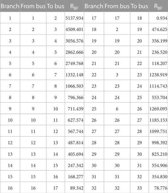
TABLE 1. Branch connection and the fundamental carbon flow (KgCO₂/s).

Along with the flow of each harmonic through branches of the system, the carbon flow in the branch will also consist of the corresponding carbon flow of each harmonic. Table 2 shows the harmonic carbon flow rate for all branches in the system. Since the power injected by harmonic sources decreases as the number of harmonics increases, the corresponding harmonic carbon flow also decreases as the number of harmonics increases. Since harmonic sources are located in a different location than the generators, the harmonic carbon flow does not flow in the same direction as the fundamental carbon flow in branches.

TABLE 2

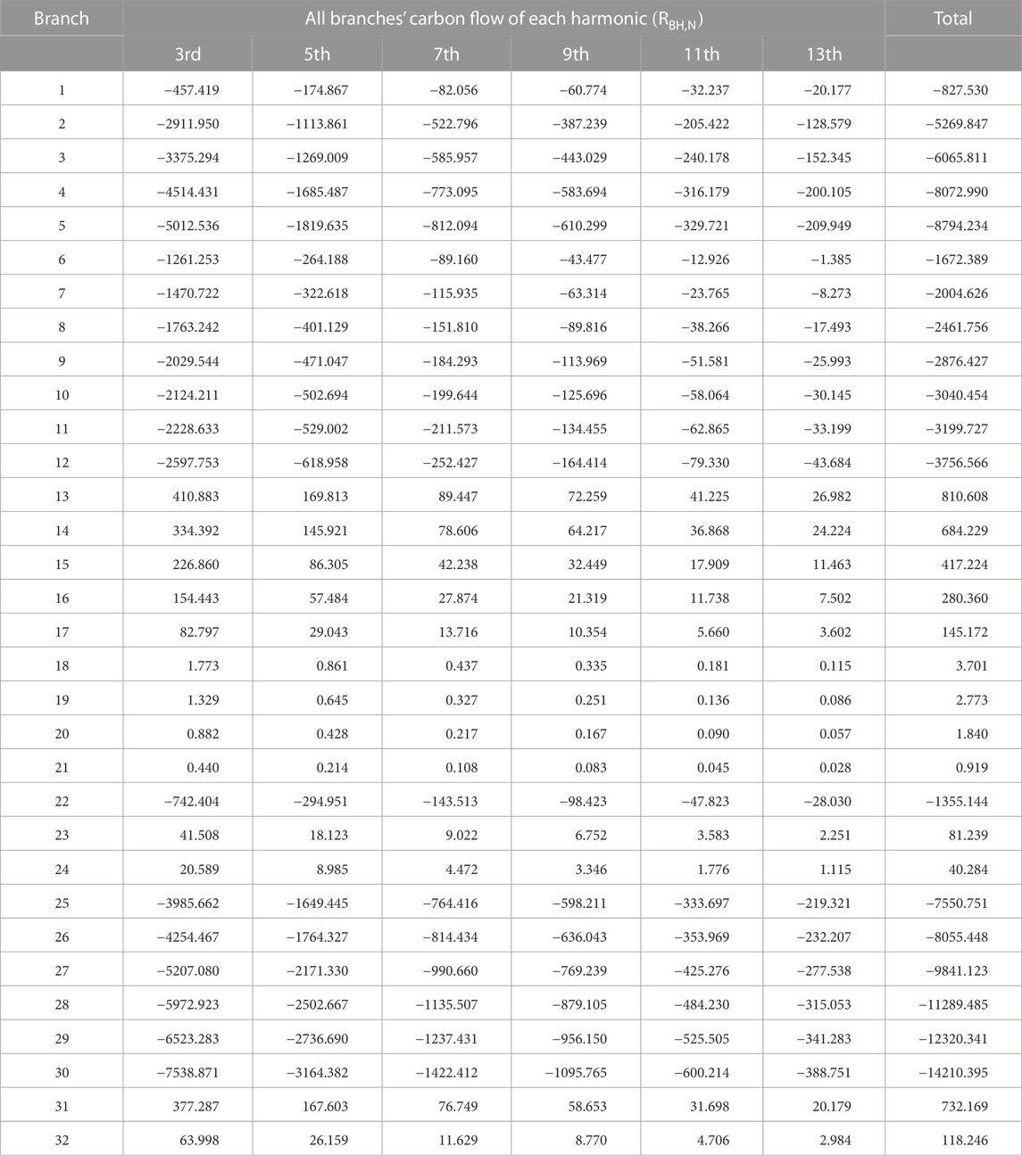
TABLE 2. R_BH of all branches (gCO₂/s).

As shown in Table 3, ${\sum }_2^N{R}_{BH,N}$ is the total carbon flow generated by the harmonic carbon flow. R_BC is the corrected carbon flow of all branches. In the 17th branch, ${\sum }_2^N{R}_{BH,N}$ and R_BC are in the same order of magnitude. Harmonics have a significant impact on the carbon flow in this branch.

TABLE 3

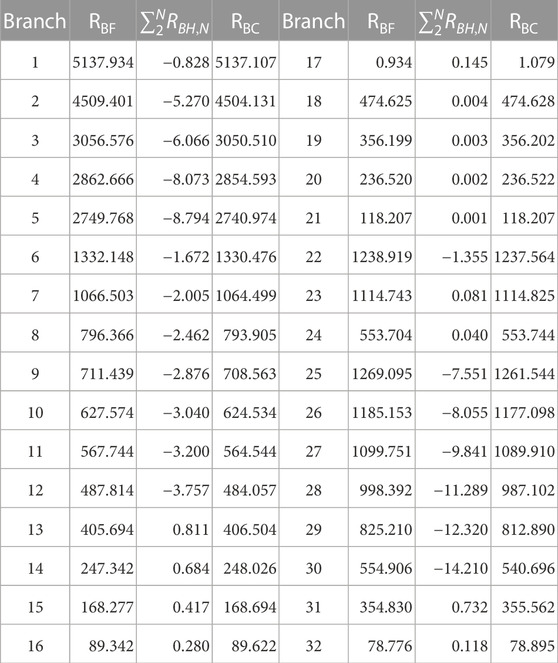
TABLE 3. Correction of the branch carbon flow rate (KgCO₂/s).

Figure 4 shows the total harmonic distortion of current (THD_I) and the total harmonic distortion of carbon flow (THD_CF). Although the calculation of the carbon flow is closely related to the active power of the branches, this system has only one voltage level; so this relationship can be seen as a relationship with the current. The distribution of the harmonic carbon flow distortion and harmonic current distortion in branches is not the same; the current distortion rate is very large, while the carbon flow distortion rate may still be very small. Therefore, the analysis of the branch harmonic carbon flow distortion cannot simply be considered as the branch current harmonic distortion, where the distortion of the current is not severe, but carbon flow distortions can be very serious, which can have a significant impact on the establishment of carbon markets and the fairness of carbon trading.

FIGURE 4

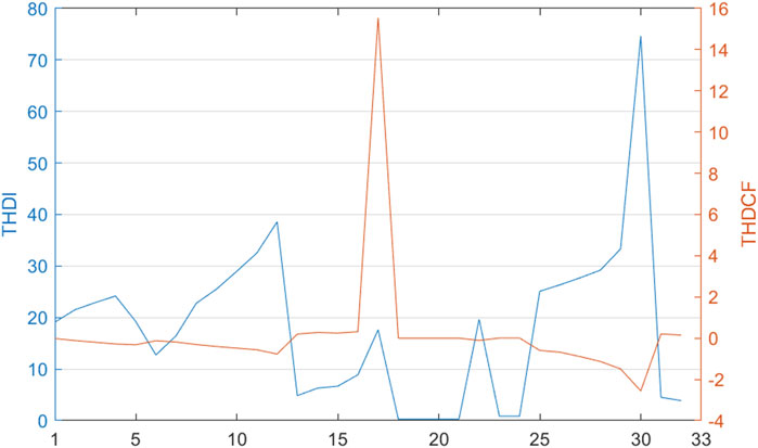
FIGURE 4. Total harmonic distortion of the current and the carbon flow for all branches.

6 Conclusion

This paper provides a novel analytical model for the carbon emission flow in the power system that contains harmonics. The model can improve the accuracy of power system carbon emission measurement and clarify the effect of harmonics on the carbon flow. The carbon flow exists as a virtual network flow dependent on the power flow, generated in the generator and transmitted in the transmission network. Due to the large number of new energy sources connected to the grid and the increase of non-linear power electronic equipment loads, the harmonic problem of the power system has become more and more evident. The issue of the accuracy of carbon measurement and the fairness of carbon trading has also arisen. The harmonic carbon flow calculation model calculates the distribution of the harmonic carbon flow for power systems containing harmonics and is able to make corrections to the carbon flow of the power system. The model is verified by the IEEE-33 bus system.

Data availability statement

The original contributions presented in the study are included in the article/Supplementary Material; further inquiries can be directed to the corresponding authors.

Author contributions

JY: conceptualization, validation, investigation, resources, writing, and funding acquisition. HC: methodology, visualization, and supervision. ZW: software. FZ: validation. XY and CY: formal analysis. All authors contributed to the article and approved the submitted version.

Funding

This work was funded by the State Grid Corporation of China Science and Technology Project (Grant number 5400-202255274A-2-0-XG). The funder was not involved in the study design, collection, analysis, interpretation of data, the writing of this article, or the decision to submit it for publication.

Conflict of interest

The authors declare that the research was conducted in the absence of any commercial or financial relationships that could be construed as a potential conflict of interest.

Publisher’s note

All claims expressed in this article are solely those of the authors and do not necessarily represent those of their affiliated organizations, or those of the publisher, the editors, and the reviewers. Any product that may be evaluated in this article, or claim that may be made by its manufacturer, is not guaranteed or endorsed by the publisher.

References

Canesin, C., de Oliveira, L., Souza, J., De Lima, D. D. O., and Buratti, R. (2014). “A time-domain harmonic power-flow analysis in electrical energy distribution networks, using Norton models for non-linear loading,” in 2014 16th International Conference on Harmonics and Quality of Power (ICHQP) (Ieee), Bucharest, Romania, 25-28 May 2014, 778–782.

CrossRef Full Text | Google Scholar

Cheng, Y., Zhang, N., Wang, Y., Yang, J., Kang, C., and Xia, Q. (2018). Modeling carbon emission flow in multiple energy systems. IEEE Trans. Smart Grid10, 3562–3574. doi:10.1109/tsg.2018.2830775

CrossRef Full Text | Google Scholar

Fang, K., Tang, Y., Zhang, Q., Song, J., Wen, Q., Sun, H., et al. (2019). Will China peak its energy-related carbon emissions by 2030? Lessons from 30 Chinese provinces. Appl. Energy255, 113852. doi:10.1016/j.apenergy.2019.113852

CrossRef Full Text | Google Scholar

IEEE (1996). Modeling and simulation of the propagation of harmonics in electric power networks. i. concepts, models, and simulation techniques. IEEE Trans. Power Deliv.11, 452–465. doi:10.1109/61.484130

CrossRef Full Text | Google Scholar

Jiang, T., Deng, H., Bai, L., Zhang, R., Li, X., and Chen, H. (2018). Optimal energy flow and nodal energy pricing in carbon emission-embedded integrated energy systems. CSEE J. Power Energy Syst.4, 179–187. doi:10.17775/CSEEJPES.2018.00030

CrossRef Full Text | Google Scholar

Kang, C., Zhou, T., Chen, Q., Wang, J., Sun, Y., Xia, Q., et al. (2015). Carbon emission flow from generation to demand: A network-based model. IEEE Trans. Smart Grid6, 2386–2394. doi:10.1109/TSG.2015.2388695

CrossRef Full Text | Google Scholar

Kang, C., Zhou, T., Chen, Q., Xu, Q., Xia, Q., and Ji, Z. (2012). Carbon emission flow in networks. Sci. Rep.2, 479. doi:10.1038/srep00479

PubMed Abstract | CrossRef Full Text | Google Scholar

Kweku, D. W., Bismark, O., Maxwell, A., Desmond, K. A., Danso, K. B., Oti-Mensah, E. A., et al. (2018). Greenhouse effect: Greenhouse gases and their impact on global warming. J. Sci. Res. Rep.17, 1–9. doi:10.9734/jsrr/2017/39630

CrossRef Full Text | Google Scholar

Lundquist, J., and Bollen, M. (2000). “Harmonic active power flow in low and medium voltage distribution systems,” in 2000 IEEE Power Engineering Society Winter Meeting. Conference Proceedings (Cat. No. 00CH37077) (IEEE), Singapore, 23-27 January 2000, 2858–2863.

Google Scholar

Qin, P., Ye, J., Hu, Q., Song, P., and Kang, P. (2022). Deep reinforcement learning based power system optimal carbon emission flow. Front. Energy Res.10. doi:10.3389/fenrg.2022.1017128

CrossRef Full Text | Google Scholar

Sun, H., Li, T., Yang, C., Zhang, Y., Song, J., Lei, Z., et al. (2023). Research on carbon flow traceability system for distribution network based on blockchain and power flow calculation. Front. Energy Res.11. doi:10.3389/fenrg.2023.1118109

CrossRef Full Text | Google Scholar

Sun, K., Qiu, W., Dong, Y., Zhang, C., Yin, H., Yao, W., et al. (2023). Wams-based hvdc damping control for cyber attack defense. IEEE Trans. Power Syst.38, 702–713. doi:10.1109/tpwrs.2022.3168078

CrossRef Full Text | Google Scholar

Sun, Y., Kang, C., Xia, Q., Chen, Q., Zhang, N., and Cheng, Y. (2017). Analysis of transmission expansion planning considering consumption-based carbon emission accounting. Appl. energy193, 232–242. doi:10.1016/j.apenergy.2017.02.035

CrossRef Full Text | Google Scholar

Suo, L., Lin, L., Xing, L., and Jia, Q. (2022). Multi-time scale harmonic mitigation for high proportion electronic grid. Front. Energy Res.9, 918. doi:10.3389/fenrg.2021.801197

CrossRef Full Text | Google Scholar

Ulinuha, A., Masoum, M., and Islam, S. (2007). “Harmonic power flow calculations for a large power system with multiple nonlinear loads using decoupled approach,” in 2007 Australasian Universities Power Engineering Conference (IEEE), Perth, WA, Australia, 09-12 December 2007, 1–6.

CrossRef Full Text | Google Scholar

Wang, X., Gong, Y., and Jiang, C. (2015). Regional carbon emission management based on probabilistic power flow with correlated stochastic variables. IEEE Trans. Power Syst.30, 1094–1103. doi:10.1109/TPWRS.2014.2344861

CrossRef Full Text | Google Scholar

Wang, Y., Qiu, J., and Tao, Y. (2022). Optimal power scheduling using data-driven carbon emission flow modelling for carbon intensity control. IEEE Trans. Power Syst.37, 2894–2905. doi:10.1109/TPWRS.2021.3126701

CrossRef Full Text | Google Scholar

Zhang, H., Jin, G., and Zhang, Z. (2021a). Coupling system of carbon emission and social economy: A review. Technol. Forecast. Soc. Change167, 120730. doi:10.1016/j.techfore.2021.120730

CrossRef Full Text | Google Scholar

Zhang, H., Li, Y., Ai, J., and Huang, W. (2021b). “Harmonic power flow calculation method based on general model of harmonic source,” in The 10th Renewable Power Generation Conference (RPG 2021), Online Conference, 14-15 October 2021.

CrossRef Full Text | Google Scholar

Zhang, Y., and Wang, S. (2014). “Harmonic power flow analysis for distribution system with distributed generations,” in 2014 China International Conference on Electricity Distribution (CICED) (IEEE), Shenzhen, China, 23-26 September 2014, 1565–1569.

CrossRef Full Text | Google Scholar

Zhou, K., and Li, Y. (2019). Carbon finance and carbon market in China: Progress and challenges. J. Clean. Prod.214, 536–549. doi:10.1016/j.jclepro.2018.12.298

CrossRef Full Text | Google Scholar