Electric vehicle charging path planning considering couped faults in distribution-transportation network

Once a distribution network failure occurs, it can spread to the traffic network through the coupling point, causing electric vehicles (EVs) to change their charging paths. To address this problem, this paper presents an EV charging path planning approach that considers coupled faults in the distribution-transportation network. First, the cascading failure model of the distribution-transportation network and the model for choosing charging stations are presented to transfer the information of coupling faults propagation and coupling points power interaction to the follow-up path planning scheme. Second, a time occupancy road resistance model that considers congested and unobstructed traffic states is proposed to calculate the road section travel time, based on the analysis results of the evolution process of road traffic flow queuing using traffic wave theory. For the speed and density parameters in the traffic wave model, values are calculated using the logistics speed-density model and the time occupancy model. Third, a multi-objective optimization function that integrates travel cost and coupling network operation state is determined from the perspective of hindering the propagation of coupling faults. The function is solved to recommend optimal charging paths using an improved A* searching algorithm. Finally, a 90-bus road network and three 33-bus distribution networks are selected as examples to verify the veracity and validity of the proposed model and method. The research results demonstrate that the proposed method can alleviate traffic congestion.

1 Introduction

The widespread use of electric vehicles (EVs) for transportation increases the degree of electrification of the transportation network and intensifies the coupling between the transportation network and the distribution network (Betancur et al., 2021). When the distribution network experiences a fault, the permissible capacity for EV charging stations within the affected area may be impacted, and could even result in a complete power outage, rendering them unable to provide service. At this time, a large number of EVs need to change their charging station selection strategy and replan their travel routes. During the same period, traffic flow near the fault spreads to the surrounding road network, and EVs converge with non-faulty sections during peak charging periods. The charging routes of the two streams of vehicles interact spatiotemporally, causing traffic congestion in the transportation network, which can trigger a chain reaction of inter-network faults between the distribution network and the transportation network. Therefore, it is particularly important to analyze the fault propagation mechanism in the coupled network and study the EV charging behavior from the perspective of blocking fault propagation.

The EV route planning under fault conditions can be roughly divided into two stages. The first stage is the fault propagation and evolution stage, which includes congestion effect analysis and chain fault evaluation (Zhang et al., 2021). In a study by Zhang et al., 2020, the impact of charging station faults on EV travel was considered, and a disturbance analysis framework based on multi-layer network cascading failure was proposed. However, their study lacked a quantitative analysis of the spatiotemporal evolution process of faults in both the power distribution network and the transportation network (Zhang et al., 2021). In Liu et al. (2022), the chain-type propagation mechanism of congestion in the road-electric dual network was analyzed, and the active power-reactive power coordination process of the active distribution network was optimized to mitigate or eliminate the adverse chain congestion effects. In Zheng et al. (2022), the traffic congestion caused by the large-scale concentration of EV charging was considered, and an EV charging load spatiotemporal optimization scheduling strategy was designed.

The second stage is the EV path planning stage. In a study by Su et al. (2022), the load recovery problem after extreme disasters was considered, and a vehicle path planning model based on a multi-period collaborative important load recovery model was built. Furthermore, Ding et al. (2020) proposed an optimization scheduling strategy for grid repair vehicles and auxiliary power recovery EVs in the case of road damage. In a report by Zhao et al. (2020), the coordinated planning problem of repair order of the transportation network and the working paths of repair personnel was studied with the aim of improving the restoration efficiency of damaged roads.

The above studies explored the path planning problem from the perspective of fault recovery but did not involve the study of fault propagation mechanisms and ignored the influence of different stages of fault development on path planning results.

Road impedance is a comprehensive indicator of the road network state, and accurate estimation of road impedance is a prerequisite for planning user travel paths. Road impedance models based on the BPR function were established by Li et al. (2020); however, the impact of congested traffic on vehicle travel time was not considered, resulting in insufficient accuracy in describing road segments with high traffic volume. The impact range of accidents and the evacuation of vehicles after accidents were studied by Feizizadeh et al. (2022) and a dynamic road impedance model that considers the mix-in rate of large vehicles was established. The interruption flow characteristics of urban road traffic flow were considered in a study by Evers et al. (2022) and the queuing-dissipation process of traffic flow on a single lane was described in detail. The mechanism of congestion evolution in mixed traffic flow was thoroughly investigated by Zu and Sun, 2022 and a road impedance model was established to consider the occurrence of sporadic congestion in mixed traffic flow. Those studies established road impedance models based on the micro-development and evolution laws of traffic flow. However, when the traffic network is at a high load peak, the movement characteristics of vehicles in congested road sections are different, and the position changes of individual vehicles cannot reflect the evolution laws of the entire road section traffic flow. Therefore, it is also necessary to study the dynamic changes of road network traffic flow under different conditions from a macro perspective.

To address the above problems, this study formulates a path planning scheme for EVs in the urban traffic network based on the coupled fault propagation mechanism, blocking the further propagation of faults in the two networks. Firstly, a coupled fault model is established to calculate the flow distribution results of the coupling point from both the distribution network and the traffic network. Secondly, the influence of coupling faults on EV charging behavior is analyzed, and a charging station selection decision model is established based on cumulative prospect theory. Thirdly, to accurately describe the anxiety of EV owners in a hurry to charge, a road impedance model is established to quantify the time cost of EVs. The logistics speed-density model is used to analyze the relationship between density and speed in the traffic wave model, and the density parameter is replaced by time occupancy rate to improve the classic traffic wave model. Combining traffic wave theory, the traffic flow queuing evolution process is analyzed, and a road impedance model is established with the time occupancy rate as the variable. Finally, a path planning model is constructed by considering the time cost and economic cost of EV drivers, as well as the operational status of the power grid and transportation network from the perspectives of EVs, power grids, and transportation networks, and the A* algorithm is used for solving analysis.

2 Distribution network-transportation network coupled fault model

2.1 Coupled fault definition

A single point failure in the distribution network can impact the operational status of charging stations. If a charging station is directly connected to a fault node, it may lose its charging function. Charging stations not directly connected to the fault node may also be affected by dispatching strategies, which can cause them to stop working (Cai et al., 2020). In such cases, EVs at the faulty charging station will need to replan their charging itinerary. EVs that trigger charging demand will be allocated to the remaining charging stations, exacerbating the fluctuation of the distribution network load. If EVs choose charging stations randomly without considering the node voltage, it may lead to a situation where a large number of EVs are charging at charging stations with lower voltage, posing a serious threat to the safe operation of the distribution network. This paper defines the cascade effect caused by a single distribution network fault as a distribution network-transportation network coupled fault.

2.2 Coupled network scheduling model

In the future of intelligent EV networking, EVs will upload real-time charging information such as electric quantity and location to the intelligent networked system (Yang et al., 2022). The system will analyze the operation status of charging stations and coupling networks to recommend charging stations for EVs reasonably.

2.2.1 Distribution network scheduling model

When a distribution network fault occurs, it is necessary to adjust the operation mode immediately to isolate the fault area and reduce the scope of the fault propagation. This section formulates the distribution network scheduling strategy based on the principle of ensuring the power supply of important loads and meeting the power supply of coupling points. This section does not consider the involvement of distributed power sources or other mobile emergency recovery measures to ensure that the path planning solution is still feasible in adverse environments. The objective function is as follows:

$\max {\displaystyle \sum }_{i\in V^P}\left({\tau }_i^{CS}{P}_i^{CS}{y}_i^{CS}+{\tau }_i^{load}{P}_i^{load}{y}_i^{load}\right)(1)$

where ${\tau }_i^{CS}$ and ${\tau }_i^{load}$ are the weighting coefficients of the charging station load and other loads respectively excluding the charging station; the coefficients of the first-level, second-level, and third-level loads are 1, 0.1, and 0.01, respectively; in order to restore the charging station load as soon as possible, ${\tau }_i^{CS}$ is set to 1; $P_i^{CS}$ and $P_i^{load}$ are the transmission power of the charging station load and other loads, respectively; $y_i^{load}$ and $y_i^{CS}$ are the restoration status of the charging station load and other loads, respectively.

2.2.2 Traffic network distribution model

After making the scheduling decision, the distribution network provides the flow distribution results. The intelligent network system then recommends the optimal charging station for the EVs based on the original load and node voltage information of each coupled node, and calculates the road traffic flow distribution. Because this study plans the optimal charging route for EVs from a dynamic perspective, static traffic distribution models are insufficient to describe the time-varying characteristics of the network state and cannot provide accurate traffic and charging information for the planning stage. Therefore, in this section, a dynamic traffic distribution model is established as follows:

$\min {\int }_0^T\frac{1}{\vartheta }{\displaystyle \sum }_{r\in R}{\displaystyle \sum }_{k\in K_r}\left[q_r^k\left(t\right)\ln q_r^k\left(t\right)\right]dt+{\int }_0^T{\displaystyle \sum }_{a\in E_r^T}\left\{{\int }_0^{{\upsilon }_a^{out}\left(t\right)}{U}_a\left[q_a\left(t\right),z\right]dz\right\}dt(2)$

$\left\{\begin{array}{l}{q}_r^k\left(t\right)=q_r\left(t\right)\cdot P_r^k\left(t\right)\\ P_r^k\left(t\right)=\frac{\exp \left(-\vartheta \cdot CP{T}_r^k\left(t\right)\right)}{{\displaystyle \sum }_{k\in K_r}\exp \left(-\vartheta \cdot CP{T}_r^k\left(t\right)\right)}\end{array}\right.(3)$

$s.t.q_a\left(t\right)=q_a\left(t-1\right)+{\upsilon }_a^{out}\Delta t(4)$

$q_a\left(t\right)-q_a\left(t-1\right)=\Delta t\left[{\upsilon }_a^{in}\left(t\right)-{\upsilon }_a^{out}\left(t\right)\right]\forall a,t(5)$

$q_a\left(t\right)={\displaystyle \sum }_{r\in R}{\displaystyle \sum }_{k\in K_r}{\displaystyle \sum }_{i,j\in V^T}{x}_{ij}\cdot q_r^k\left(t\right)\forall a,k,t(6)$

$\sum {\upsilon }_a^{out}\left[t+{\tau }_a\left(t\right)\right]=\frac{\sum {\upsilon }_a^{in}\left(t\right)}{1+\left[{\tau }_a\left(t\right)-{\tau }_a\left(t-1\right)\right]/\Delta t}\forall a,t(7)$

${\upsilon }_a^{in}\left(t\right)\ge 0,{\upsilon }_a^{out}\left(t\right)\ge 0,q_a\left(t\right)\ge 0(8)$

where $\vartheta$ is the dispersion coefficient, which characterizes the degree of familiarity of car owners with the network state; $q_r^k\left(t\right)$ is the traffic demand of path $k$ at time $t$; $q_r\left(t\right)$ is the traffic demand of OD pair at time $t$; $E_r^T$ is the set of road segments between OD pairs; ${\upsilon }_a^{in}\left(t\right)$ and ${\upsilon }_a^{out}\left(t\right)$ are the inflow and outflow rates of road segment $a$ at time $t$; $q_a\left(t\right)$ and $q_a\left(t-1\right)$ are the traffic flow of road segment $a$ at time $t$ and the previous time, respectively; $\Delta t$ is the simulation step size, which is set to 5 min; $U_a$ is the travel cost of road segment $a$; $P_r^k\left(t\right)$ is the probability that car owners choose path $k$ at time $t$; $CP{T}_r^k\left(t\right)$ and $CP{T}_a\left(t\right)$ are the cumulative prospect values of path $k$ and road segment $a$, respectively, at time $t$; $x_{ij}$ is the selection variable for path $ij$; ${\tau }_a\left(t\right)$ and ${\tau }_a\left(t-1\right)$ are the travel times of road segment $a$ at time $t$ and the previous time, respectively. The dynamic distribution model is solved using the iterative weighted method (Yang et al., 2022) to obtain the flow distribution of the traffic network quickly.

3 Model of information interaction between power distribution network and traffic network

3.1 Single EV model

3.1.1 Dynamic charging queuing model for EVs

When an EV arrives at a charging station, if the number of vehicles waiting in the queue is fewer than the number of available charging piles, the waiting time for all EVs in the queue is zero, and the arrival time is considered the start time of service. However, if the number of vehicles waiting in the queue is greater than the number of available charging piles, the waiting time for an EV is determined by the charging time of the EVs that are currently receiving service. The model can be expressed as follows:

$t_b^{wait}=\left\{\begin{array}{l}0N_b^{wait}\left(t\right)\le N_b-N_b^{char}\left(t\right)\\ {\displaystyle \sum _{c=1}^{N_b^{char}\left(t\right)}}\frac{SO{C}_{b,c}^c-SO{C}_{b,c}^0}{{\overline{P}}_b^{char}\cdot {\eta }^{char}}{N}_b^{wait}\left(t\right)>N_b-N_b^{char}\left(t\right)\end{array}\right.(9)$

$H=N_b^{wait}\left(t\right)-\left[N_b-N_b^{char}\left(t\right)\right](10)$

where $t_b^{wait}$ is the waiting time of the EV at the charging station $b$; $b$ and $c$ are the identification numbers of the EV and charging station, respectively; $N_b^{wait}\left(t\right)$ and $N_b^{char}\left(t\right)$ are the number of EVs in the queue and the number of EVs currently being charged at the charging station in the current period, respectively, based on real-time monitoring data; $N_b$ is the number of available charging piles at charging station $b$; $SO{C}_{b,H}^c$ and $SO{C}_{b,H}^0$ are the expected and initial state of charge of the $c$-th EV, respectively; ${\overline{P}}_b^{char}$ is the rated charging power of the charging pile; ${\eta }^{char}$ is the charging efficiency of the charging station, which is set at a constant value of 0.95.

3.1.2 Charging station decision model considering coupled fault propagation

Based on the analysis in Section 2.2, this section adopts the prospect theory to describe the limited rationality of EV owners in decision-making (Wu et al., 2020). The charging station decision-making model is constructed by establishing a search direction and remaining power constraint to ensure the correctness of the path search direction. The specific model is presented as follows:

${CPT}_c^{b_c^{goal}}=\max \left\{{CPT}_c^1,{CPT}_c^2,\cdots ,{CPT}_c^b\cdots ,{CPT}_c^{n_{CS}},\right\}(11)$

$\begin{array}{l}s.t.{\overline{E}}_c\cdot l_{ij,\min }^{E-S}\left(t\right)<E_c^l\left(t\right)\\ {\theta }_{CS}<{90}^{\circ }\end{array}(12)$

where $c$ is the EV number; the physical meaning of ${CPT}_c^{b_c^{goal}}$ is that the $c$-th EV selects the charging station with the maximum cumulative prospect value as the target charging station, and the calculation process of the cumulative prospect value is shown in Appendix D; $b_c^{goal}$ is the node number of the target charging station for the $c$-th EV; $n_{CS}$ is the number of charging stations; $y_c$ is the decision variable for charging station selection; ${\overline{E}}_c$ is the average power consumption per kilometer of the EV; $l_{ij,\min }^{E-S}\left(t\right)$ and $E_c^l\left(t\right)$ are the shortest distance from the current time to the nearest charging station and the remaining power of the EV; ${\theta }_{CS}$ is the angle between the line connecting the node $i$ where the EV is located to the charging station and the line connecting the node $i$ to the destination.

3.2 Coupled network topology model of power distribution network and transportation network

The power distribution network impacts the transportation network through electricity prices and the capacity of coupling points. Conversely, traffic flow and charging station service status influence the choice of EV charging nodes, which in turn affects the spatiotemporal distribution characteristics of charging loads and alters the operating status of the power distribution network. The coupled network model of the power distribution network and transportation network is presented below:

$D=\left\{\left\{D^P,D^T\right\},D^{P-T}\right\}(13)$

where $D^P$ and $D^T$ are the models of power distribution network and transportation network, respectively; $D^{P-T}$ is the coupling relationship matrix, which represents the coupling connection between nodes of the power distribution network and transportation network.

4 EV path planning model considering coupled faults

The most crucial factor for EV owners is travel cost, with travel time on road segments being an essential component of travel cost. The accuracy of travel time directly affects the reasonableness of travel cost and plays a critical role in the success or failure of path planning. In this section, a road impedance model is established to calculate road travel time, followed by the establishment of a path planning model. The impact of subjective and objective factors on path planning is analyzed in detail in Appendix F.

4.1 Road impedance model

According to Zu and Sun, 2022, travel time is the primary factor contributing to traffic impedance. In this section, we study the road impedance model, which considers the travel time of each road segment that an EV passes through.

4.1.1 Time occupancy ratio-based traffic wave model

The classic BPR model is based on regression analysis of low-saturation highways in the United States. While simple and easy to solve, it cannot be applied to urban road networks under fault conditions for two reasons. First, the model is suited to road sections, such as highways, where traffic flow exhibits continuous characteristics. However, traffic flow in a faulty road network exhibits pulse characteristics due to the influence of intersections and congested traffic flow (Yuan and Tang, 2021). As a result, the BPR function, which is a monotonic increasing function, cannot reflect the dynamic fluctuations of EV flow velocity that increase first and then decrease after a surge in traffic flow (Zhao et al., 2020). Second, the model always assumes that traffic demand is less than traffic capacity. When a road segment approaches saturation or oversaturation, the time curve approaches an asymptote parallel to the y-axis (Jiang et al., 2010). However, actual traffic networks exhibit high and stable travel times on road segments due to the existence of signal controls. If the BPR function, calibrated with uniform parameters, is used continuously, the calculated results will significantly deviate from actual values. Therefore, the traditional BPR function is no longer applicable to congested urban road sections with complex and variable traffic flow distributions.

Unlike the traditional static BPR model, the time-time occupancy rate model proposed in this paper considers traffic density as the research object instead of traffic volume. This is because traffic volume is only a temporal observation of a road section and cannot describe the interaction trends among vehicles in high-density road sections. In contrast, traffic density is a spatial observation of the number of vehicles in a road section, which can be used to analyze the relationship among vehicles through the density changes of the road section at different time periods, and thus describe the dynamic development process of traffic flow. Traffic wave theory describes the energy flow generated when traffic density changes due to a sudden event. In cases where the coupling between the power distribution network and the traffic network fails, the congestion effect causes some sections of the traffic network to reach saturation or even oversaturation. This causes vehicles to constantly switch between stagnant and low-speed driving states, and the queue of vehicles to move forward in a traffic wave form. In addition, the cascading propagation characteristics of coupling faults cause vehicles to constantly gather and form a congested traffic flow, which dissipates after passing through signal controls at intersections. In the dynamic process of convergence and dissipation, the traffic flow exhibits intermittent flow characteristics. Traffic wave theory studies the relationship between the three parameters of traffic flow and the length of the vehicle queue, which can describe the process of gathering and dissipating of queued vehicles from a macro perspective (Ma et al., 2015). In addition, when calculating the number of queuing vehicles using the methods of traffic wave theory such as the accumulation wave and dissipation wave of traffic flow, the change in traffic density parameter is the research object. This is consistent with the use of traffic load parameters (i.e., traffic density on a road section) in the analysis of dynamic urban road network state. Therefore, this section adopts the traffic wave theory to model and analyze the three types of road conditions in the faulty traffic network, accurately depicting the charging behavior of EVs in the faulty network, and providing modeling and solving ideas for the path planning model to solve the coupled fault between the power distribution network and the traffic network.

The equation for the three-parameter relationship of traffic flow is:

$q=kv(14)$

where $q$ is the traffic flow; $k$ is the traffic density; $v$ is the vehicle speed on the road.

Density $k$ is obtained by fixed-point measurement through loop detectors installed at road intersections. The value of $k$ is the ratio of the number of vehicles passing through the detector during the observation period to the observation time. When the observation time is short, $k$ is more closely related to the traffic attributes around the detector. When the traffic flow states upstream and downstream of the road section are different, it will lead to deviations in the calculation results.

The time occupancy ratio is determined by the vehicle speed. It represents the ratio of the time that vehicles pass through the detector to the total observation time. Because the vehicle speed is the same at both the intersection and the midstream of the road segment, the calculation results are independent of the observation time and can accurately reflect the operational status of the road segment. Therefore, the time occupancy ratio is used instead of density. The conversion relationship between the two is as follows:

$k=\frac{o}{c_k}(15)$

where $c_k$ is the sum of the length of the vehicle and the length of the detector.

The traditional Greenshields model is limited in its suitability for low-density road sections and its reliance on subjective parameter determination. To address these limitations, the logistics speed-density model proposed by Ma Xiaolong et al. (Ma et al., 2015) is introduced. In addition, $\left(v_m-v_f\right)/v_f$ and $v_0/\left(v_m-v_0\right)$ are fixed constants, represented by $c_f^{-1}$ and $c_0$, respectively. Substituting the quantified time occupancy rate $\omega =o/o_f$, a model for traffic flow, parking wave, and starting wave is established as below:

The expression of traffic flow $q$ is as follows:

$q\left(t\right)=\left\{\begin{array}{l}o\left(t\right)v_m{c}_k^{-1}{\left[{\left(\frac{v_m-v_f}{v_f}\right)}^{\frac{o\left(t\right)}{o_f}}{\left(\frac{v_0}{v_m-v_0}\right)}^{\frac{o\left(t\right)}{o_f}-1}+1\right]}^{-1}=o\left(t\right)c_1\left(c_2^{\omega }+c_0\right)o\left(t\right)>o_{tp}\\ v_0{\left\{{\left(\frac{v_0-v_f}{v_f}\right)}^{\frac{o\left(t\right)-o_{tp}}{o_f-o_{tp}}}+1\right\}}^{-1}o\left(t\right)\le o_{tp}\end{array}\right.(16)$

where $v_m$, $v_0$, and $v_f$ are the maximum speed that vehicles can reach under ideal conditions, free-flow speed of the road, and traffic flow speed in congested conditions, respectively, and all three speeds are parameters in the Logistic model; $v_f$ is set as 2 km/h; $o_f$ is the time occupancy rate in congested conditions; $o_{tp}$ is the turning time occupancy rate, the physical meaning is the point on the speed-density curve with the maximum absolute value of the slope, which is also the turning point from free flow to congested flow of traffic.

$\left\{\begin{array}{l}{v}_a^{ws,-}\left(t\right)=\frac{q_a^{start}\left(t\right)}{k_a^{start}\left(t\right)-k_f}=\frac{q_a^{start}\left(t\right)}{o_a^{start}\left(t\right)-o_f}\\ v_a^{wu,-}\left(t\right)=\frac{q_a^{end}\left(t\right)}{k_a^{end}\left(t\right)-k_f}=\frac{q_a^{end}\left(t\right)}{o_a^{end}\left(t\right)-o_f}\end{array}\right.(17)$

where $c_1=c_0\cdot v_m/c_k$; $c_2=c_0/c_f$; $v_a^{ws,-}$ is the parking wave, defined as the energy wave generated when entering the stationary area from the non-zero velocity area; $v_a^{wu,-}$ is the start-up wave, defined as the energy wave generated when entering the non-zero velocity area from the stationary area; $q_a^{start}\left(t\right)$ and $q_a^{end}\left(t\right)$ are the upstream and downstream traffic flows of section $a$ at the current time, respectively; $k_a^{start}\left(t\right)$ and $k_a^{end}\left(t\right)$ are the upstream and downstream road densities of section $a$ at the current time, respectively; $k_f$ is the road density under congested conditions; $o_a^{start}\left(t\right)$ and $o_a^{end}\left(t\right)$ are the upstream and downstream time occupancy rates of section $a$ at the current time, respectively; ${\omega }_a^{start}\left(t\right)$ and ${\omega }_a^{end}\left(t\right)$ are the upstream and downstream quantified time occupancy rates of section $a$ at the current time, respectively.

4.1.2 Road resistance models for three traffic situations

Three road resistance models have been established for three road queuing conditions. Situation 1 and situation 2 correspond to the EV passing the whole road in the first green signal cycle. Situation 3 corresponds to the vehicle not passing the road in the first green signal cycle. Figure 1 is the main characteristic diagram of the traffic wave model.

FIGURE 1

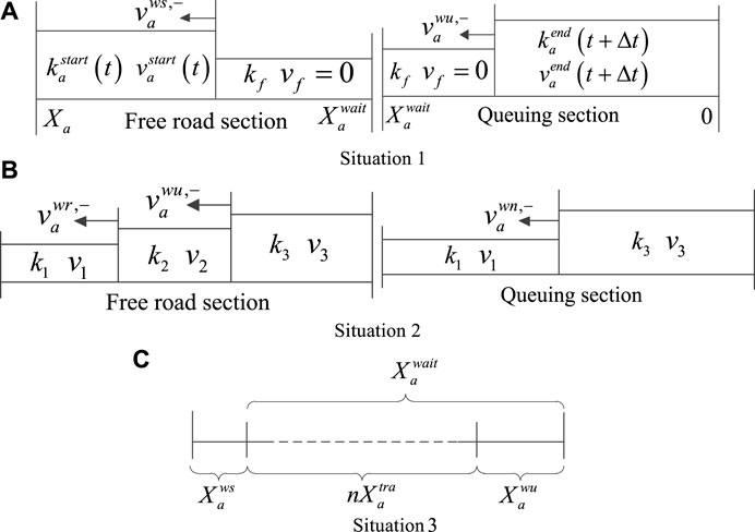
FIGURE 1. Traffic wave models in three situations. (A) Situation 1. (B) Situation 2. (C) Situation 3.

4.1.2.1 Situation 1

When a vehicle approaches a red traffic light and the traffic signal does not change before the vehicle stops, the passage time consists of two components: the first is the free driving time from entering the road section to the traffic signal change, and the second is the queuing time from the traffic signal change until the vehicle fully passes through.

The traffic flow enters the road section $a$ at an initial velocity of $v_a^{in}\left(t\right)$ and continues to travel to the queuing area where a traffic jam occurs. Assuming that the position where the vehicle stops is taken as the origin of the coordinate system, the travel time of the free driving section can be obtained based on the distance equation $x=vt$ as follows:

$t_a^{ws}=\frac{X_a^{ws}}{v_a^{ws,-}}(18)$

$X_a^{ws}=X_a-X_a^{wait}(19)$

where $v_a^{ws,-}$ is the parking wave; $X_a^{ws}$ is the driving distance from entering the road section to stopping; $X_a$ and $X_a^{wait}$ are the total length of the road section and the length of the existing queue, respectively.

After the traffic light turns green and vehicles start moving, a start-up wave is generated and the travel time is given by:

$t_a^{wu}=\frac{X_a^{wait}}{v_a^{wu,-}}(20)$

The total travel time for the road segment can be obtained as follows:

$t_a=\left\{\begin{array}{l}{t}_a^{wu}+t_{a,tra}{c}_3\le t_a^{tra},t_a^{wu}\le t_{a,grel},0<X_a^{wait}<\frac{1}{2}\overline{a}{t}_{a,tra}^2\\ t_{a,tra}{c}_3\le t_a^{tra},t_a^{wu}\le t_{a,grel},X_a^{wait}=0\end{array}\right.(21)$

where $c_3=\frac{v\pm \sqrt{v^2-2\overline{a}\left(X_a-X_a^{wait}\right)}}{\overline{a}}$; $t_{a,tra}$ is the remaining waiting time for the red light; $t_{a,grel}$ is the remaining time for the green light.

4.1.2.2 Situation 2

In the scenario where vehicles encounter a green traffic signal before they come to a complete stop at a red light, the total travel time for the road segment is the same as in situation 1. However, in the free-flowing segment, the vehicle speed decreases while the density increases, resulting in the formation of a shockwave. The velocity in front of the shockwave is given by:

$v_2=v_a^{start}\left(t\right)-\overline{a}\cdot t_{a,tra}(22)$

where $v_a^{start}\left(t\right)$ is the upstream traffic speed of section $a$ at the current time; $\overline{a}$ is the average acceleration of vehicles.

According to the Logistics speed-density model, the density $k_a^s$ of the traffic flow in front of the wavefront can be derived as follows:

$k_a^s=c_k\cdot {\log }_{{\sigma }_1}\left(\frac{c_0\cdot v_m}{v_a^s}-1\right)(23)$

${\sigma }_1={\left(\frac{c_0}{c_f}\right)}^{\frac{1}{o_f}}(24)$

where $v_a^s$ is the velocity of the vehicle flow in front of the wavefront of section $a$.

In the queuing section, if there is no queue ahead, the traffic flow produces a dissipation wave due to the increase of speed and the decrease of density, with a wave speed and travel time of:

$v_a^{wm,+}=\frac{q_a^{end}\left(t\right)-q_a^s}{k_a^s-k_a^{end}\left(t\right)}(25)$

$t_a^{wm}=\frac{X_a-v_2\cdot t_{a,tra}}{v_a^{wm,+}}(26)$

where $q_a^s$ is the traffic flow rate ahead of the shockwave.

When there is a queue ahead, the gathering wave produced by downstream traffic encounters the starting wave produced by the queued traffic upstream.

The speed of the jam wave is given by:

$v_a^{wr,-}=\frac{q_a^s\left(t\right)-q_a^{start}\left(t\right)}{k_a^s\left(t\right)-k_a^{start}\left(t\right)}(27)$

The distance equation is given by:

$X_a-\left|v_a^{wr,-}\right|\cdot t_a^{s_1}=\left|v_a^{wu,-}\right|\left(t_a^{s_1}-t_{a,tra}\right)(28)$

The encounter time between the queuing wave and the starting wave is obtained as follows:

$t_a^{s_1}=\frac{\left(X_a+\left|v_a^{wu,-}\right|\cdot t_{a,tra}\right)}{\left(\left|v_a^{wr,-}\right|+\left|v_a^{wu,-}\right|\right)}(29)$

After the meeting of the jam wave and the starting wave, the tail of the queue continues to propagate downstream with a wave speed of $v_a^{wn,-}$.

$v_a^{wn,-}=\frac{q_a^{end}\left(t\right)-q_a^{start}\left(t\right)}{k_a^{end}\left(t\right)-k_a^{start}\left(t\right)}(30)$

At this time, the distance equation is:

$X_a-\left|v_a^{wm,-}\right|\cdot \left({\tau }_a-{\tau }_a^{s_1}\right)=0(31)$

For situation 2, the total travel time $t_a$ for the two traffic conditions in the road segment $a$ is given by:

$t_a=\left\{\begin{array}{l}{t}_a^{wm}+t_{a,tra}0\le t_{a,tra}<c_3,t_a^{wm,-}\le t_{a,grel},X_a^{wait}=0\\ \frac{X_a+\left|v_a^{wu,-}\right|\cdot t_{a,tra}}{\left|v_a^{wr,-}\right|+\left|v_a^{wu,-}\right|}+\frac{X_a}{\left|v_a^{wm,-}\right|}0\le t_{a,tra}<c_3,t_a^{wm,-}\le t_{a,grel},0<X_a^{wait}\le \frac{1}{2}\overline{a}{t}_{a,tra}^2\end{array}\right.(32)$

4.1.2.3 Situation 3

When a road section becomes congested due to accidents or urban road construction, introducing new traffic flow to the section will worsen the traffic conditions, causing significantly increased travel time for upstream vehicles in the section. To ensure the stable operation of the transportation network and minimize the travel time of EVs, this paper introduces traffic flow constraints to the optimization model, and new EV traffic is not introduced to the congested sections. Therefore, situation 3 does not establish a road impedance model for the above two traffic conditions but only analyzes the traffic conditions caused by traffic signals.

The vehicle travel time consists of three parts: The first part is the travel time from when the vehicle enters the road segment to the first stop, where the traffic flow joins the queue ahead and creates a stopping wave that propagates forward at a wave speed of $v_a^{ws,-}$. The second part is the travel time from the vehicle stopping before the stop line until it passes through the intersection. Here, the traffic flow moves slowly forward due to the changing traffic signal, with a distance $X_a^{wait}$ moved of the travel distance of the last vehicle passing through the stop line in one signal cycle. The third part is the travel time from when the vehicle comes to a complete stop to when it completely passes through the stop line. Here, the traffic flow generates a starting wave that propagates forward at a wave speed of $v_a^{wu,-}$.

The total travel time $t_a$ for a road segment is given by:

$t_a=n{t}_{a,tra}+t_a^{wu}+\left\{\begin{array}{l}{t}_a^{ws}{c}_3\le t_{a,tra},t_a^{wu}\le t_{a,grel},\frac{1}{2}\overline{a}{t}_{a,tra}^2\le X_a^{wait}\\ t_a^{s_1}0\le t_{a,tra}<c_3,t_a^{wm,-}\le t_{a,grel},\frac{1}{2}\overline{a}{t}_{a,tra}^2\le X_a^{wait}\end{array}\right.(33)$

$\left\{\begin{array}{l}{t}_a^{ws}=\frac{X_a-X_a^{wait}}{v_a^{ws,-}}\\ t_a^{s_1}=\frac{\left(X_a+\left|v_a^{wu,-}\right|\cdot t_a^{tra}\right)}{\left(\left|v_a^{wr,-}\right|+\left|v_a^{wu,-}\right|\right)}\\ X_a^{tra}=\frac{1}{2}\overline{a}{\left(t_{a,tra}\right)}^2\\ t_a^{wu}=\frac{X_a^{wait}-n{X}_a^{tra}}{v_a^{wu,-}}\\ n=\left[\frac{X_a^{wait}}{X_a^{tra}}\right]\end{array}\right.(34)$

where $w_{ij}$ is the impedance value of the road segment; is the rounding function.

This study considers the scenario where vehicles encounter a green light. It is assumed that, in the absence of a queue, vehicles exit the section at a constant speed of 60 km/h. However, in the presence of a queue, the calculation is performed based on situation 2.

4.2 Path planning model

4.2.1 The objective function

The objective function is established from two aspects: the benefits of the vehicle owners and the coupled network state.

$F=\frac{{\gamma }_1}{\min \left(C^{E{V}^{\prime }}\right)}{C}^{EV}\left(t\right)+\frac{{\gamma }_2}{\min \left(T^{E{V}^{\prime }}\right)}{T}^{EV}\left(t\right)+\frac{{\gamma }_3}{\min \left(S^{E{V}^{\prime }}\right)}{S}^{EV}\left(t\right)+\frac{{\gamma }_4}{\min \left(R^{E{V}^{\prime }}\right)}{R}^{EV}\left(t\right)(35)$

where $C^{EV}$ and $T^{EV}$ are the optimization objectives for EV charging; $S^{EV}$ is the optimization objective for power grid operation; $R^{EV}$ is the optimization objective for traffic network state; ${\gamma }_1$, ${\gamma }_2$, ${\gamma }_3$ and ${\gamma }_4$ are the weighting coefficients of the objectives.

4.2.1.1 The cost of an EV trip

Considering the maximization of the car owner’s interests, the optimization is carried out by minimizing the sum of the economic and time costs. The model is as follows:

$\left\{\begin{array}{l}{C}^{EV}\left(t\right)=C^{route}\left(t\right)+C^{ch\mathit{arg}e}\left(t\right)\\ T^{EV}\left(t\right)=T_{drive}\left(t\right)+T_{char}\left(t\right)\end{array}\right.(36)$

$\left\{\begin{array}{l}{C}_{ch\mathit{arg}e}\left(t\right)=p\times q_{char,c}\left(t\right)\\ C_{route}\left(t\right)=q^{EV}\cdot \overline{p}\cdot {\displaystyle \sum }_{i,j\in N}{l}_{ij}\left(t\right)\end{array}\right.(37)$

$\left\{\begin{array}{l}{T}_{drive}\left(t\right)={\displaystyle \sum }_{i,j\in N}{x}_{ij}{T}_{ij}\left(t\right){\rho }_{ij},{\chi }_i={\displaystyle \sum }_{i,j\in V^T}{L}_{ij}^R{e}^{\frac{20T_{ij}\left(t\right)}{l_{ij}}}\\ T_{cha}\left(t\right)=T_{wait,c}^{char}\left(t\right)+T_{char,c}^{char}\left(t\right)\end{array}\right.(38)$

where $C^{EV}\left(t\right)$ and $T^{EV}\left(t\right)$ are the economic cost and time cost, respectively; $C^{route}\left(t\right)$ and $C^{ch\mathit{arg}e}\left(t\right)$ are the driving cost and charging cost for the EV; $T_{drive}\left(t\right)$ and $T_{char}\left(t\right)$ are the driving time and charging time for the EV; $p$ is the charging price; $q_{char,c}\left(t\right)$ is the charging amount for the $c$-th EV; $q^{EV}$ is the energy consumption per 100 km for the EV; $N$ is the set of all nodes in the road network and service stations; $\overline{p}$ is the average electricity cost for the EV; $x_{ij}$ is the path selection variable; $T_{ij}\left(t\right)$ is the time for a vehicle to pass through road segment $ij$ at the current time; ${\rho }_{ij}$ is the congestion penalty coefficient for the road segment; $T_{wait,c}^{char}\left(t\right)$ and $T_{wait,c}^{swap}\left(t\right)$ are the waiting time for the vehicle to charge and replace the battery at the service station, respectively; $L_{ij}^R$ is the grade coefficient of road $ij$, which is set to 1.2.

4.2.1.2 The state of the power distribution network

The evaluation of the distribution network status is based on ensuring the safe operation of the system. To assess the status of the distribution network, this model employs the voltage deviation index and branch loss index. The optimization objective is selected as the load of the charging station that is connected to the distribution network.

$S^{EV}\left(t\right)={\displaystyle \sum _{b=1}^{n_{CS}}}{S}_b^{EV}\left(t\right)={\mathrm{\Gamma }}_d^{loss}\left(t\right)\cdot {\mathrm{\Gamma }}_d^U\left(t\right)\cdot \frac{1}{P_b^{CS}\left(t+1\right)}(39)$

$\left\{\begin{array}{l}{\mathrm{\Gamma }}_d^U\left(t\right)=\frac{U_{\mathrm{d},\max }-U_d\left(t\right)}{U_{\mathrm{d},\max }}\\ {\mathrm{\Gamma }}_d^{loss}\left(t\right)=\frac{P_e^2\left(t\right)+Q_e^2\left(t\right)}{U_d^2\left(t\right)\cdot P_e\left(t\right)}{R}_e\end{array}\right.(40)$

where ${\mathrm{\Gamma }}_i^{loss}\left(t\right)$ and ${\mathrm{\Gamma }}_i^U\left(t\right)$ are the voltage deviation and branch loss index of node $d$, respectively; $P_b^{CS}\left(t+1\right)$ is the load connection capacity of the charging station at the next time; $U_d\left(t\right)$ is the voltage magnitude of node $d$ at the current time; $U_{d,\max }$ is the voltage upper limit of node $d$; $e$ is the branch connected to node $d$; $P_e^2\left(t\right)$ and $Q_e^2\left(t\right)$ are the active and reactive power of branch $e$ at the current time, respectively; $R_e$ is the equivalent resistance value of branch $e$.

4.2.1.3 The state of the transportation network

The risk propagation path and fault probability model established in (Huang et al., 2019) is used to construct a measurement index. The specific model is as follows:

$P\left(q_a\right)=\left\{\begin{array}{l}0,q_a\le Q_a\\ \frac{\left(q_a-Q_a\right)}{\left(1+\gamma \right)Q_a}-Q_a{Q}_a\le q_a\le \left(1+\gamma \right)Q_a\\ 1,\left(1+\gamma \right)Q_a\le q_a\end{array}\right.(41)$

$R^{EV}={\displaystyle \sum }_{a\in L_c}P\left(q_a\right)\times W_a(42)$

where $P\left(q_{ij}\right)$ is the probability of failure for road segment $a$ with initial flow rate of $q_{ij}$; $q_a$ is the upper limit of the load capacity of road segment $a$; $Q_a$ is the importance of road segment $a$, which is the product of the sum of the importance of the two endpoints of road segment $a$ and the node efficiency; $\gamma$ is the fault probability adjustment parameter, which is set to 1; $L_c$ is the set of road segments passed by the $c$-th EV; $W_a$ is the risk path propagation weight of the road segment, which is the product of the degrees of the two end nodes.

4.2.2 Constraints

4.2.2.1 The operation constraints of charging stations and distribution network

To ensure the safe operation of the charging station and the distribution network, the following constraints are introduced: charging station load constraints, power flow constraints, and voltage constraints on the lines.

$P_{d,\max }^{DN}\left(t\right)\ge P_b^{ES}\left(t\right)(43)$

$P_e^l\left(t\right)\le P_{e,\max }^l(44)$

$U_{d,\min }\left(t\right)\le U_d\left(t\right)\le U_{d,\max }\left(t\right)(45)$

where $P_{d,\max }^{DN}\left(t\right)$ is the rated charging capacity of node $d$ in the power distribution network at the current time; $P_b^{ES}\left(t\right)$ is the charging load of charging station $b$ at the current time; $P_e^l\left(t\right)$ and $P_{e,\max }^l$ are respectively the transmission capacity and the maximum transmission capacity of line $e$ in the power distribution network at the current time; $U_d\left(t\right)$ is the voltage level of node $d$ in the power distribution network at the current time; $U_{d,\min }\left(t\right)$ and $U_{d,\max }\left(t\right)$ respectively are the upper and lower voltage limits of node $d$ in the power distribution network.

4.2.2.2 The operation constraints of the transportation network

In China, the evaluation standard for urban traffic operation defines “moderate congestion” as the traffic state of a road segment (Ministry of Transport of the People’s Republic of China, 2016). However, due to the longer travel time on such road segments, EVs may not be able to complete the charging process and reach their destinations within the planned time, which could result in path search failure.

To prevent the congested road segments from deteriorating as a result of the introduction of EV traffic and to ensure that at least one feasible path can be found, the following traffic constraints are established:

$\left\{\begin{array}{l}{\overline{v}}_a\left(t\right)\ge 20\%v_0\\ {\overline{v}}_a\left(t\right)=v_0\cdot \left(1-\frac{{\overline{o}}_a\left(t\right)}{o_f}\right)\end{array}\right.(46)$

where ${\overline{v}}_a\left(t\right)$ is the average travel speed of segment $a$.

4.2.2.3 Solution algorithm

In this study, the A* algorithm is used to solve the proposed path planning problem because it determines the search direction based on the estimated path cost, thus avoiding searching all directions and ensuring search efficiency.

5 Case study

5.1 Example parameters

This study analyzes and verifies a 90-node traffic system and three IEEE33-node power systems (Xing et al., 2020) as examples. The road network consists of 90 road nodes, 13 charging station nodes, and 147 road segments, covering approximately 22.4 km in length and 49 km² in area. The basic data for the coupled network and charging stations can be found in (Xing et al., 2020). The study specifically analyzes the operation of the distribution network and transportation network during the 16:00–17:00 period, with three fault scenarios set.

Scenario 1. The 4th node of the 2nd distribution network is faulty, and the 5th charging station terminates service.

Scenario 2. Building on Scenario 1, the 26th node of the 1st distribution network is also faulty, and the 12th charging station terminates service.

Scenario 3. Building on Scenarios 1 and 2, the 4th node of the 1st distribution network is also faulty, and the 1st charging station terminates service.

5.2 Impedance analysis of roads based on traffic wave theory

To verify the accuracy of the proposed impedance model in this paper, the travel time of the road segment is used as the output of the model. The results of the proposed model are compared and analyzed with those obtained from the traditional BPR impedance function method in terms of T/T0 calculation, travel time calculation, and error analysis. The error analysis is shown in Table 1, which uses the mean absolute error, the mean absolute percentage error, and the root mean square error for the error analysis. The specific calculation formulas can be found in the literature (Wang et al., 2021). The results of relative error calculation are shown in Figure 2.

TABLE 1

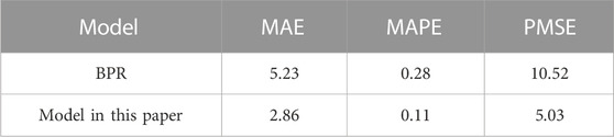
TABLE 1. Comparison of calculation results between improved model and classic model.

FIGURE 2

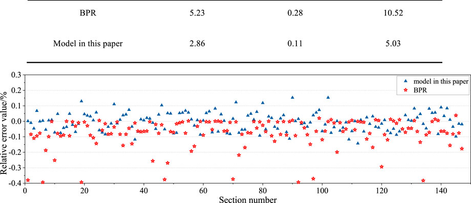
FIGURE 2. Comparison of relative error value calculation results between im-proved model and classic BPR model.

Figure 2A compares the impedance values of 147 roads in the traffic network, while Figure 2B presents the relative error values. In the results of this study’s model calculation, 57.82% of the road segments have a relative error of less than 5%, while 37.41% have an error between 5% and 10%, and only 4.77% of the road segments have an error greater than 10%. Among them, 43 road segments have a travel time of less than 1 min. Of these, 38 road segments have a relative error between 5% and 10%, accounting for 88.37% of the total number of road segments in this part. There are 77 road segments with a travel time exceeding 3 min, accounting for 52.38% of the total number of road segments. Among them, 65 road segments have a relative error of less than 5%, accounting for 84.42% of the total number of road segments in this part. There are 11 road segments with a travel time exceeding 5 min. Among them, the relative error values for roads 1, 5, 59, 85, 95, 105, and 130 are less than 1%, with a maximum of 1.12%. Compared with the BPR model, the proposed model’s relative errors in oversaturated road sections with travel times over 5 min are all below 5%, while those of the BPR model are close to 40%. In saturated road sections 7, 33, 52, 57, 105, 117, and 147, the proposed model’s errors are all below 5.19%, while those of the BPR model range from 15% to 20%. In low-saturated road sections with travel times less than 5 min, only eight road sections have errors exceeding 10% in the proposed model. Among them, road sections 19, 71, 90, and 102 have relatively larger errors of 19.32%, 14.88%, 15.41%, and 16.16%, respectively, while the remaining four road sections have errors close to 10%. Therefore, in low-saturation road segments, the proposed model in this paper meets the accuracy requirements. In saturated and oversaturated road segments, the calculated results of the classical BPR model have a large deviation from the observed values, while the proposed model in this paper has smaller errors and higher fitting accuracy.

To demonstrate the advantages and disadvantages of different methods in calculating results, a detailed display of the travel time calculation results for the time-occupancy ratio road impedance model, the actual observed results, and the classic BPR road impedance model is presented in Figure 3. A comparison of the T/T0 calculation results for the time-occupancy ratio road impedance model, the actual observed results and the T/T0 calculation results for the BPR classic road impedance function model is shown in Figure 4.

FIGURE 3

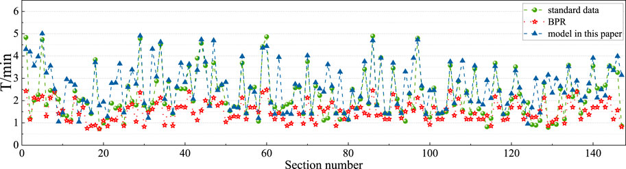
FIGURE 3. Comparison of road impedance value calculation results between im-proved model and classic BPR model.

FIGURE 4

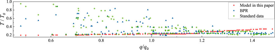
FIGURE 4. The comparison of the T/T_f calculation results between the model in this paper and the classical impedance model.

As is shown in Figure 3 that compared to the actual observed results, the calculated values of the BPR model are smaller, which is equivalent to two-thirds of the actual observed data, while the proposed model in this paper has a higher fitting accuracy in calculating travel time results. From Figure 4, it can be seen that the calculated results of the classical BPR impedance model show a monotonically increasing state, which does not match the actual situation. Therefore, the proposed model in this paper can more accurately calculate the travel time of road segments in the surveyed area.

5.3 Analysis of EV charging behavior and coupled network operation status

5.3.1 Analysis of EV charging paths

This section analyzes four EVs (No. 2, 5, 7, and 9) located on congested and uncongested road segments.

5.3.1.1 Scenario 1: Failure of charging station 5

In Scenario 1, two sets of weight coefficients for the objective function are used to plan the charging path, corresponding to the disordered charging and ordered charging strategies. To ensure successful path searching under the disordered charging strategy, the constraints on traffic network operation are relaxed. The weight coefficients are determined using the deviation sorting method established in (Li et al., 2022). The path planning results are presented in Table 2 and Table 3.

TABLE 2

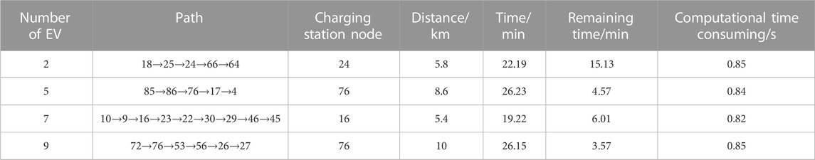
TABLE 2. Disordered charging route planning results of EV.

TABLE 3

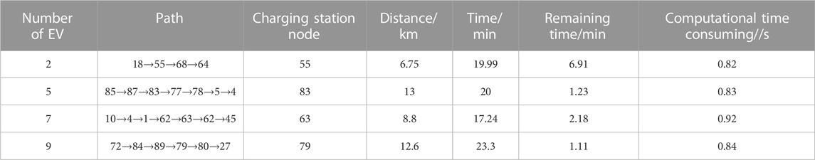
TABLE 3. Coordinated charging route planning results of EV.

Under the disordered strategy, the total driving distance of EVs is shorter. However, nearby charging causes traffic congestion, leading to a large increase in the total travel time due to the large number of queued vehicles. Taking EV 2 as an example, its target charging station is close to the fault coupling point, resulting in a significantly longer queue time than other EVs, with a total travel time of 15.13 min, including a charging queue time of 11.2 min, which is 4.46 times higher than the daily average value. The total travel time is 28.66% higher than that of the ordered strategy.

Under the ordered strategy, the journey delay time is reduced to 2.19 min, and the queue time is only 5.11 min. Although the total delay time is still higher than the daily average value due to the peak charging period, the operating parameters of the distribution and traffic networks do not exceed the threshold, ensuring the safe and stable operation of the coupled network under the fault condition.

5.3.1.2 Scenario 2: Failure of charging stations 5 and 12

Taking EV 9 as an example, in comparison to Scenario 1, the EV selects the “detour” option with better traffic conditions. Although the distance increases by 3.17%, the driving time reduces by 0.81 min. As the number of malfunctioning charging stations increases, the charging waiting time increases by 1.66 min, and the total travel time increases by 0.85 min, with a user satisfaction rate of 87.78%. If an unordered charging strategy is implemented, the driver still selects charging station 76 due to a deviation in the perception of road network status. The total travel time is 4.49 min, which is 2.37 times longer than the ordered strategy. The charging waiting time is 3.21 min, which is 88.82% longer than the ordered strategy. Although the total stop time is still acceptable, the road section is slightly congested due to two malfunctioning nodes, and the driver satisfaction rate decreases to 84.7%.

5.3.1.3 Scenario 3: Failure of charging stations 1, 5, and 12

Taking EV 9 as an example, Table 4 shows the planning results. Under the unordered charging strategy, the roadside stop time is 3.09 min, which is 66.49% longer than the ordered strategy. The waiting time is 4.8 min, which is 4.36 times longer than the ordered strategy. As the scope of malfunctions expands, more than 20% of road sections become oversaturated, resulting in a significant increase in total travel time for EVs. However, the waiting time does not exceed 10 min, and the satisfaction rate remains above 80%. Therefore, the path planning scheme is still feasible.

TABLE 4

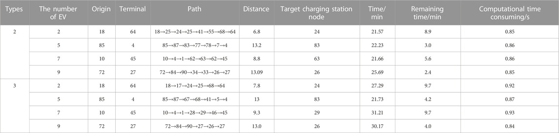
TABLE 4. Search process of EV in scene2.

5.3.2 The analysis of the impact on the distribution network side

Figure 5 shows the topology of the distribution network after scheduling, and Figure 6 depicts the load variations of the charging stations. The upper and lower surfaces of the surface plots correspond to the load variations after adopting the uncoordinated and coordinated charging strategies, respectively.

FIGURE 5

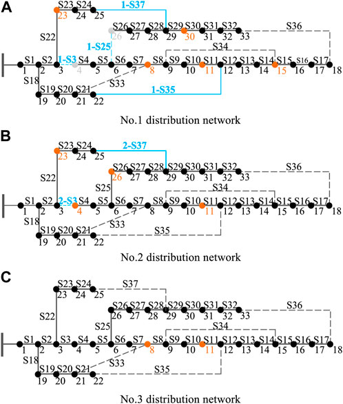
FIGURE 5. Topological structure of distribution network. (A) No.1 distribution network. (B) No.2 distribution network. (C) No.3 distribution network.

FIGURE 6

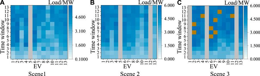
FIGURE 6. Charging station load. (A) Scene1 (B) Scene 2 (C) Scene 3.

In Scenario 1, branch 2-S3 is faulted, triggering the closure of contact switch 2-S37 and restoring the system connectivity. The minimum node voltage of the system is 11.75 kV, and the maximum power transmission capacity of the line is 7.41 MW, which exceeds the threshold by 5.86%. To address this issue, third-level loads 10, 14, 19, and 21 of the No. 1 distribution network and third-level loads 9, 27, and 29 of the No. 2 distribution network are disconnected.

In Scenario 2, branch 1-S25 is added as a fault, triggering contact switch 1-S37. In Scenario 3, branch 1-S3 is added as a fault, triggering contact switch 1-S35. The minimum system voltages are 11.962 kV and 12.159 kV, respectively, and the line transmission powers are both less than 7 MW, with no line overload or voltage violations observed. The scheduling process is completed.

In Scenario 1, after adopting the uncoordinated strategy, charging stations 1, 2, 6, and 7 exceed the threshold in the 6th time window, with loads of 6.7687 MW, 6.8642 MW, 6.369 MW, and 6.5315 MW, respectively. At this time, the minimum loads of the four stations are 2.76 MW, 2.98 MW, 2.62 MW, and 2.32 MW, respectively, with significant differences in load peaks and valleys. After adopting the coordinated strategy, only charging station 6 approaches the threshold in the 10th time window, with a load of 5.98 MW, and the minimum load increases to 3.1438 MW. The peak loads of the other charging stations are all less than 4.2 MW, with a minimum load of 3.221 MW. All charging station loads decrease to within the threshold, and the peak-to-valley difference decreases, which is beneficial for the stable operation of the charging stations.

In Scenario 2, charging stations 1, 4, and 6 have peak loads in the 8th and 9th time windows, with loads of 5.7546 MW, 5.7981 MW, and 5.6495 MW, respectively. In Scenario 3, charging stations 2, 6, 7, 8, and 11 approach the threshold in the 6th to 12th time windows, with charging station 7 having a peak load of 5.998 MW in the 10th time window.

Figure 7 illustrates the voltage variation of the nodes for the unordered and ordered charging strategies. The voltage deviation rate of nodes 14–18 exceeds the limit under the unordered strategy, which poses a threat to the safe operation of the distribution network. However, under the ordered strategy, the average voltage deviation rates of the distribution network for the three scenarios are 3.03%, 3.23%, and 3.53%, respectively, all of which are within the deviation limit of 7%. Therefore, the planning scheme can guarantee the safe operation of the distribution network.

FIGURE 7

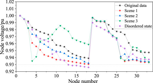
FIGURE 7. Node voltage of distribution network.

5.3.3 Traffic network impact analysis

To describe the level of congestion, the TTI index is used as the evaluation indicator in this section, and the conversion relationship is shown in Table 5. In Scenario 1, after adopting the disordered charging strategy, 21.77% of the road segments were in a congested state, with a maximum TTI value of 2.02. After adopting the ordered charging strategy, even during the peak charging period from 16:20 to 16:35, only 11 road segments experienced slight congestion, accounting for 7.48% of the total, and the maximum TTI value was only 1.64. Although there are still a few lightly congested road segments, the traffic flow distribution is more even, which helps alleviate traffic congestion.

TABLE 5

TABLE 5. Relationship between TTI and traffic condition grade transition.

Figure 8 shows the distribution of road traffic in the three scenarios. In Scenario 2, 27 road sections experienced minor congestion between 16:20 and 16:40, accounting for 11.2% of the total. The average TTI was 1.41, with a maximum of 1.7. In Scenario 3, 53 road sections experienced congestion between 16:15 and 16:55, accounting for 36.1% of the total. The average TTI was 1.55, with a maximum of 1.812. As the fault range expanded, the number of congested roads increased significantly; however, the overall traffic flow remained relatively smooth. Therefore, the planning scheme can ensure the safe and continuous operation of the traffic network.

FIGURE 8

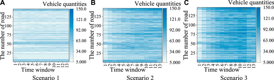
FIGURE 8. Number of vehicles in three scenarios. (A) Scenario 1 (B) Scenario 2 (C) Scenario 3.

5.4 Analysis of EV charging behavior and coupled network operation status

(1) The satisfaction index is used to evaluate the planning results under different weight ratios, and the impact of the preferences of drivers on path planning is quantitatively analyzed. The specific model is as follows:

${\sigma }_c=\frac{1}{2}{\displaystyle \sum }_{i\in V^T}\left(\frac{C_i^{EV}-C_{i,\min }^{EV}}{C_{i,\min }^{EV}}+\frac{T_i^{EV}-T_{i,\min }^{EV}}{T_{i,\min }^{EV}}\right)(47)$

where $C_i^{EV}$ and $T_i^{EV}$ are the economic and time costs of passing through the road nodes, respectively; $C_{i,\min }^{EV}$ and $T_{i,\min }^{EV}$ are the minimum values of the economic and time costs of passing through the road nodes respectively.

(2) This section uses the ratio of access capacity to transmission power to quantify the operating status of the charging station and uses satisfaction indicators to measure the effect of changes in the operating status of the charging station on the path planning result. The specific model is as follows:

${\theta }_b^{CS}\left(t\right)=\frac{P_b^{CS}\left(t\right)}{P_i^{load}\left(t\right)}\times 100\%(48)$

where ${\theta }_b^{CS}\left(t\right)$ is the utilization rate of charging station $b$ at the current time; $P_b^{CS}\left(t\right)$ is the access capacity of charging station $b$ at the current time; $P_i^{load}\left(t\right)$ is the transmission power of the distribution network node connected to charging station $b$.

(3) This section measures the importance of a coupling node by the proportion of lost capacity. The model is defined as follows:

${\zeta }_b^{ca}\left(t\right)=\frac{P_f^{CS}\cdot {\theta }_b^{CS}\left(t\right)}{{\displaystyle \sum _{b=1}^{n_{CS}}}{P}_b^{CS}}\times 100\%(49)$

where ${\zeta }^{ca}\left(t\right)$ is the percentage of the capacity loss for the current time of charging station $b$; $P_f^{CS}$ is the rated capacity of the failed charging station; ${\theta }_b^{CS}\left(t\right)$ is the utilization rate of charging station $b$ at the current time; $P_b^{CS}$ is the rated capacity of charging station $b$.

Taking EV No.9 as an example, the satisfaction results are shown in Figure 9.

FIGURE 9

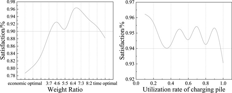
FIGURE 9. Satisfaction calculation results.

5.4.1 Impact of objective function weight on planning results

As shown in Figure 9, the satisfaction degree of the path planning results is all above 75%. Among them, when the weight ratio exceeds 3:7, the satisfaction degree exceeds 90%. This indicates that under the fault state, the travel time has a greater impact on the planning results, and the car owners tend to choose the path plan with the shortest travel time.

5.4.2 Impact of charging station operational status on planning results

When the utilization rate of charging piles is less than 1, the satisfaction of car owners is above 94%. When the utilization rate reaches 1, the satisfaction drops to 93.1%. This indicates that in a fault state, driving time has a greater impact on the planning results, when there are available charging spots in the charging station, the satisfaction is higher, and the impact of the charging station’s operational status on the planning results is smaller. When there is a queue in the charging station, the satisfaction of car owners is affected by the waiting time, and the impact of operational status of the charging station on the planning results deepens.

5.4.3 Impact of the importance of coupling nodes on the scope of fault propagation

To compare the propagation range of coupling failures in the transportation network caused by the power outage of coupling nodes with different importance levels, this section introduces two new scenarios: Scenario 4 and Scenario 5.

(1) Scenario 1: Node 4 in distribution network 2 fails, and charging station 5 connected to this node terminates service, with a power outage capacity ratio of 7.14%.

(2) Scenario 4: Node 15 in distribution network 1 fails, and charging station 4 connected to this node terminates service, with a power outage capacity ratio of 6.57%.

(3) Scenario 5: Node 11 in distribution network 3 fails, and charging station 10 connected to this node terminates service, with a power outage capacity ratio of 2.7%.

The number of road vehicles in Scenario 4 and Scenario 5 are shown in Figure 10. Comparing Scenario 1 and scenario 5, it can be observed that when a heavily affected charging station fails, there are significantly more congested road sections than when a lightly affected charging station fails, indicating a more pronounced impact on the transportation network. Comparing Scenario 1 and scenario 4, it can be seen that station 5 can distribute the affected charging flows to nearby stations such as stations 1, 2, 4, and 6, as well as the more remote station 10. Although the moderately congested road sections are more numerous than in scenario 4, the flow peak-to-valley ratio is smaller, indicating a more even distribution.

FIGURE 10

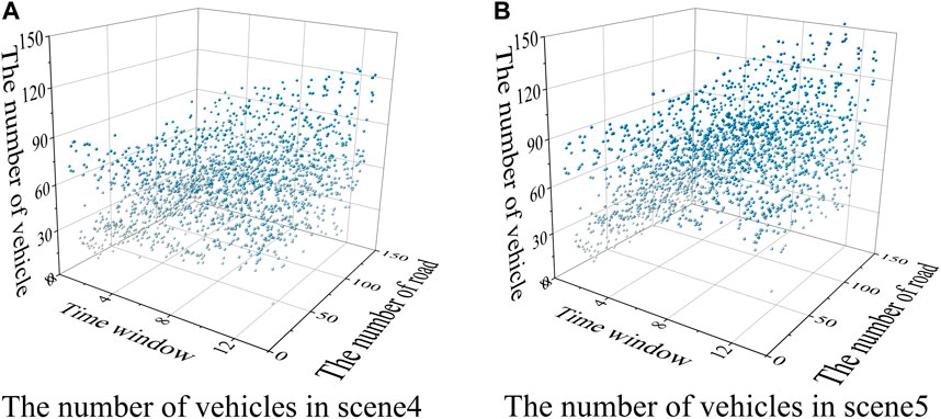
FIGURE 10. The number of vehicles in scene 4 and scene 5. (A) Scene4 (B) Scene5.

Therefore, after a fault occurs, the overall state of the transportation network is affected not only by the capacity of the failed node, but also by the geographical location of the failed node within the transportation network and the distribution of nearby charging stations.

5.5 Impact of charging station load weighting coefficients on path planning results

When setting the load weighting coefficient of all charging station nodes in Scenario 1 to 0.1, the scheduling result is still the closure triggered by the connection switch 2-S37, and the loads of third-level loads 10, 14, 19, 21 in the first distribution network, loads 9, 27, 29 in the second distribution network, and loads of charging stations 4 and 7 are shed. The proportion of slightly congested road segments in the traffic network are 7.8%, 11.2%, and 36.1%, respectively, with no moderately congested road segments.

When the load weighting factors of all the charging station nodes in Scenario 1 are set to 0.01, the dispatching result is changed to the closure of the switch 2-S35, and the third-level loads 3, 10, 19, and 21 in the 1st distribution network and the loads of charging stations 1, 2, 5, 11, and 12 in the 2nd distribution network are shed, as well as loads 3, 9, 22, 27, 29, and 30 in the 2nd distribution network. At this point, the proportion of lightly congested road sections is 38.46%, with no moderately congested road sections. Charging stations 3, 6, 7, 9, and 13 are close to their threshold loads in the 4th to 12th time windows, and EV route planning fails for stations 5, 7, and 10. The distribution of road traffic flow is shown in Figure 11. If the operating constraints of the traffic network are released, the proportion of lightly congested road sections would reach 49.63%, with road sections 63, 75, 98, 117, 130, 131, and 135 becoming moderately congested, accounting for 4.76% of the total, and the maximum TTI value reaching 2.08.

FIGURE 11

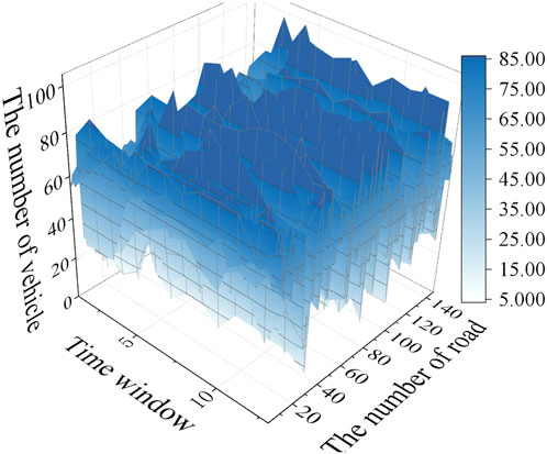
FIGURE 11. The number of vehicles when the weight coefficient is 0.01.

5.6 Output performance of different solution algorithms

Currently, commonly used global path planning algorithms include A* algorithm and Dijkstra algorithm. The Dijkstra algorithm selects the shortest edge from the previous node as the search path, which may traverse the entire network before reaching the target node, and cannot guarantee search efficiency. The proposed path planning solution in this paper continuously updates the planning results based on real-time network information within a short period of time, and it is necessary to ensure that the search time is less than the update time. In order to verify the impact of different algorithms on the solving speed and performance, a planning function with the shortest distance as the goal is constructed, and two algorithms are used to solve the path planning model that needs to be charged, and the simulation results are obtained as shown in Table 6 and Figure 12.

TABLE 6

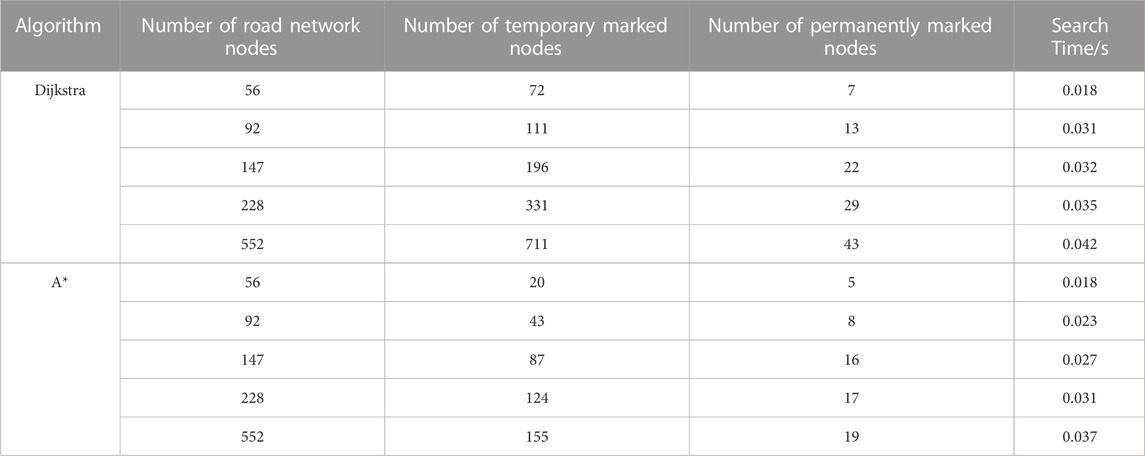
TABLE 6. Comparison of different algorithms.

FIGURE 12

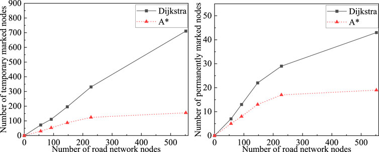
FIGURE 12. Comparison of the results of different algorithms for solving parameters.

In a small area of road network, the performance of Dijkstra algorithm and A* algorithm for solving path planning problems is similar. However, as the size of the road network increases, A* algorithm has advantages over Dijkstra algorithm in terms of time complexity and space complexity. Experimental results show that in a large area of road network, the number of nodes marked by Dijkstra algorithm exceeds the number of nodes in the network, with the maximum number of marked nodes reaching twice the number of nodes in the network. Therefore, A* algorithm is more suitable for the path planning model proposed in this paper.

6 Conclusion

In response to the uncontrolled charging behavior of EVs and its impact on the coupled network after a distribution network failure, this study considers the propagation path of coupled faults and establishes an EV path planning model with the objectives of minimizing EV travel costs, optimizing the distribution network, and traffic operation status. To accurately calculate the travel time of vehicles on road segments, a road impedance model is established based on the traffic wave theory and Logistics speed-density model, considering three traffic conditions. The conclusions are as follows.

1) During high load peak periods, midstream road segments experience severe density fluctuations. Analyzing the evolution of traffic flow under multi-time scales from the perspective of macro traffic flow fluctuations is more in line with the actual situation of the traffic network.

2) Under the influence of coupled faults, downstream queue length and incoming traffic at upstream intersections increase significantly, resulting in complex traffic conditions in the midstream. The time-time occupancy rate model established in this study can accurately calculate the travel time of vehicles based on the fluctuation of traffic flow under different spatiotemporal states.

3) Based on the background of coupled fault propagation between the two networks, the optimal path planning solution proposed in this paper can significantly reduce the travel time of EVs, rationally allocate EV traffic, reduce the peak-to-valley difference of the distribution network load, block the further propagation of coupled faults, and ensure the safe and stable operation of the distribution network and traffic network after the failure.

Data availability statement

The original contributions presented in the study are included in the article/Supplementary Material, further inquiries can be directed to the corresponding author.

Author contributions

All authors listed have made a substantial, direct, and intellectual contribution to the work and approved it for publication.

Funding

This work was supported by the National Natural Science Foundation of China, grant number U1936213.

Conflict of interest

The authors declare that the research was conducted in the absence of any commercial or financial relationships that could be construed as a potential conflict of interest.

Publisher’s note

All claims expressed in this article are solely those of the authors and do not necessarily represent those of their affiliated organizations, or those of the publisher, the editors and the reviewers. Any product that may be evaluated in this article, or claim that may be made by its manufacturer, is not guaranteed or endorsed by the publisher.

References

Betancur, D., Duarte, L. F., Revollo, J., Restrepo, C., Díez, A. E., Isaac, I. A., et al. (2021). Methodology to evaluate the impact of electric vehicles on electrical networks using Monte Carlo. Energies 14, 1300. doi:10.3390/en14051300

CrossRef Full Text | Google Scholar

Cai, J. P., Chen, D. W., Jiang, S. X., and Pan, W. J. (2020). Dynamic-area-based shortest-path algorithm for intelligent charging guidance of electric vehicles. Sustainability 12 (18), 7343. doi:10.3390/su12187343

CrossRef Full Text | Google Scholar

Ding, T., Wang, Z., Jia, W., Chen, B., Chen, C. M., and Shahidehpour, M. (2020). Multiperiod distribution system restoration with routing repair crews, mobile electric vehicles, and soft-open-point networked microgrids. IEEE Trans. Smart Grid 11, 4795–4808. doi:10.1109/TSG.2020.3001952

CrossRef Full Text | Google Scholar

Evers, E. R. K., Imas, A., and Kang, C. (2022). On the role of similarity in mental accounting and hedonic editing. Psychol. Rev. 129 (4), 777–789. doi:10.1037/rev0000325

PubMed Abstract | CrossRef Full Text | Google Scholar

Feizizadeh, B., Omarzadeh, D., Sharifi, A., Rahmani, A., Lakes, T., and Blaschke, T. (2022). A GIS-based spatiotemporal modelling of urban traffic accidents in tabriz city during the COVID-19 pandemic. Sustainability 14, 7468. doi:10.3390/su14127468

CrossRef Full Text | Google Scholar

Huang, G., Chen, B., Xiao, L., Ruan, Y., and Zhang, G. (2019). Cascading Fault analysis and control strategy for computer numerical control machine tools based on meta action. IEEE Access 7, 91202–91215. doi:10.1109/ACCESS.2019.2927008

CrossRef Full Text | Google Scholar

Jiang, G. Y., Li, J. W., and Zhang, C. Q. (2010). Modified bpr functions for travel time estimation of urban arterial road segment. J. Southwest Jiaot. Univ. 45 (1), 124–129. doi:10.3969/j.issn.0258-2724.2010.01.021

CrossRef Full Text | Google Scholar

Li, W., Wang, J., Bai, H., Wang, S., and Ma, C. (2020). An accident induction and evacuation system considering the mixing rate of the large vehicles under the freeway network. China J. Highw. Transp. 33, 275–284. doi:10.19721/1001-7372.2020.11.025

CrossRef Full Text | Google Scholar

Li, Y., Li, O., Wu, F., Shi, L., Ma, S., and Zhou, B. (2022). Coordinated multi-objective capacity optimization of wind-photovoltaic-pumped storage hybrid system. Energy Rep. 8 (13), 1303–1310. doi:10.1016/j.egyr.2022.08.160

CrossRef Full Text | Google Scholar

Liu, J., Zhang, H., Liu, A., Cao, S., Li, L., Wang, Y., et al. (2022). A unified global genotyping framework of dengue virus serotype-1 for a stratified coordinated surveillance strategy of dengue epidemics. Automation Electr. Power Syst. 46, 107–118. doi:10.1186/s40249-022-01024-5

CrossRef Full Text | Google Scholar

Ma, X. L., Ma, D. F., Wang, D. H., and Lin, S. (2015). Modeling of speed-density relationship in traffic flow based on logistic curve. China J. Highw. Transp. 28 (4), 94–100. doi:10.19721/j.cnki.1001-7372.2015.04.012

CrossRef Full Text | Google Scholar

Ministry of Transport of the People’s Republic of China (2016). Specification for urban traffic performance evaluation: GB/T 33171—2016. Beijing: General Administration of Quality Supervision, Inspection and Quarantine of the people’s Republic of China.

Google Scholar

Su, S., Wei, C., Chen, Q., Li, Z., and Xia, M. (2022). S patio-temporal hierarchical scheduling for electric vehicle energy considering the assistance of urban road repair to critical loads restoration. Automation Electr. Power Syst. 46, 140–150. doi:10.7500/AEPS20211223002

CrossRef Full Text | Google Scholar

Wang, F., Xu, W., and Onega, T. (2021). Network optimization approach to delineating health care service areas: Spatially constrained louvain and leiden algorithms. J. Zhejiang Univ. Eng. Sci. 55 (6), 1065–1081. doi:10.1111/tgis.12722

CrossRef Full Text | Google Scholar

Wu, F. Z., Yang, J., Lin, Y. J., Xu, J., and Sun, Y. Z. (2020). Research on spatiotemporal behavior of electric vehicles considering the users’ bounded rationality. Trans. China Electrotech. Soc. 35 (7), 1563–1574. doi:10.19595/j.cnki.1000-6753.tces.190475

CrossRef Full Text | Google Scholar

Xing, Q., Chen, Z., Leng, Z., Liu, Y., and Liu, Y. (2020). Route planning and charging navigation strategy for electric vehicles based on real-time traffic information. Proc. CSEE 40 (2), 534–550. doi:10.13334/j.0258-8013.pcsee.182001

CrossRef Full Text | Google Scholar

Yang, Y., Zhang, T. Y., Zhu, Y. T., and Yao, E. J. (2022). Optimizing the deployment of charging systems on an expressway network considering the construction time sequence and the dynamic charging demand. J. Tsinghua Univ. Sci. Technol. 62 (7), 1163–1177. doi:10.16511/j.cnki.qhdxxb.2022.26.017

CrossRef Full Text | Google Scholar

Yuan, Q., and Tang, Y. (2021). Electric vehicle demand response technology based on traffic-grid coupling networks. Proc. CSEE 41 (5), 1627–1637. doi:10.13334/j.0258-8013.pcsee.200097

CrossRef Full Text | Google Scholar

Zhang, A., Li, J., Lin, D., Yang, W., Li, Q., Qu, G., et al. (2021). A cascading failure model of electricity-gas coupling system considering the influence of limit risk of natural gas pipeline network. Proc. CSEE 41, 7275–7285. doi:10.13334/J.0258-8013.PCSEE.201959

CrossRef Full Text | Google Scholar

Zhang, Y., Yang, J., Wu, F., Zhan, X., Long, X., Zhang, J., et al. (2020). Analysis on disturbance propagation of charging station fault considering grid-traffic network coupling. Electr. Power Constr. 41, 13–22. doi:10.13334/j.0258-8013.pcsee.201959

CrossRef Full Text | Google Scholar

Zhao, F., Fu, L., Zhong, M., Liu, S., Wang, X., Huang, J., et al. (2020). Development and validation of improved impedance functions for roads with mixed traffic using taxi GPS trajectory data and simulation. J. Adv. Transp. 2020, 1–12. doi:10.1155/2020/7523423

CrossRef Full Text | Google Scholar

Zheng, Y., Li, F., Dong, J., Luo, J., Zhang, M., and Yang, X. (2022). A optimal dispatch Strategy of spatio-temporal flexibility for electric vehicle charging and discharging in vehicle-Road-Grid Mode. Automation Electr. Power Syst. 46, 88–97. doi:10.7500/AEPS20220131001

CrossRef Full Text | Google Scholar

Zu, S., and Sun, L. (2022). Research on location planning of urban charging stations and battery-swapping stations for electric vehicles. Energy Rep. 8, 508–522. doi:10.1016/j.egyr.2022.01.206

CrossRef Full Text | Google Scholar