Spatio-temporal prediction for distributed PV generation system based on deep learning neural network model

To obtain higher accuracy of PV prediction to enhance PV power generation technology. This paper proposes a spatio-temporal prediction method based on a deep learning neural network model. Firstly, spatio-temporal correlation analysis is performed for 17 PV sites. Secondly, we compare CNN-LSTM with a single CNN or LSTM model trained on the same dataset. From the evaluation indexes such as loss map, regression map, RMSE, and MAE, the CNN-LSTM model that considers the strong correlation of spatio-temporal correlation among the 17 sites has better performance. The results show that our method has higher prediction accuracy.

1 Introduction

Traditional energy sources like coal and oil have proven insufficient to meet the needs of modern society, leading to an increase in global environmental pollution. Consequently, there is a pressing need to develop renewable energy generation techniques. Solar energy is particularly promising due to its green, safe, and abundant nature, and it is expected to play a crucial role in addressing the energy crisis and optimizing our energy structure.

Currently, PV power generation systems can be divided into distributed PV power generation systems and centralized PV power generation systems based on their installation form. Centralized photovoltaic power generation systems are primarily located in the remote region, where solar radiation conditions are optimal, and construction costs are low. However, the remote region has poor load-consumption capacity, resulting in high construction costs and line losses when transmitting excess power over long distances. In contrast, the application prospects for distributed power generation systems are broader, making them the primary form of photovoltaic power generation system Karalus et al. (2023).

The uncertain nature of photovoltaic power generation systems, coupled with their sensitivity to environmental factors such as solar irradiance and temperature, makes output power prediction crucial. Prediction methods generally fall into three categories: physical methods, statistical methods, and machine learning methods. Physical methods model the relationship between irradiance and PV output power based on geographic and meteorological data. However, physical methods have limitations in terms of accuracy, anti-interference ability, and robustness Stüber et al. (2021).

Statistical prediction methods, such as time-series analysis, regression analysis, grey theory, fuzzy theory, and spatio-temporal correlation analysis, explore historical data to establish data models for photovoltaic power generation prediction. While statistical methods have the advantage of being simple to model and generalizable across different regions, they also require large amounts of data and complex computational processing, leading to difficulties in achieving ultra-short-term forecasting.

Machine learning methods, such as deep neural networks, can effectively extract high-dimensional complex nonlinear features and directly map them to the output, making them a commonly used method for PV power prediction Kollipara et al. (2022); Voyant et al. (2017). Deep neural networks include models such as convolutional neural networks (CNN), deep belief networks (DBN), superposition denoising autoencoders (SDAE), and long-term memory (LSTM). Machine learning-based prediction models can integrate temporal and nonlinear features of time-series data to discover complex data associations from large amounts of data with better performance and robustness. Hybrid models, which combine the strengths of different models, often show superior performance. A multitasking RNN(MT-RNN) hybrid model that performs knowledge transfer among different tasks to improve the prediction accuracy of each task has been demonstrated to be sufficiently superior in terms of prediction accuracy, compared to a single LSTM and GRU Li et al. (2022). The hybrid model combines Pearson correlation coefficient (PCC), ensemble empirical modal decomposition (EEMD), sample entropy (SE), sparrow search algorithm (SSA), and long short-term memory (LSTM) has been verified to have the smallest prediction error compared to PCC-EEMD-LSTM, SSA-LSTM and other models Song et al. (2023).

The combined deep learning model is an effective hybrid model that can extract complex features using CNN and learn temporal information using LSTM, resulting in higher prediction accuracy Khan et al. (2022). Previous studies have demonstrated the effectiveness of this model in predicting the power production of self-consumption PV plants Gupta and Singh (2022) and daily-ahead PV power forecasting Agga et al. (2022). A combined CNN-LSTM model that combines the ability of CNN to extract complex features with LSTM to extract temporal features has been shown to yield very good prediction results Kim and Cho (2019). One hybrid CNN-LSTM model were proposed to effectively predict the power production of a self-consumption PV plant Agga et al. (2021). Based on the advantages of the combined model, this paper proposes a deep learning model-based spatio-temporal prediction method for distributed PV systems. This method can effectively utilize the strongly correlated multi-machine spatial correlation and is suitable for predicting Distributed PV generation systems. The training data used in this study is from the Oahu Island PV generation system provided by the National Renewable Energy Laboratory (NREL). Experimental results are compared with a single CNN and LSTM model to demonstrate the effectiveness of the proposed model.

2 Materials and methods

2.1 Spatio-temporal correlation analysis of distributed PV systems

Time series predictive analysis involves using past event characteristics to predict future event characteristics, but it is a complex problem that is different from regression analysis models. Time series models are dependent on the sequence of events, and before using a time series forecasting model, the time series needs to be made smooth. A time series is smooth if it has a constant mean, constant variance, and constant autocorrelation. Time series can be classified as smooth series, those with periodicity, seasonality, and trend in the variance and mean that do not change over time, and non-smooth series.

Analyzing the relevant characteristics of PV power, it can be found that the data of the PV power varies with time and shows typical time series characteristics. The aim of PV power prediction is to find the nonlinear relationship between input variables and PV power generated by a single sample. With the continuous advancement of machine learning algorithms, machine learning methods have achieved remarkable results in the fields of image power output and data analysis, which are beneficial for predicting PV power. The traditional methods of building time series models include moving average method and exponential average method, and the more commonly used ones are Auto Regressive and Moving Average. Modern forecasting methods mainly use machine learning methods and deep learning methods. For deep learning methods, recurrent neural network (RNN) is the most commonly used and suitable for solving this type of problem, but convolutional neural network (CNN) and the new spatial convolutional network (TCN) can also be tried. Ortiz et al. (2021).

The temporal correlation refers to the degree of correlation between values taken before and after the same time series, while spatial correlation refers to the degree of correlation between values taken from different time series obtained from multiple locations Liao et al. (2022). Strong correlation can lead to significant synchronization of trends between moments before and after the sequence itself or between multiple sequences. In this paper, the auto-correlation function (ACF) and partial auto-correlation function (PACF) are used to describe the temporal correlation of the amplitude parameters, which is used to characterize the correlation of the peak solar radiation/output available at the same PV plant location during different days. The spatial correlation of the amplitude parameters is also described by the correlation function, which is used to characterize the correlation of the available solar radiation/peak output at different sites on the same date.

The autocorrelation function and the partial autocorrelation function are commonly used to characterize the correlation between the moments before and after a single time series, and they are defined as shown in (1) and (2), respectively:

${\rho }_k=\left\{E\left[\left(Z_i-{\mu }_i\right)\left(Z_{i+k}-{\mu }_{i+k}\right)\right]\right\}/{\sigma }^2(1)$

$P_k=\frac{\left|\begin{array}{ccccc}\hfill {\rho }_0\hfill & \hfill {\rho }_1\hfill & \hfill \cdots \hfill & \hfill {\rho }_{k-2}\hfill & \hfill {\rho }_1\hfill \\ \hfill {\rho }_1\hfill & \hfill {\rho }_0\hfill & \hfill \cdots \hfill & \hfill {\rho }_{k-3}\hfill & \hfill {\rho }_2\hfill \\ \hfill ⋮\hfill & \hfill ⋮\hfill & \hfill \ddots \hfill & \hfill ⋮\hfill & \hfill ⋮\hfill \\ \hfill {\rho }_{k-1}\hfill & \hfill {\rho }_{k-2}\hfill & \hfill \cdots \hfill & \hfill {\rho }_1\hfill & \hfill {\rho }_k\hfill \end{array}\right|}{\left|\begin{array}{ccccc}\hfill {\rho }_0\hfill & \hfill {\rho }_1\hfill & \hfill \cdots \hfill & \hfill {\rho }_{k-2}\hfill & \hfill {\rho }_{k-1}\hfill \\ \hfill {\rho }_1\hfill & \hfill {\rho }_0\hfill & \hfill \cdots \hfill & \hfill {\rho }_{k-3}\hfill & \hfill {\rho }_{k-1}\hfill \\ \hfill ⋮\hfill & \hfill ⋮\hfill & \hfill \ddots \hfill & \hfill ⋮\hfill & \hfill ⋮\hfill \\ \hfill {\rho }_{k-1}\hfill & \hfill {\rho }_{k-2}\hfill & \hfill \cdots \hfill & \hfill {\rho }_1\hfill & \hfill {\rho }_0\hfill \end{array}\right|}(2)$

where, Z_i is the amplitude parameter series, μ_i and σ are the mean and variance of the series, ρ_k is the autocorrelation coefficient of k-order time delay, and P_k is the partial autocorrelation coefficient of k-order time delay.

The correlation number is used to characterize the correlation between multiple time series, and is expressed as follows:

${\rho }_{12}=\frac{E\left[\left(Z_{1,i}-{\mu }_{1,i}\right)\left(Z_{2,i}-{\mu }_{2,i}\right)\right]}{\sqrt{D\left(Z_1\right)\cdot D\left(Z_2\right)}}(3)$

where, D (Z₁) and D (Z₂) are the variances of the sequences Z₁ and Z₂.

It is generally accepted that two sequences with an interrelationship number greater than 0.7 have strong interrelationships and very synchronized changes. Solar irradiation conditions of PV plants in the same area or in close proximity are expected to be similar, while the solar irradiation correlation is weaker between PV plants farther apart. Therefore, the close spatial locations of PV plants lead to a strong mutual correlation of the amplitude parameter series, and vice versa.

Solar irradiance has a strong diurnal periodicity, and the irradiance curves in different regions have similar shapes on clear sky days. When the spatial distance between different points is small, the amplitude and phase of solar irradiance curves outside the atmosphere are closer and have stronger similarity Liu et al. (2022b). Meteorological factors such as temperature and humidity are also closer, and clouds become the main factor affecting irradiance fluctuations. With the movement of clouds, the solar irradiance received by different PV plants in the same area may produce similar fluctuations successively. Therefore, differences in the solar irradiance curves may be due to the spatial distance between the two locations and the time delay caused by fluctuations in the movement speed of the clouds.

The correlation between the total solar irradiance at different PV stations in a region and the delay between the irradiance sequences can be analyzed using correlation coefficients Jiao et al. (2021). Let R₁(t) and R₂(t) be the total solar irradiance sequences received by two PV stations in the region. The Pearson correlation coefficient ρ_R1R2 (t = t₁ − t₂) is used to describe the correlation between R₁ (t₁) and R₂ (t₂), as shown in the following equation:

${\rho }_{R1R2}\left(t=t_1-t_2\right)=\frac{{\sigma }_{R_1{R}_2}^2\left(t_1,t_2\right)}{{\sigma }_{R_1}{\sigma }_{R_2}}(4)$

where ${\sigma }_{R_1{R}_2}^2(t_1,t_2)$ is the mutual covariance of series R₁ (t₁) and R₂ (t₁), and ${\sigma }_{R_1}$ and ${\sigma }_{R_2}$ are the autocovariance functions of R₁ (t₁) and R₂ (t₁), respectively.

2.2 The proposed deep learning model for PV System’s spatio-temporal prediction

The proposed model mainly consists of convolutional neural networks (CNN) exlopring distributed PV’s spatial correlations and long short-term memory (LSTM) that can efficiently mine the time-series information.

CNN is a class of feedforward neural networks with convolutional computation and deep structure, which is one of the representative algorithms of Deep Learning. CNN is widely used in the fields of time series analysis, computer vision, and natural language processing. It mainly consists of a data input layer, convolutional layer, rectified linear unit (ReLU) layer, pooling layer, and fully connected layer Sim and Lee (2020); BANDARRA FILHO et al. (2023).

In CNN, the original data is first preprocessed through the data input layer, such as de-meaning, normalization, and PAC. The data is then convolved in the convolutional layer using filters to extract local features. After that, the pooling layer performs downsampling to reduce the amount of data and the number of parameters, preserve important information, and reduce the computational cost of the CNN network to prevent overfitting Jurado et al. (2023). The activation function layer uses ReLu function, which is widely used because the previous activation functions, such as tanh function and sigmoid function, converge slowly and suffer from gradient disappearance. The specific expression of ReLu is shown below:

$f\left(x\right)=\mathit{max}\left(0,x\right)(5)$

Finally, the fully connected layer combines all local features into global features. The fully connected layer can operate efficiently only after the convolutional layer and the pooling layer have reduced the dimensionality of the data. Otherwise, the data volume is too large, which increases the computational cost and reduces efficiency.

The LSTM neural network is a variant of recurrent neural network (RNN) with powerful dynamic properties. The general network structure of LSTM, as shown in Figure 1, splits the original RNN structure into a finer structure by introducing forgetting gates, input gates, and output gates, and three gating units to make the “cell state” (C_t) more dynamic Haputhanthri et al. (2021). This helps avoid the vanishing gradient problem, and allows the (C_t) to retain important information. The LSTM selectively forgets the input passed in from the previous node through the forgetting gate. The information from the previous state h_t−1 and the current input x_t are input to the sigmoid function at the same time. The output of the sigmoid function is in the range [0,1]. If the output value is 0, the historical information is completely deleted. If the output value is 1, all the original information is kept. The equations used for the forgetting gate, input gate, and cell update are as follows:

$f_t=\sigma \left(W_f\cdot \left[h_{t-1},x_t\right]+b_f\right)(6)$

$i_t=\sigma \left(W_i\cdot \left[h_{t-1},x_t\right]+b_i\right)(7)$

$\tilde{C}t=\mathit{tanh}\left(W_i\cdot \left[ht-1,x_t\right]+b_i\right)(8)$

FIGURE 1

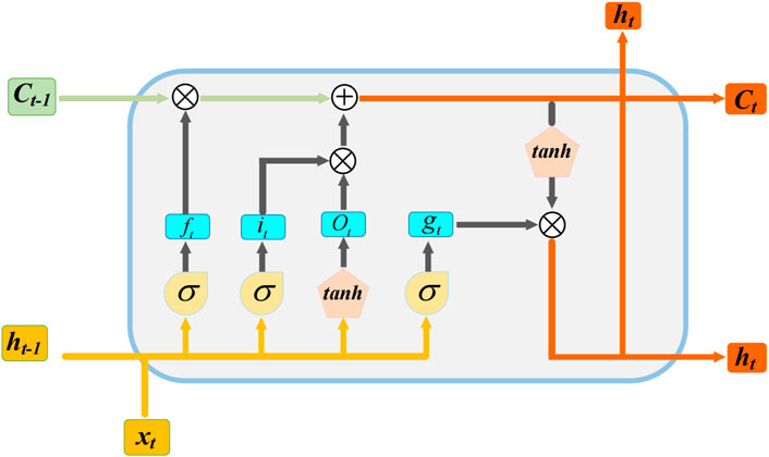
FIGURE 1. The classical LSTM module.

where, h_t−1 denotes the output of the previous cell, x_t denotes the input of the current cell, and σ denotes the sigmoid activation function.

Next, the LSTM determines which information is stored in the cell state through the input gate sigmoid layer for selective memory. A new vector ${\tilde{C}}_t$ is created by the tanh layer to receive the hidden states and current inputs. The tanh layer and the sigmoid layer are then combined to update the state of the cell Liu et al. (2022a); Gruber and Jockisch (2020).

After that, the LSTM updates the old cell state C_t−1 to C_t to determine how to update the information:

$C_t=f_t{C}_{t-1}+i_t\widetilde{C_t}(9)$

Finally, the LSTM outputs the state features of the cell through the output gate sigmoid layer and passes the cell state through the tanh layer to obtain a vector between −1 and 1. This vector is multiplied with the output weights obtained from the output gate to obtain the final output of the LSTM unit.

$o_t=\sigma \left(W_o\left[h_{t-1},x_t\right]+b_o\right)(10)$

$h_t=o_t*\mathit{tanh}\left(C_t\right)(11)$

Different LSTM modules can be stacked together to form a multi-layer LSTM, and by adding depth to the network, the training efficiency can be improved. Figure 2 briefly shows the connection states of different LSTM modules.

FIGURE 2

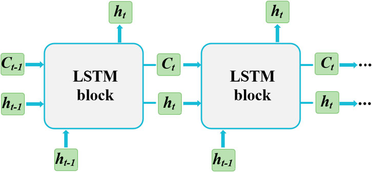
FIGURE 2. Connection of two different LSTM modules.

The proposed deep neural network structure in this paper is shown in Figure 3. It consists of two main parts: the upper part is a CNN, and the lower part is an LSTM. First, the CNN extracts and integrates features from the historical light data of each distributed power plant through convolutional kernels. However, due to filter limitations, the temporal correlation in the input variables cannot be obtained. Second, the LSTM neural network, with the introduction of gating units, can learn the dependent features before and after the input data sequence to obtain the temporal correlation, which makes up for the deficiency of the CNN. Therefore, in this paper, CNN and LSTM are cascaded to form a deep neural network spatiotemporal prediction model. Finally, the LSTM memorizes and filters the integrated features, fits the prediction, and outputs the prediction results through the fully connected layer Ozcanli and Baysal (2022); Dolatabadi et al. (2021); Sinha et al. (2021).

FIGURE 3

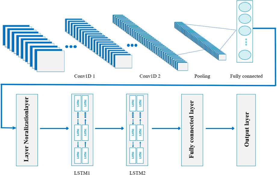
FIGURE 3. The proposed deep learning network structure.

3 Experimental tests

3.1 Experimental data

The data used in this study were obtained from the Oahu Island PV plant data provided by the National Renewable Energy Laboratory (NREL). Oahu Island is located at latitude 21.31°N and longitude 158.08°W. There are 17 distributed PV plants on the island, and the data is collected at a frequency of one sample per second, recording the solar radiation from 5:00 a.m. to 8:00 p.m., spanning the period from March 2010 to October 2011. Before training the original data, the dataset was randomly shuffled and divided into three parts: 70% for training, 20% for validation, and 10% for testing.

3.2 Experiment design and evaluation criteria

In this study, the next data point is predicted using the first ten data points, i.e., the model uses the first 10 seconds of data to predict the next data point. The accuracy of the model prediction is evaluated using three error evaluation criteria, namely mean absolute error (MAE), root mean square error (RMSE), and the coefficient of determination (R2). A smaller difference between the predicted and actual values indicates a better model prediction result.

The MAE indicates the average of the absolute error between the predicted and actual values, whereas the RMSE reflects the degree of deviation from the forecast. The R2 statistically assesses the overall goodness of fit of the model, and a value closer to 1 indicates a better fit. The formulae for calculating the three error metrics are as follows:

$RMSE=\sqrt{\frac{1}{N}\sum _{n=1}^N{\left(\widehat{y}\left(n\right)-y\left(n\right)\right)}^2}(12)$

$MAE=\frac{1}{N}\sum _{n=1}^N\left|\widehat{y}\left(n\right)-y\left(n\right)\right|(13)$

$R^2=1-\frac{{\sum }_{n=1}^N{\left(\widehat{y}\left(n\right)-y\left(n\right)\right)}^2}{{\sum }_{n=1}^N{\left(\widehat{y}\left(n\right)-\bar{y}\left(n\right)\right)}^2}(14)$

where, $\widehat{y}(n)$, y(n), and $\bar{y}(n)$ are the predicted, actual, and mean solar radiation values, respectively, and N is the total number of samples.

3.3 Model structure and hyperparameters

The model has a total of 14 layers of network, the CNN part has 9 layers of network, the first layer is the input layer, the second to the seventh layer are two iterations of convolution, activation and regularization layers. Since the convolution is performed on time series data, both convolutional layers are 1-D convolutional layer, The dimensions of the input data and output data are both two-dimensional, The size of the convolution kernel is 3 and moves in one direction only, the number of convolutional kernels is 32, 64, the step size is 2, 3, and the patch is 2. The activation function of both activation layers is ReLU, and both normalization layers are layerNormalizationLayer (LN). The eighth layer is the pooling layer, and the maximum pooling is chosen to prevent overfitting with size x. The ninth layer is the fully connected layer, which is used to connect to the LSTM network. The 10th layer is layerNormalizationLayer, LN acts as a normalization. Both batchNormalizationLayer (BN) and LN can suppress gradient disappearance and gradient explosion relatively well, but LN is more suitable for sequential networks like LSTM. the LSTM part of the network has 4 layers. Since increasing the depth of the network and the number of hidden cells can help improve the prediction accuracy, the 11th and 12th layers are set as LSTM layers with 256 and 512 hidden cells respectively. The 13th layer is a fully connected layer. Finally, the predicted values are output by regressionLayer. The regression layer calculates the semi-mean-square error loss of the regression task. For regression problems, this layer must be located after the final fully connected layer.

To address the issue of slow convergence and low model accuracy, the model parameters were tuned. The training period was initially set to 80 rounds with 295 iterations per round. The Adam optimizer was used instead of the traditional SGD optimizer to prevent gradient saturation, as it combines the characteristics of AdaGrad and RMSProp to balance the gradient direction and learning rate step. The initial learning rate was set to 0.005, and the activation function used was ReLU or Leaky ReLU. After several experiments, the training period was extended to 100 rounds, the learning rate was reduced to 0.003, and the ReLU activation function was selected.

The specific parameter settings of the model proposed in this paper are displayed in Table 1.

TABLE 1

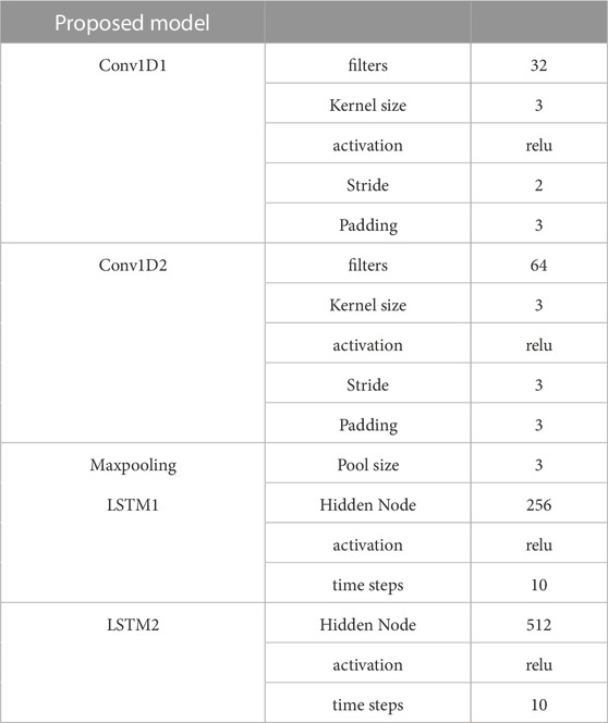
TABLE 1. The specific parameters settings of the proposed model.

3.4 Comparison of the experimental results

Figure 4 illustrates the dynamic loss of the three models during training and validation. The loss decreases as the number of training cycles increases, indicating an improvement in the prediction accuracy of the models. In DNN model training, the number of epochs determines how many times the model works on the entire dataset, and each epoch signifies that the model has undergone a forward and backward propagation. As seen in Figure 4, The training losses of all three models have an overall decreasing trend but fluctuate, which is due to the fact that the direction of gradient descent in each round of the training process of the neural network is not necessarily the overall optimal solution, so the losses do not necessarily decrease compared to the previous round. The proposed model’s loss convergence is faster than the LSTM and CNN models, and the final loss value is smaller than the other models for both the training and validation datasets. This is an intuitive demonstration of the dominance of our proposed model.

FIGURE 4

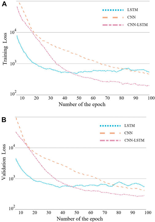
FIGURE 4. (A) Comparison of the training process. (B) Comparison of the validation process.

In order to verify the superior performance of the hybrid model, this study selected the solar radiation data from 5 November 2011, for model training. The prediction results of the 17 distributed PV plants on Oahu Island are shown in Figure 5. The prediction time spanned from 5:00 a.m. to 8:00 p.m. The predicted curve fits well with the actual value curve, indicating that the proposed model has a better prediction effect.

FIGURE 5

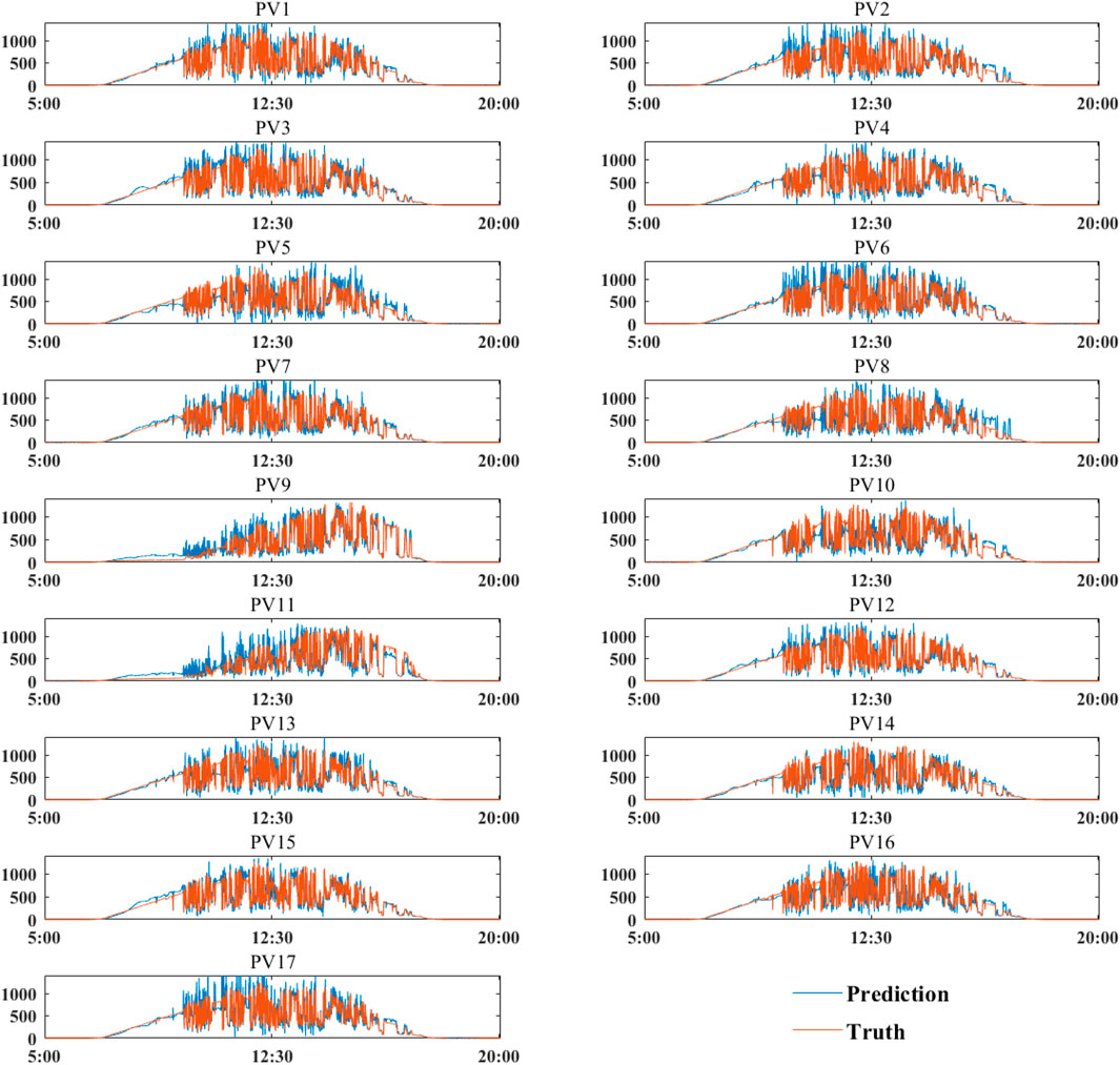
FIGURE 5. Prediction results of solar radiation on Oahu Island on 5 November 2011, using the proposed model.

Figure 6 shows the regression plots for the 17 sites, demonstrating the degree of fit between the data and the regression line. It can be seen that only a few data points deviate slightly from the regression line, and the rest of the data points are evenly distributed on both sides of the regression line, descending along a 45-degree line. The R-value of each site reaches 0.99, further demonstrating the superior prediction effect of the proposed model.

FIGURE 6

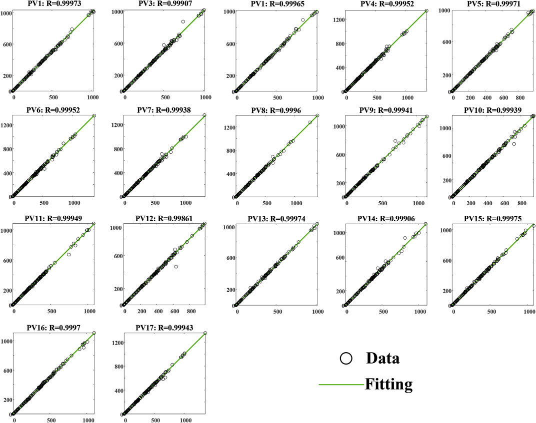
FIGURE 6. Regression plots for 17 sites predicted by the proposed model.

To compare the performance of LSTM, CNN, and the proposed model, they were validated using the same dataset for training. Table 2 shows their respective errors, from which it can be seen that the LSTM model has the largest error, and the proposed model is significantly better than the other two models. The reason behind this is that LSTM lacks temporal learning, and its before-and-after feedback mechanism can only extract some data features, resulting in poorer prediction accuracy. On the other hand, the proposed model adds the CNN structure, which extracts and filters temporal features, discards useless information, enhances useful information, and fully extracts features, thus improving prediction accuracy.

TABLE 2

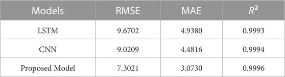
TABLE 2. Performance comparison of Models.

In order to make the comparison more rigorous, we added a set of comparisons by inputting the data of 17 sites into the LSTM for training. From Figure 7 and Figure 8, we can see that the LSTM is significantly worse than our proposed model, thus illustrating that the existence of strong spatial correlation among 17 sites can improve the prediction accuracy. In addition, we also used a single CNN and LSTM model for training on the same dataset, and from the results, our proposed CNN-LSTM model is superior. Figure 9 and Figure 10 shows the comparison between the proposed model and other models evaluation indexes.

FIGURE 7

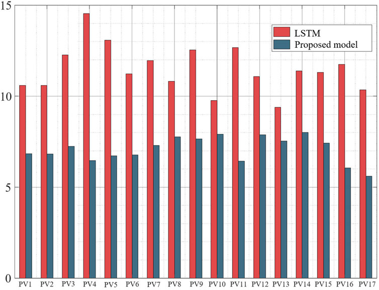
FIGURE 7. RMSE comparison.

FIGURE 8

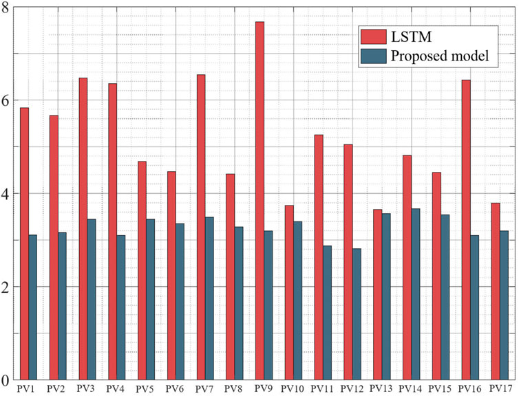
FIGURE 8. MAE comparison.

FIGURE 9

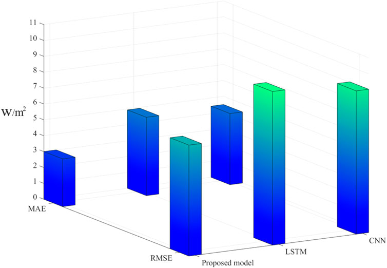
FIGURE 9. Error histograms comparison among the models.

FIGURE 10

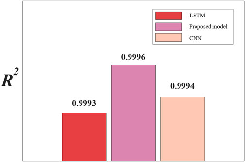
FIGURE 10. R² value histogram comparison among the models.

4 Conclusion

In this paper, a spatio-temporal prediction scheme based on a deep learning model is proposed to capture the strongly correlated spatial relationships among distributed PV generation systems. The proposed model leverages long and short-term memory networks and convolutional neural network models to extract spatio-temporal features from historical data and integrate them using neural networks. Compared with single CNN and LSTM models, the proposed model achieves significant improvements in RMSE and MAE of 19% and 31%, and 24% and 38%, respectively, demonstrating its effectiveness in improving prediction accuracy for practical engineering applications. Future work may explore other combined models and compare their performance with the proposed deep learning model.

Data availability statement

Publicly available datasets were analyzed in this study. This data can be found here: https://midcdmz.nrel.gov/apps/rawdata.pl?site=oahugrid;data=Oahu_GHI;type=zipdata.

Author contributions

QD conceived and completed this paper. XH and RY supported the writing and the review of this paper. YH and RY supported the software utilization. XH, YH, and RY supported the program coding. QD supported the building modelling. All authors contributed to the article and approved the submitted version.

Funding

This research was funded by science and technology project of State Grid Jiangsu Electric Power Co., Ltd. (Research on The research of distribution network distributed photovoltaic high-precision prediction and local consumption capacity, Grant No. J2022043).

Conflict of interest

QD, XH, and YH were employed by the Company State Grid Jiangsu Electric Power Co., Ltd. and RY was employed by the State Grid Xuzhou Power Supply Company of Jiangsu Electric Power Co.

The authors declare that this study received funding from State Grid Jiangsu Electric Power Co., Ltd. The funder had the following involvement in the study: Research on the research of distribution network distributed photovoltaic high-precision prediction and local consumption capacity.

Publisher’s note

All claims expressed in this article are solely those of the authors and do not necessarily represent those of their affiliated organizations, or those of the publisher, the editors and the reviewers. Any product that may be evaluated in this article, or claim that may be made by its manufacturer, is not guaranteed or endorsed by the publisher.

References

Agga, A., Abbou, A., Labbadi, M., El Houm, Y., and Ali, I. H. O. (2022). Cnn-lstm: An efficient hybrid deep learning architecture for predicting short-term photovoltaic power production. Electr. Power Syst. Res.208, 107908. doi:10.1016/j.epsr.2022.107908

CrossRef Full Text | Google Scholar

Agga, A., Abbou, A., Labbadi, M., and El Houm, Y. (2021). Short-term self consumption pv plant power production forecasts based on hybrid cnn-lstm, convlstm models. Renew. Energy177, 101–112. doi:10.1016/j.renene.2021.05.095

CrossRef Full Text | Google Scholar

Bandarra Filho, E. P., Amjad, M., Martins, G., and Mendoza, O. H. (2023). Analysis of the generation potential of hybrid solar power plants. Front. Energy Res.11, 186. doi:10.3389/fenrg.2023.1017943

CrossRef Full Text | Google Scholar

Dolatabadi, A., Abdeltawab, H., and Mohamed, Y. A.-R. I. (2021). Deep spatial-temporal 2-d cnn-blstm model for ultrashort-term lidar-assisted wind turbine’s power and fatigue load forecasting. IEEE Trans. Industrial Inf.18, 2342–2353. doi:10.1109/tii.2021.3097716

CrossRef Full Text | Google Scholar

Gruber, N., and Jockisch, A. (2020). Are gru cells more specific and lstm cells more sensitive in motive classification of text?Front. Artif. Intell.3, 40. doi:10.3389/frai.2020.00040

PubMed Abstract | CrossRef Full Text | Google Scholar

Gupta, A. K., and Singh, R. K. (2022). Short-term day-ahead photovoltaic output forecasting using pca-sfla-grnn algorithm. Front. Energy Res.10, 1029449. doi:10.3389/fenrg.2022.1029449

CrossRef Full Text | Google Scholar

Haputhanthri, D., De Silva, D., Sierla, S., Alahakoon, D., Nawaratne, R., Jennings, A., et al. (2021). Solar irradiance nowcasting for virtual power plants using multimodal long short-term memory networks. Front. Energy Res.9, 722212. doi:10.3389/fenrg.2021.722212

CrossRef Full Text | Google Scholar

Jiao, X., Li, X., Lin, D., and Xiao, W. (2021). A graph neural network based deep learning predictor for spatio-temporal group solar irradiance forecasting. IEEE Trans. Industrial Inf.18, 6142–6149. doi:10.1109/tii.2021.3133289

CrossRef Full Text | Google Scholar

Jurado, M., Samper, M., and Rosés, R. (2023). An improved encoder-decoder-based cnn model for probabilistic short-term load and pv forecasting. Electr. Power Syst. Res.217, 109153. doi:10.1016/j.epsr.2023.109153

CrossRef Full Text | Google Scholar

Karalus, S., Köpfer, B., Guthke, P., Killinger, S., and Lorenz, E. (2023). Analysing grid-level effects of photovoltaic self-consumption using a stochastic bottom-up model of prosumer systems. Energies16, 3059. doi:10.3390/en16073059

CrossRef Full Text | Google Scholar

Khan, P. W., Byun, Y.-C., and Lee, S.-J. (2022). Optimal photovoltaic panel direction and tilt angle prediction using stacking ensemble learning. Front. Energy Res.10, 382. doi:10.3389/fenrg.2022.865413

CrossRef Full Text | Google Scholar

Kim, T.-Y., and Cho, S.-B. (2019). Predicting residential energy consumption using cnn-lstm neural networks. Energy182, 72–81. doi:10.1016/j.energy.2019.05.230

CrossRef Full Text | Google Scholar

Kollipara, Keerthi, D., and Ravi Sankar, R. (2022). Energy efficient photovoltaic-electric spring for real and reactive power control in demand side management. Front. Energy Res.974. doi:10.3389/fenrg.2022.762931

CrossRef Full Text | Google Scholar

Li, Z., Xu, R., Luo, X., Cao, X., Du, S., and Sun, H. (2022). Short-term photovoltaic power prediction based on modal reconstruction and hybrid deep learning model. Energy Rep.8, 9919–9932. doi:10.1016/j.egyr.2022.07.176

CrossRef Full Text | Google Scholar

Liao, M., Zhang, Z., Jia, J., Xiong, J., and Han, M. (2022). Mapping China’s photovoltaic power geographies: Spatial-temporal evolution, provincial competition and low-carbon transition. Renew. Energy191, 251–260. doi:10.1016/j.renene.2022.03.068

CrossRef Full Text | Google Scholar

Liu, R., Wei, J., Sun, G., Muyeen, S., Lin, S., and Li, F. (2022a). A short-term probabilistic photovoltaic power prediction method based on feature selection and improved lstm neural network. Electr. Power Syst. Res.210, 108069. doi:10.1016/j.epsr.2022.108069

CrossRef Full Text | Google Scholar

Liu, X., Guo, W., Feng, Q., and Wang, P. (2022b). Spatial correlation, driving factors and dynamic spatial spillover of electricity consumption in China: A perspective on industry heterogeneity. Energy257, 124756. doi:10.1016/j.energy.2022.124756

CrossRef Full Text | Google Scholar

Ortiz, M. M., Kvalbein, L., and Hellemo, L. (2021). Evaluation of open photovoltaic and wind production time series for Norwegian locations. Energy236, 121409. doi:10.1016/j.energy.2021.121409

CrossRef Full Text | Google Scholar

Ozcanli, A. K., and Baysal, M. (2022). Islanding detection in microgrid using deep learning based on 1d cnn and cnn-lstm networks. Sustain. Energy, Grids Netw.32, 100839. doi:10.1016/j.segan.2022.100839

CrossRef Full Text | Google Scholar

Sim, H., and Lee, J. (2020). Bitstream-based neural network for scalable, efficient, and accurate deep learning hardware. Front. Neurosci.14, 543472. doi:10.3389/fnins.2020.543472

PubMed Abstract | CrossRef Full Text | Google Scholar

Sinha, A., Tayal, R., Vyas, A., Pandey, P., and Vyas, O. (2021). Forecasting electricity load with hybrid scalable model based on stacked non linear residual approach. Front. Energy Res.9, 682. doi:10.3389/fenrg.2021.720406

CrossRef Full Text | Google Scholar

Song, H., Al Khafaf, N., Kamoona, A., Sajjadi, S. S., Amani, A. M., Jalili, M., et al. (2023). Multitasking recurrent neural network for photovoltaic power generation prediction. Energy Rep.9, 369–376. doi:10.1016/j.egyr.2023.01.008

CrossRef Full Text | Google Scholar

Stüber, M., Scherhag, F., Deru, M., Ndiaye, A., Sakha, M. M., Brandherm, B., et al. (2021). Forecast quality of physics-based and data-driven pv performance models for a small-scale pv system. Front. Energy Res.9, 639346. doi:10.3389/fenrg.2021.639346

CrossRef Full Text | Google Scholar

Voyant, C., Notton, G., Kalogirou, S., Nivet, M.-L., Paoli, C., Motte, F., et al. (2017). Machine learning methods for solar radiation forecasting: A review. Renew. energy105, 569–582. doi:10.1016/j.renene.2016.12.095

CrossRef Full Text | Google Scholar