Stability analysis of two-terminal HVDC transmission systems using SISO open-loop gains

The ports of a three-phase voltage source converter have multiple frequency electrical parameters, which makes HVDC systems with these converters present multiple input multiple output (MIMO) characteristics. The generalized Nyquist criterion of the MIMO model is often used to analyze the system stability. However, this model is more difficult to obtain than the single-input single-output (SISO) model, and the stability margin and the oscillation frequency band are difficult to capture. To solve these problems, this paper took the two-terminal HVDC transmission system as the research object to derive a SISO model that can be measured by a port. Moreover, this study also proposed a method for analyzing the system stability through envelope SISO open-loop gains. Finally, the key port and parameters affecting the system stability were analyzed according to the stability margin, which provided theoretical support for the design of the system parameters. The established model and the proposed analysis method were verified in a MATLAB/Simulink simulation model.

1 Introduction

With the increase in transmission capacity, HVDC systems have become an ideal transmission solution (Flourentzou et al., 2009). However, this has brought about concerns related to the stability of the interconnected systems (Sun et al., 2017). The small-signal stability of HVDC systems can be studied using state space model-based eigenvalue analysis (Du et al., 2018; Dewangan and Bahirat, 2020) and impedance models (Chang et al., 2021)- (Cao et al., 2017). However, as the establishment of a state space model requires detailed parameters, this model cannot be used when model parameters are unknown or user privacy is protected. Because the impedance model can be obtained by port measurement, stability analysis based on the impedance model has been widely studied and applied in recent years.

System stability is analyzed based on DC single-input single-output (SISO) impedance models (Chang et al., 2021) or AC SISO impedance models of two-terminal DC transmission systems (Sun, 2011). To facilitate the analysis of the system stability, the sending end converter of the system is equivalent to a constant voltage source (Shah and Parsa, 2017) or constant power (Zou et al., 2018), and the simplified model is used to analyze the system stability. Bo et al. (2017) established the second-order impedance matrix of the converter in the rotating coordinate system and demonstrated that when the converter operates at a specific high-power factor, the coupling of the dq axis can be ignored and the MIMO model is reduced to the SISO model. Chou et al. (2020) also analyzed the system stability based on two SISO port models. However, multiple frequency interactions occur between the AC and DC ports of voltage source converters. If a single-frequency small signal voltage disturbance appears on the AC side of the converter, dual-frequency AC currents can be generated. These dual-frequency currents generate the disturbance voltage response of the corresponding frequency so that the two frequencies on the AC side are coupled to each other. At the same time, another frequency of current response also is produced at the DC port (Zhang et al., 2019a). Multi-frequency AC-DC interactions exist in two-terminal HVDC transmission systems (Tan et al., 2020). The AC-DC interactions are ignored in these models, which may cause errors in stability determination (Huang and Wang, 2018).

Zou et al. (2018) analyzed system stability according to the positive and negative sequence SISO impedances of a single partition point. Sun 2021) used the DC port impedance ratio considering the interactions to determine the system stability based on the Nyquist criterion. These systems must determine the number of zeros and poles in the right half-plane of the subsystems. Zhang et al. (2020) and Fan and Miao (2020) pointed out that system models of a single partition point may not accurately determine the global stability of the system but did not report on partition point selection. Cao et al. (2017) and Eto et al. (2023) used iterative analyses to ensure that there were no zeros in the right half-plane of the subsystem impedance at a single partition point, and then determined the system stability. Liu et al. (2014) determined the system stability by the system equivalent impedance sum. However, in practical applications, it is difficult to determine the number of zeros and poles in the right half-plane; moreover, it is also difficult to obtain the stability margin. Sun (2022) and Zhang et al. (2019b) determined the system stability by analyzing the SISO transfer function of multiple control loops in a single grid-connected inverter. However, this method was not used in the two-terminal HVDC transmission system. Zhu et al. (2023) used the 6-order MIMO admittance parameter matrix to describe the AC-DC port interactions of the system and analyzed the system stability using the generalized Nyquist eigenvalue. Zhang et al. (2021) used the determinant phases between the system MIMO admittance matrix and the grid impedance in the full frequency band to judge the system stability. However, in analysis methods based on the MIMO system model, it is difficult to capture the oscillation frequency band of the system and obtain the stability margin. The stability margin is a key indicator of the system’s robustness. A stability margin is necessary for parameter design in practical engineering (Healey, 1976; Yang et al., 2021).

To accurately analyze the system stability and obtain the stability margin of the system, this paper used the two-terminal HVDC transmission system as the research object and determined the ports for analyzing the system stability by introducing the envelope division system. Based on the port parameter matrix representing the AC-DC interactions of the system sub-module, the SISO open-loop gains of the system were obtained. Based on the SISO open-loop gains of the ports, the oscillation frequency band of the system was analyzed to avoid screening of the zero and pole points in the right half-plane. Finally, the key modules and parameters affecting the system stability were identified. The research results provide a theoretical basis for accurate parameter design.

The rest of this report is arranged as follows. Section 2 establishes the port parameter matrix model of each module of the system. Section 3 takes the two-terminal HVDC system as the research object. Based on the envelope division system, the SISO port equivalent impedance/admittance model of the system is derived and the accuracy of the model is verified. Section 4 analyzes the system stability based on the SISO model established by the envelope. The key parameters affecting the system stability are identified in Section 5. Section 6 summarizes this work.

2 Port models of the system submodules

The two-terminal HVDC transmission system consists of two converters and a DC network. The port parameter matrixes of the HVDC system sub-modules and AC grids are established in this section.

The main circuit diagram of the two-terminal HVDC transmission system is shown in Figure 1. The VSC1 is a rectifier with current control. The VSC2 controls the DC voltage. $v_{pa}$, $v_{pb}$, $v_{pc}$, $i_{pa}$, $i_{pb}$, and $i_{pc}$ are the three-phase AC voltage and the AC current of the converter, respectively. $H_i\left(s\right)$ is the current control loop. $H_i\left(s\right)=K_{pi}+K_{ii}/s$, $K_{pi}$ and $K_{ii}$ are the proportional and integral coefficients of the current PI control, respectively. ${\theta }_{pll}$ is the output phase angle of the PLL. $H_{pll}\left(s\right)$ is an open-loop small-signal model of the phase-locked loop (PLL). $I_{dref}$ and $I_{qref}$ are the dq axis reference current of the converter. L is the converter AC filter inductance. $v_{dcj}$ and $i_{dcj}$ are DC voltage and current, respectively. $Z_{line}$ and $Z_f$ are the equivalent impedances of transmission lines and DC filters, respectively.

FIGURE 1

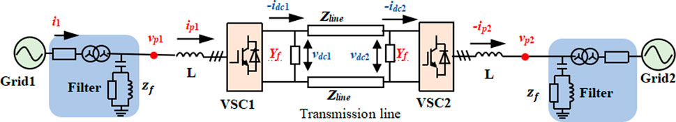
FIGURE 1. Structure of the HVDC transmission system.

2.1 Admittance parameter models of the converter modules

Based on the AC-DC interactions at the ports of the three-phase converter, the admittance parameter matrix of the three-phase converter in the stationary coordinate system can be expressed as

$\left[\begin{array}{c}{I}_{dcj}\left(s-j{\omega }_1\right)\\ \begin{array}{c}{I}_{pj}\left(s\right)\\ I_{pj}\left(s-j2{\omega }_1\right)\end{array}\end{array}\right]=\left[\begin{array}{ccc}{Y}_{ssj}\left(s\right)& Y_{spj}\left(s\right)& Y_{snj}\left(s\right)\\ Y_{psj}\left(s\right)& Y_{ppj}\left(s\right)& Y_{pnj}\left(s\right)\\ Y_{nsj}\left(s\right)& Y_{npj}\left(s\right)& Y_{nnj}\left(s\right)\end{array}\right]\left[\begin{array}{c}{V}_{dcj}\left(s-j{\omega }_1\right)\\ \begin{array}{c}{V}_{pj}\left(s\right)\\ V_{pj}\left(s-j2{\omega }_1\right)\end{array}\end{array}\right],(1)$

where ${\omega }_1=2\pi f_1$, $f_1$ is the fundamental frequency; $I_{pj}\left(s\right)$, $I_{pj}\left(s-j2{\omega }_1\right)$, $V_{pj}\left(s\right),$ and $V_{pj}\left(s-j2{\omega }_1\right)$ are the three-phase AC current and voltage small signal models at different frequencies of the jth converter; and $I_{dcj}\left(s-j{\omega }_1\right)$ and $V_{dcj}\left(s-j{\omega }_1\right)$ are the DC current and voltage of the jth converter, respectively.

The parameters in the matrix model represent the interactions between the voltage disturbances of the converter at different frequencies and the corresponding current responses. The main diagonal element is the admittance of the converter port voltage interference and the current response at the same frequency. The remaining admittance elements characterize the relationship between the converter port voltage disturebances and the current responses at different frequencies. Each admittance parameter is derived when the other voltage disturbances except the corresponding voltage disturbances are short-circuited. The specific derivation is as follows.

A perturbation $V_{pj}\left(s\right)$ on the AC side of the system inverter results in a small perturbation at the output phase by the PLL. Based on the structure of the PLL in Zou et al. (2018), the relationship between the variables in the stationary reference frame and the rotating coordinate system can be obtained as

$X_{dqj}\left(s-j{\omega }_1\right)=X_{p\mathrm{j}}\left(s\right)-0.5X_{dqj}{T}_{pll}\left(s-j{\omega }_1\right)V_{pj}\left(s\right),(2)$

$X_{dqj}\left({j\omega }_1-s\right)=X_{pj}\left({2j\omega }_1-s\right)+0.5X_{dqj}{T}_{pll}\left(j{\omega }_1-s\right)V_{pj}^{*}\left(s\right),(3)$

where X represents the AC current, voltage, or duty cycle D of the converter; $X_{dqj}$ and $X_{dqj}\left(s-j{\omega }_1\right)$ are the steady-state complex coefficient and small signal model, respectively; $X_{dqj}=X_{dj}+X_{qj}$. $X_{p\mathrm{j}}\left(s\right)$ is a small-signal model of AC current, voltage, or duty cycle in the stationary coordinate system; $V_{pj}^{*}\left(s\right)$ is the conjugate quantity of $V_{pj}\left(s\right)$; and $T_{pll}\left(s-j{\omega }_1\right)$ is the closed loop transfer function of the PLL, $T_{pll}\left(s\right)=H_{pll}\left(s\right)/\left[1+V_1{H}_{pll}\left(s\right)\right]$.

The small signal model of the main circuit and the current loop in the Appendix can be derived as

$sL{I}_{pj}\left(s\right)=D_{pj}\left(s\right)V_{dcj}-V_{pj}\left(s\right),(4)$

$\left(2j{\omega }_1-s\right)L{I}_{pj}\left(2j{\omega }_1-s\right)=D_{pj}\left(j2{\omega }_1-s\right)V_{dcj},(5)$

${\mathrm{D}}_{dqj}\left(s\right)=\frac{1}{2V_{cr}}\left[-H_i\left(s\right)+j{\omega }_{1}L\right]I_{dqj}\left(\mathrm{s}\right),(6)$

where L is the converter AC filter inductor.

According to the small signal relationship between the main circuit and the control circuit (6), the relationship between the voltage disturbance $V_{pj}\left(s\right)$ and the current response can be derived as

$Y_{ppj}\left(s\right)=\frac{I_{pj}\left(s\right)}{V_{pj}\left(s\right)}=\frac{1-0.5V_{dcj}{\mathrm{D}}_{dqj}{\mathrm{T}}_{pll}\left(s-j{\omega }_1\right)+\left[{j\omega }_{1}L-H_i\left(s-j{\omega }_1\right)\right]0.5{\mathrm{I}}_{dqj}{\mathrm{T}}_{PLL}\left(s-j{\omega }_1\right)}{\left(s-j{\omega }_1\right)L+H_i\left(s-j{\omega }_1\right)},(7)$

where $H_i\left(s\right)$ is the current control loop; $T_{pll}\left(s-j{\omega }_1\right)$ is the closed loop transfer function of the PLL, $T_{pll}\left(s\right)=H_{pll}\left(s\right)/\left[1+V_1{H}_{pll}\left(s\right)\right]$; $H_{pll}\left(s\right)$ is an open-loop small-signal model of the PLL; $V_{dcj}$ is the steady-state DC voltage of the jth converter; and ${\mathrm{I}}_{dqj}$ and ${\mathrm{D}}_{dqj}$ are the steady-state values of AC current and duty cycle, respectively.

Similarly, the relationship between the small disturbance and response of the converter at different frequencies in the main circuit and the control circuit can be deduced. The specific formula is shown in the Appendix.

2.2 Parameter models for AC and DC networks

The DC network of the system is composed of DC transmission lines and DC filters. The transmission parameter matrix of the DC network port is described as

$\left[\begin{array}{c}{V}_{dc2}\left(s-j{\omega }_1\right)\\ I_{dc2}\left(s-j{\omega }_1\right)\end{array}\right]={\mathit{T}}_{\mathit{d}\mathit{c}\mathit{n}}\left(s\right)\left[\begin{array}{c}{V}_{dc1}\left(s-j{\omega }_1\right)\\ I_{dc1}\left(s-j{\omega }_1\right)\end{array}\right],(8)$

where ${\mathit{T}}_{\mathit{d}\mathit{c}\mathit{n}}\left(s\right)={\mathit{T}}_{\mathit{c}\mathbf{1}}\left(s\right)*{\mathit{T}}_{\mathit{d}\mathit{c}\mathit{l}}\left(s\right)*{\mathit{T}}_{\mathit{c}\mathbf{2}}\left(s\right)$; ${\mathit{T}}_{\mathit{c}\mathbf{1}}\left(s\right)$ and ${\mathit{T}}_{\mathit{c}\mathbf{2}}\left(s\right)$ are the transmission parameter matrix of the rectifier and inverter DC filter; and ${\mathit{T}}_{\mathit{d}\mathit{c}\mathit{l}}\left(s\right)$ is the transmission parameter matrix of the DC transmission line.

${\mathit{T}}_{\mathit{c}\mathit{j}}\left(s\right)=\left[\begin{array}{cc}1& 0\\ -Y_f\left(s-j{\omega }_1\right)& 1\end{array}\right],(9)$

${\mathit{T}}_{\mathit{d}\mathit{c}\mathit{l}}\left(s\right)=\left[\begin{array}{cc}1& -2Z_{line}\left(s-j{\omega }_1\right)\\ 0& 1\end{array}\right],(10)$

where $Y_f\left(s-j{\omega }_1\right)$ and $Z_{line}\left(s-j{\omega }_1\right)$ are the equivalent admittance of the DC filter and the equivalent impedance of the DC transmission line, respectively.

The impedance parameter matrix ${\mathit{Z}}_{\mathit{d}\mathit{c}\mathit{n}}\left(s\right)$ of the DC network can be obtained by the transmission parameter matrix conversion.

$\left[\begin{array}{c}{V}_{dc1}\left(s-j{\omega }_1\right)\\ V_{dc2}\left(s-j{\omega }_1\right)\end{array}\right]={\mathit{Z}}_{\mathit{d}\mathit{c}\mathit{n}}\left(s\right)\left[\begin{array}{c}{I}_{dc1}\left(s-j{\omega }_1\right)\\ I_{dc2}\left(s-j{\omega }_1\right)\end{array}\right]=\left[\begin{array}{cc}{Z}_{n11}\left(s\right)& Z_{n12}\left(s\right)\\ Z_{n21}\left(s\right)& Z_{n22}\left(s\right)\end{array}\right]\left[\begin{array}{c}{I}_{dc1}\left(s-j{\omega }_1\right)\\ I_{dc2}\left(s-j{\omega }_1\right)\end{array}\right].(11)$

The elements in the matrix are the impedance parameters of the DC network. $Z_{n11}\left(s\right)$ and $Z_{n22}\left(s\right)$ are the input impedances of DC ports B and D, respectively, and $Z_{n12}\left(s\right)$ and $Z_{n21}\left(s\right)$ are the transfer impedances between DC ports B and D, respectively.

The port impedance parameter model ${\mathit{Z}}_{\mathit{g}\mathit{z}}\left(\mathit{s}\right)$ of the AC grids is expressed as

$\left[\begin{array}{c}\begin{array}{c}{V}_{p1}\left(s\right)\\ V_{p1}\left(s-j2{\omega }_1\right)\\ V_{p2}\left(s\right)\end{array}\\ V_{p2}\left(s-j2{\omega }_1\right)\end{array}\right]={\mathit{Z}}_{\mathit{g}\mathit{z}}\left(\mathit{s}\right)\left[\begin{array}{c}\begin{array}{c}{I}_{p1}\left(s\right)\\ I_{p1}\left(s-j2{\omega }_1\right)\\ -I_{p2}\left(s\right)\end{array}\\ {-I}_{p2}\left(s-j2{\omega }_1\right)\end{array}\right]=\left[\begin{array}{cc}{\mathit{Z}}_{\mathit{g}\mathbf{1}}& \mathbf{0}\\ \mathbf{0}& {\mathit{Z}}_{\mathit{g}\mathbf{2}}\end{array}\right]\left[\begin{array}{c}\begin{array}{c}{I}_{p1}\left(s\right)\\ I_{p1}\left(s-j2{\omega }_1\right)\\ -I_{p2}\left(s\right)\end{array}\\ {-I}_{p2}\left(s-j2{\omega }_1\right)\end{array}\right],(12)$

where ${\mathit{Z}}_{\mathit{g}\mathit{j}}$ is the equivalent impedance model of the AC grid j.

${\mathit{Z}}_{\mathit{g}\mathit{j}}=\left[\begin{array}{cc}{Z}_{gj}\left(s\right)& 0\\ 0& Z_{gj}\left(s-j2{\omega }_1\right)\end{array}\right].(13)$

3 Stability analysis of HVDC transmission systems

We propose a method for the stability analysis of the HVDC transmission system based on an envelope line and port SISO models. The stability analysis based on the SISO open loop gains can be used to obtain the oscillation frequency band and the stability margin, which provide a theoretical basis for the subsequent parameter design.

3.1 Loop gains of HVDC transmission systems

Different from the system divided by a single partition point, this work proposes to use the envelope line to divide the interconnected system. A closed envelope is formed by cutting the ports of the interconnected system. The purpose of dividing the envelope system is to ensure the stability of the divided subsystem. If the stability of the HVDC transmission system cannot be guaranteed when operating alone, the envelope divides the system into converter and grid subsystems by cutting the AC and DC ports of the system. The converter subsystem consists of two converters, which are designed to operate stably, while the grid subsystem is composed of an AC power grid and a DC transmission network. All components of the grid subsystem are passive, so the subsystem can operate stably. When the envelope is divided into two ends of the HVDC transmission system, as shown in Figure 2, it intersects with the four ports of the system; namely which are AC (ports A and C), and DC (ports B and D), respectively. The system stability of the interconnection between the HVDC transmission system and the weak grid is analyzed based on the impedance ratios of the intersection ports of the envelope line.

FIGURE 2

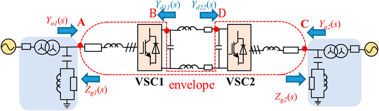
FIGURE 2. Equivalent SISO models and an envelope of the HVDC transmission system.

Therefore, the port models of the system rectifier and inverter can be obtained based on (1). The port admittance parameter model of the HVDC system’s converter module is obtained by port expansion.

$\left[\begin{array}{c}\begin{array}{c}{I}_{dc1}\left(s-j{\omega }_1\right)\\ I_{dc2}\left(s-j{\omega }_1\right)\end{array}\\ \begin{array}{c}{I}_{p1}\left(s\right)\\ I_{p1}\left(s-j2{\omega }_1\right)\\ \begin{array}{c}{I}_{p2}\left(s\right)\\ I_{p2}\left(s-j2{\omega }_1\right)\end{array}\end{array}\end{array}\right]=\left[\begin{array}{cc}{\mathit{Y}}_{\mathit{d}\mathit{d}}\left(\mathit{s}\right)& {\mathit{Y}}_{\mathit{d}\mathit{a}}\left(\mathit{s}\right)\\ {\mathit{Y}}_{\mathit{a}\mathit{d}}\left(\mathit{s}\right)& {\mathit{Y}}_{\mathit{a}\mathit{a}}\left(\mathit{s}\right)\end{array}\right]\left[\begin{array}{c}\begin{array}{c}{V}_{dc1}\left(s-j{\omega }_1\right)\\ V_{dc2}\left(s-j{\omega }_1\right)\end{array}\\ \begin{array}{c}{V}_{p1}\left(s\right)\\ V_{p1}\left(s-j2{\omega }_1\right)\\ \begin{array}{c}{V}_{p2}\left(s\right)\\ V_{p2}\left(s-j2{\omega }_1\right)\end{array}\end{array}\end{array}\right],(14)$

where ${\mathit{Y}}_{\mathit{d}\mathit{d}}\left(\mathit{s}\right)$ and ${\mathit{Y}}_{\mathit{a}\mathit{a}}\left(\mathit{s}\right)$ represent the characteristics of the DC and AC ports of the converters and ${\mathit{Y}}_{\mathit{d}\mathit{a}}\left(\mathit{s}\right)$ and ${\mathit{Y}}_{\mathit{a}\mathit{d}}\left(\mathit{s}\right)$ represent the interactions between the AC and DC ports of the converters, respectively. Because the converter module is stable, the admittance parameter matrix in (14)has no right half-plane pole (RHP).

3.1.1 SISO open-loop gains of AC ports

To obtain the SISO open-loop gains of AC ports A and C, the DC ports of the converter are interconnected with the DC transmission network, and the DC ports are eliminated. The admittance parameter models of two converter AC ports A and C are expressed as

$\left[\begin{array}{c}\begin{array}{c}{I}_{p1}\left(s\right)\\ I_{p1}\left(s-j2{\omega }_1\right)\\ -I_{p2}\left(s\right)\end{array}\\ {-I}_{p2}\left(s-j2{\omega }_1\right)\end{array}\right]=\left[\begin{array}{cc}{\mathit{Y}}_{\mathit{R}\mathit{R}}& {\mathit{Y}\mathit{M}}_{\mathit{R}\mathit{I}}\\ {\mathit{Y}\mathit{M}}_{\mathit{I}\mathit{R}}& {\mathit{Y}}_{\mathit{I}\mathit{I}}\end{array}\right]\left[\begin{array}{c}\begin{array}{c}{V}_{p1}\left(s\right)\\ V_{p1}\left(s-j2{\omega }_1\right)\\ V_{p2}\left(s\right)\end{array}\\ V_{p2}\left(s-j2{\omega }_1\right)\end{array}\right],(15)$

$\left[\begin{array}{cc}{\mathit{Y}}_{\mathit{R}\mathit{R}}& {\mathit{Y}\mathit{M}}_{\mathit{R}\mathit{I}}\\ {\mathit{Y}\mathit{M}}_{\mathit{I}\mathit{R}}& {\mathit{Y}}_{\mathit{I}\mathit{I}}\end{array}\right]={\mathit{Y}}_{\mathit{a}\mathit{a}}\left(s\right)-{\mathit{Y}}_{\mathit{a}\mathit{d}}\left(s\right){\left[{\mathit{Y}}_{\mathit{d}\mathit{c}\mathit{n}}\left(s\right)-{\mathit{Y}}_{\mathit{d}\mathit{d}}\left(s\right)\right]}^{-1}{\mathit{Y}}_{\mathit{d}\mathit{a}}\left(s\right),(16)$

where ${\mathit{Y}}_{\mathit{R}\mathit{R}}$, ${\mathit{Y}}_{\mathit{R}\mathit{I}}$, ${\mathit{Y}\mathit{M}}_{\mathit{I}\mathit{R}}$, and ${\mathit{Y}\mathit{M}}_{\mathit{I}\mathit{I}}$ are 2-order square matrices and ${\mathit{Y}}_{\mathit{R}\mathit{R}}$ and ${\mathit{Y}}_{\mathit{I}\mathit{I}}$ represent the characteristics of the AC port of a single rectifier and a single inverter, respectively. ${\mathit{Y}\mathit{M}}_{\mathit{R}\mathit{I}}$ and ${\mathit{Y}\mathit{M}}_{\mathit{I}\mathit{R}}$ represent the interactions of AC port voltage disturbance and current response between two converters in a two-terminal HVDC system, respectively. Because the converter module of the system is stable, there is no RHP in ${\mathit{Y}}_{\mathit{R}\mathit{R}}$, ${\mathit{Y}}_{\mathit{R}\mathit{I}}$, ${\mathit{Y}\mathit{M}}_{\mathit{I}\mathit{R}}$, and ${\mathit{Y}\mathit{M}}_{\mathit{I}\mathit{I}}$.

The DC port of the HVDC system forms a feedback loop with the DC network. The stability of the feedback loop can be analyzed by the loop transfer function ${\left[{\mathit{Y}}_{\mathit{d}\mathit{c}\mathit{n}}\left(\mathit{s}\right)-{\mathit{Y}}_{\mathit{d}\mathit{d}}\left(\mathit{s}\right)\right]}^{-\mathbf{1}}$. If the feedback loop is unstable, the admittance in (Eq. 16) has right half-plane poles.

When the AC port of the system is connected to the AC grid, the AC port is eliminated to form a feedback loop. The system can be reduced to obtain a second-order matrix of a single AC port. Therefore, the admittance models of port A and port C can be expressed as

$\left[\begin{array}{c}{I}_{p1}\left(s\right)\\ I_{p1}\left(s-j2{\omega }_1\right)\end{array}\right]=\left({\mathit{Y}}_{\mathit{R}\mathit{R}}+{\mathit{Y}}_{\mathit{R}\mathit{I}}{{\mathit{Z}}_{\mathit{g}\mathbf{2}}\left(\mathit{I}-{\mathit{Z}}_{\mathit{g}\mathbf{2}}{\mathit{Y}}_{\mathit{I}\mathit{I}}\right)}^{-1}{\mathit{Y}}_{\mathit{I}\mathit{R}}\right)\left[\begin{array}{c}{V}_{p1}\left(s\right)\\ V_{p1}\left(s-j2{\omega }_1\right)\end{array}\right]=\left[\begin{array}{cc}{YR}_{11}\left(s\right)& {YR}_{12}\left(s\right)\\ {YR}_{21}\left(s\right)& {YR}_{22}\left(s\right)\end{array}\right]\left[\begin{array}{c}{V}_{p1}\left(s\right)\\ V_{p1}\left(s-j2{\omega }_1\right)\end{array}\right],(17)$

$\left[\begin{array}{c}{I}_{p2}\left(s\right)\\ I_{p2}\left(s-j2{\omega }_1\right)\end{array}\right]=\left({\mathit{Y}}_{\mathit{I}\mathit{I}}+{\mathit{Y}}_{\mathit{I}\mathit{R}}{\mathit{Z}}_{\mathit{g}\mathbf{1}}{\left(\mathit{I}-{\mathit{Z}}_{\mathit{g}\mathbf{1}}{\mathit{Y}}_{\mathit{R}\mathit{R}}\right)}^{-1}{\mathit{Y}}_{\mathit{R}\mathit{I}}\right)\left[\begin{array}{c}{V}_{p2}\left(s\right)\\ V_{p2}\left(s-j2{\omega }_1\right)\end{array}\right]=\left[\begin{array}{cc}{YI}_{11}\left(s\right)& {YI}_{12}\left(s\right)\\ {YI}_{21}\left(s\right)& {YI}_{22}\left(s\right)\end{array}\right]\left[\begin{array}{c}{V}_{p2}\left(s\right)\\ V_{p2}\left(s-j2{\omega }_1\right)\end{array}\right],(18)$

where ${YR}_{11}\left(s\right)$, ${YR}_{22}\left(s\right)$, ${YI}_{11}\left(s\right)$, and ${YI}_{22}\left(s\right)$ are the self-admittances of ports A and C, respectively. These admittances represent the relationships between the AC port voltage disturbance and the current response at the same frequency. ${YR}_{12}\left(s\right)$ and ${YR}_{21}\left(s\right)$ are the mutual admittances of port A. ${YI}_{12}\left(s\right)$ and ${YI}_{21}\left(s\right)$ are the mutual admittances of port C. The mutual admittances describe the frequency coupling of ports A or C.

The feedback loops are introduced into the reduced-dimensional system port model. The stability of the two admittance models of ports A and C can be determined by ${\mathit{Z}}_{\mathit{g}\mathbf{2}}{\mathit{Y}}_{\mathit{I}\mathit{I}}$ and ${\mathit{Z}}_{\mathit{g}\mathbf{1}}{\mathit{Y}}_{\mathit{R}\mathit{R}}$.

Due to the port-connected grid impedances, the second-order admittance parameter matrix in (Eq. 17) can be further reduced to a SISO impedance. The SISO impedance model of port A is

$Y_{a1}\left(s\right)={YR}_{11}\left(s\right)+Z_{g1}\left(s-j2{\omega }_1\right){YR}_{12}\left(s\right){\left[1-Z_{g1}\left(s-j2{\omega }_1\right){YR}_{22}\left(s\right)\right]}^{-1}{YR}_{21}\left(s\right),(19)$

where ${YR}_{11}\left(s\right)$ and ${YR}_{22}\left(s\right)$ are the relationship between the same frequency voltage disturbance and the current response of port A, and ${YR}_{12}\left(s\right)$ and ${YR}_{21}\left(s\right)$ describe the frequency coupling of port A.

The transfer function ${GL}_A\left(s\right)$ of port A voltage disturbance and output voltage can be expressed as

${GL}_A\left(s\right)=\frac{V_{p1}\left(s\right)}{V_{g1}\left(s\right)}=\frac{1}{1+H_A\left(s\right)}=\frac{1}{1+Z_{g1}\left(s\right)Y_{a1}\left(s\right)}=\frac{1}{{\left[1-{Z_{g1}\left(s-j2{\omega }_1\right)YR}_{22}\left(s\right)\right]}^{-1}\left|\left.\mathit{I}-{\mathit{Z}}_{\mathit{g}\mathbf{1}}{\mathit{Y}}_{\mathit{R}\mathit{R}}\Vert \mathit{I}-{\left(\mathit{I}-{\mathit{Z}}_{\mathit{g}\mathbf{1}}{\mathit{Y}}_{\mathit{R}\mathit{R}}\right)}^{-\mathbf{1}}{\mathit{Y}}_{\mathit{R}\mathit{I}}{{\mathit{Z}}_{\mathit{g}\mathbf{2}}\left(\mathit{I}-{\mathit{Z}}_{\mathit{g}\mathbf{2}}{\mathit{Y}}_{\mathit{I}\mathit{I}}\right)}^{-1}{\mathit{Y}}_{\mathit{I}\mathit{R}}\right)\right|},(20)$

where $H_A\left(s\right)$ is the open-loop gain of port A. Eq. 20 shows that if ${GL}_A\left(s\right)$ is stable, whether $H_A\left(s\right)$ satisfies the Nyquist criterion must be determined.

The SISO impedance model of port C is expressed as

$Y_{a2}\left(s\right)={YI}_{11}\left(s\right)+Z_{g2}\left(s-j2{\omega }_1\right){YI}_{12}\left(s\right){\left[1-Z_{g2}\left(s-j2{\omega }_1\right){YI}_{22}\left(s\right)\right]}^{-1}{YI}_{21}\left(s\right),(21)$

where ${YI}_{11}\left(s\right)$ and ${YI}_{22}\left(s\right)$ are the relationship between the same frequency voltage disturbance and the current response of port C, respectively, and ${YI}_{12}\left(s\right)$ and ${YI}_{21}\left(s\right)$ describe the frequency coupling of port C.

Based on the SISO impedance model of port C, the transfer function ${GL}_C\left(s\right)$ of port A voltage disturbance and output voltage can be expressed as

${GL}_c\left(s\right)=\frac{V_{p2}\left(s\right)}{V_{g2}\left(s\right)}=\frac{1}{1+H_C\left(s\right)}=\frac{1}{1+Z_{g2}\left(s\right)Y_{a2}\left(s\right)}=\frac{1}{{\left[1-{Z_{g2}\left(s-j2{\omega }_1\right)YI}_{22}\left(s\right)\right]}^{-1}\left|\left.\mathit{I}-{\mathit{Z}}_{\mathit{g}\mathbf{2}}{\mathit{Y}}_{\mathit{I}\mathit{I}}\Vert \mathit{I}-{\left(\mathit{I}-{\mathit{Z}}_{\mathit{g}\mathbf{2}}{\mathit{Y}}_{\mathit{I}\mathit{I}}\right)}^{-\mathbf{1}}{{{\mathit{Y}}_{\mathit{I}\mathit{R}}\mathit{Z}}_{\mathit{g}\mathbf{1}}\left(\mathit{I}-{\mathit{Z}}_{\mathit{g}\mathbf{1}}{\mathit{Y}}_{\mathit{R}\mathit{R}}\right)}^{-1}{\mathit{Y}}_{\mathit{R}\mathit{I}}\right)\right|},(22)$

where $H_C\left(s\right)$ is the open-loop gain of port C. If ${GL}_C\left(s\right)$ is stable, whether $H_C\left(s\right)$ satisfies the Nyquist criterion must be determined.

3.1.2 SISO open-loop gains of DC ports

To obtain the SISO open-loop gains of DC ports B and D, the AC ports are eliminated. The AC ports of the converters are interconnected with the AC grids to form a feedback loop. The DC port admittance model of the system converter module is expressed as

$\left[\begin{array}{c}{I}_{dc1}\left(s-j{\omega }_1\right)\\ I_{dc2}\left(s-j{\omega }_1\right)\end{array}\right]=\left[\begin{array}{cc}{Y}_{d11}\left(s\right)& 0\\ 0& Y_{d22}\left(s\right)\end{array}\right]\left[\begin{array}{c}{V}_{dc1}\left(s-j{\omega }_1\right)\\ V_{dc2}\left(s-j{\omega }_1\right)\end{array}\right],(23)$

$\left[\begin{array}{cc}{Y}_{d11}\left(s\right)& 0\\ 0& Y_{d22}\left(s\right)\end{array}\right]={\mathit{Y}}_{\mathit{d}\mathit{d}}\left(\mathit{s}\right)-{\mathit{Y}}_{\mathit{d}\mathit{a}}\left(\mathit{s}\right){{\mathit{Z}}_{\mathit{g}\mathit{z}}\left(\mathit{s}\right)\left[\mathit{I}-{\mathit{Z}}_{\mathit{g}\mathit{z}}\left(\mathit{s}\right){\mathit{Y}}_{\mathit{a}\mathit{a}}\left(\mathit{s}\right)\right]}^{-\mathbf{1}}{\mathit{Y}}_{\mathit{a}\mathit{d}}\left(\mathit{s}\right),(24)$

where $Y_{d11}\left(s\right)$ and $Y_{d22}\left(s\right)$ represent the input admittance models of DC ports B and D, respectively.

The stability of the admittance model in Eq. 24 can be analyzed using the loop transfer function ${\left[\mathit{I}-{\mathit{Z}}_{\mathit{g}\mathit{z}}\left(\mathit{s}\right){\mathit{Y}}_{\mathit{a}\mathit{a}}\left(\mathit{s}\right)\right]}^{-\mathbf{1}}$.

To obtain the SISO impedance model of port B, port D is eliminated. According to the port model of the DC network and the admittance model of port B, the SISO impedance model for port B is shown as

$Z_{dciz}\left(s\right)=Z_{n11}\left(s\right)+Z_{n12}\left(s\right){\left[Z_{n22}\left(s\right)-{\left(Y_{d22}\left(s\right)\right)}^{-1}\right]}^{-1}{Z}_{n21}\left(s\right).(25)$

The transfer function ${GL}_B\left(s\right)$ of port B voltage disturbance and output voltage can be expressed as

${GL}_B\left(s\right)=\frac{1}{1+H_B\left(s\right)}=\frac{1}{1+Z_{dciz}\left(s\right)Y_{d11}\left(s\right)},(26)$

where $H_B\left(s\right)$ is the open-loop gain of port B. $Z_{dciz}\left(s\right)$ and $Y_{d11}\left(s\right)$ are the output impedance and input admittance models of port B, which can be obtained by small signal measurement of port B.

Based on the parametric model of port D, the SISO impedance model of port D is expressed as

$Z_{dcrz}\left(s\right)=Z_{n22}\left(s\right)+Z_{n21}\left(s\right){\left[Z_{n11}\left(s\right)-{\left(Y_{d11}\left(s\right)\right)}^{-1}\right]}^{-1}{Z}_{n12}\left(s\right).(27)$

The transfer function ${GL}_D\left(s\right)$ of port D voltage disturbance and output voltage can be expressed as

${GL}_D\left(s\right)=\frac{{\left[Y_{d22}\left(s\right)\right]}^{-1}}{1+H_D\left(s\right)}=\frac{{\left[Y_{d22}\left(s\right)\right]}^{-1}}{1+{\left[Z_{dcrz}\left(s\right)\ast Y_{d22}\left(s\right)\right]}^{-1}},(28)$

where $H_D\left(s\right)$ is the open-loop gain of port D. $Z_{dcrz}\left(s\right)$ and $Y_{d22}\left(s\right)$ are the output impedance and input admittance models of port D, which can be obtained by small signal measurement of port D.

The system stability can be determined by the open-loop gain. The open-loop gain is composed of the SISO input impedance and output admittance of the port. These equivalent impedance/admittance can be obtained by small-signal measurements of the electrical parameters of the port and Fourier analysis. However, before using the open-loop gain of a single partition point to analyze the system stability, whether the SISO model of the system contains RHPs must be determined. When the open-loop gain of port A is used to analyze the system stability, the stability of the equivalent admittance must be determined. Because the converters divided by the envelope line and the AC/DC network module are stable, the key factor causing the instability of port A in (Eq. 19) is to eliminate the feedback loop introduced from port B to port D. The sub-feedback loops of the equivalent impedance/admittance are all composed of passive power grids and models ignoring partial AC-DC interactions. For example, to establish the admittance parameter matrix of port A in Eq. 17, the feedback loop ${\left(\mathit{I}-{\mathit{Z}}_{\mathit{g}\mathbf{2}}{\mathit{Y}}_{\mathit{I}\mathit{I}}\right)}^{-1}$ is introduced. When using the input admittance and output impedance of port C to analyze stability, the transfer function in (Eq. 22) contains the feedback loop ${\left(\mathit{I}-{\mathit{Z}}_{\mathit{g}\mathbf{2}}{\mathit{Y}}_{\mathit{I}\mathit{I}}\right)}^{-1}$. Therefore, the SISO model of port C can be used to reflect the stability of the feedback loop. Similarly, it can be deduced that the SISO open-loop gain of the jth port contains the feedback loop introduced when the jth port is eliminated. The stability of the feedback loop can be determined by the SISO open-loop gain of the jth port, which can avoid analyzing the right half-plane poles of the port model.

The partition points of the system are the ports where the envelope intersects with the system. The system divided by a single partition point has only one equivalent source. The system divided by the envelope has multiple partition points. This indicates that the system is equivalent to source-load models at multiple ports. Based on the superposition theorem, the equivalent perturbation sources of the intersecting ports of the envelope must be considered individually. The system stability is determined by the SISO open-loop gains of the ports intersecting the envelope line.

The stability of the HVDC transmission system is analyzed by the open-loop gain of ports A to D, which are $Z_{g1}\left(s\right)Y_{a1}\left(s\right)$, $Y_{dciz}\left(s\right){\left[Y_{d11}\left(s\right)\right]}^{-1}$, $Z_{g2}\left(s\right)Y_{a2}\left(s\right)$, and $Z_{dcrz}\left(s\right)Y_{d22}\left(s\right)$. If the SISO open-loop gains of ports A to D intersecting with the envelope line satisfy the Nyquist criterion, the HVDC transmission system is stable. Otherwise, the system is unstable.

3.2 Model verification

To verify the accuracy of the aforementioned models based on the envelope port parameters, the two-terminal HVDC system model shown in Figure 1 is built in MATLAB/Simulink. The parameters of the model are shown in Supplementary Table S1. First, the accuracy of the system model is verified. The equivalent admittance/impedance model of the system can obtain the corresponding current response value by injecting small voltage disturbances of different frequencies into the port. The equivalent impedance measurement model of the system is obtained by Fourier analysis. This paper selected two SISO equivalent impedances of the two-terminal HVDC transmission system to verify the accuracy of the system model, as shown in Figure 3. The results show that the analytical model can accurately reflect the system for system stability analysis. As the model verification of the DC ports is consistent with the AC models, it is no longer described here.

FIGURE 3

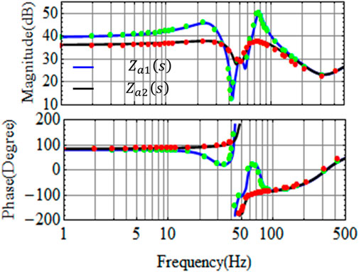
FIGURE 3. Bode diagram of the AC port SISO system model.

The stability analysis of the ports intersecting the envelope line is shown in Figure 4 when the short circuit ratios of the AC grids are 2.1 and the power reference of the system is set to 7.2 MW. The corresponding simulation current waveforms and the spectrum are shown in Figure 5.

FIGURE 4

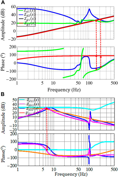
FIGURE 4. Bode diagrams of the SISO input and output models. (A) AC port and (B) DC port.

FIGURE 5

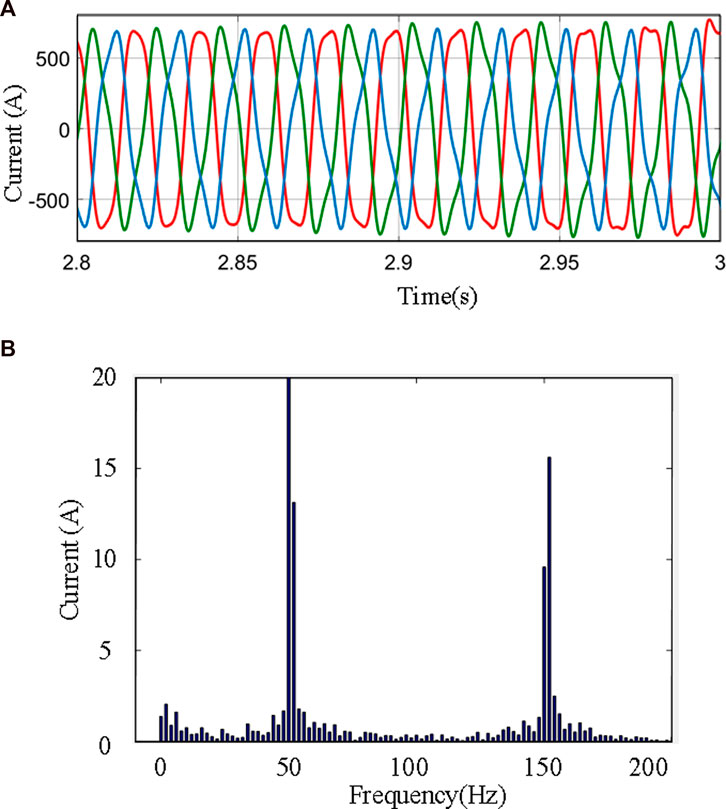
FIGURE 5. Simulation results. (A) AC grid-connected current waveform. (B) Current spectrum.

In Figure 4A, the AC input impedance model of the system based on port A with intersecting envelope lines intersects the impedance of the interconnected power grid at a frequency of 202.8 Hz, and the corresponding phase difference is 130.8°. The phase difference is <180°. The AC input impedance model of the system based on port C with intersecting envelope lines intersects with the impedance of the interconnected power grid at a frequency of 152 Hz, and the corresponding phase difference is 180.6°. The phase difference exceeds 180°, and the system is unstable. In Figure 4B, the equivalent input impedance amplitudes of DC port B are much larger than the output, and there is no amplitude intersection. The equivalent input and output impedance of DC port D intersects at the frequency of 6.3 Hz, and the corresponding phase difference is 74.2°.

The analysis showed that the system is stable only when the impedance ratios of the ports intersecting the envelope line satisfy the Nyquist stability criterion. Therefore, the system is determined to be unstable. Figure 5B shows the spectrum of system simulation waveforms by fast Fourier transform (FFT) in Figure 5A. The spectrum shows that the system has a large amount of harmonics near 152 Hz and 52 Hz, where the system output current oscillates and the system is unstable. This is consistent with the results of the theoretical stability analysis. Therefore, stability analysis based on the ports intersecting the envelope line can reflect the stability of HVDC transmission systems.

4 Key parameter identification and design

Based on the stability analysis of the ports, port C has the smallest stability margin and is the key port that causes instability of the HVDC transmission system. Moreover, the module inverter VSC2 corresponding to AC port C is the key module affecting the system stability. This section discusses the effects of the phase-locked loop and the DC voltage bandwidth on the stability margin of the port.

To intuitively measure the effect of parameters on system stability, the phase margin of the port is defined. In practical engineering, an appropriate phase margin is necessary to ensure the safe and stable operation of the system. The phase margin of the system should be at least 30° in practice (Healey, 1976), (Yang et al., 2021). This paper assumed that the subsystems on both sides of the partition point are stable when running alone. The phase margin ${\mathit{\phi }}_{\mathit{k}}$ of the kth port is defined as

${\phi }_k={180}^0-Abs\left[{\left.\phi {\left[H\right.}_k\left(s_i\right)\right]}_{\left|\left.20\ast \mathit{lg}{\left[H\right.}_k\left(s_i\right)\right]\right.=0}\right],(29)$

where ${\mathit{H}}_{\mathit{k}}\left(\mathit{s}\right)$ is the open-loop gains of the kth port.

Based on the relationship between the control loops of the individual converters and the oscillation interval reported by Sun (2021), the DC voltage control and the PLL are the control parameters causing the oscillation of AC port C. Therefore, the variation in the phase margin of port C with the PLL and the bandwidth of the dc-voltage loop is represented in Figure 6. The upper right corner of Figure 6 is a two-dimensional plane. For port C, the AC phase margin decreases as the DC voltage bandwidth of converter VSC2 and the PLL bandwidth increase. The effect of the PLL bandwidth in converter VSC1 on port C can be neglected.

FIGURE 6

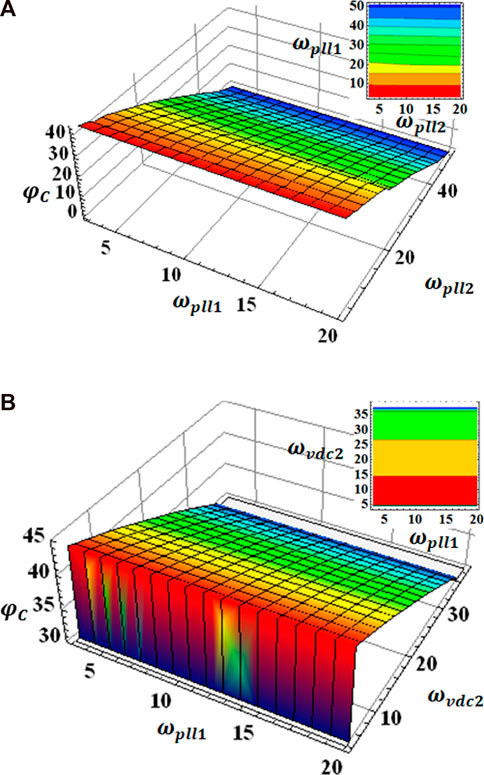
FIGURE 6. Stability margin of port C with different controls. (A) Phase-locked loop. (B) Phase-locked loop and DC voltage loop.

As the PLL bandwidth increases from 5 Hz to 20 Hz in Figure 6A, the stability margin of port C decreases from 43.3° to 30°. As the dc-voltage loop bandwidth increases from 5 Hz to 20 Hz in Figure 6B, the stability margin of port C decreases from 43.4° to 37.2°. Compared to the dc-voltage bandwidth, AC port C is more sensitive to changes in the PLL. Therefore, system stability can be achieved by adjusting the key control PLL bandwidth that affects the stability margin of the system ports.

The stability margin of converter VSC2 port C is 30°, which corresponds to a converter PLL bandwidth of 20 Hz.

If only the stability of the system is considered qualitatively, the range of the PLL bandwidth to guarantee the stability of the system is <50 Hz, and a PLL bandwidth of 45 Hz is chosen.

As the system power increases from 6 MW to 7.2 MW at 2s, the system grid-connected current waveforms under the two parameters are shown in Figure 7. Figure 7A is the dc voltage waveform with a PLL bandwidth of 45 Hz. When the power increases, the dc voltage waveform changes from stable to divergent, and the system is unstable. Figure 7B shows that the dc voltage based on the envelope SISO open-loop gain analysis and design parameters can be rapidly adjusted and can still recover stability after being subjected to voltage perturbations.

FIGURE 7

FIGURE 7. Current simulation waveform with different parameters. (A) Parameter design based on MIMO model analysis. (B) Parameter design based on SISO port analysis.

Compared with the qualitative analysis, the parameters designed based on the quantitative analysis of the envelope SISO open-loop gains can guarantee good system robustness.

5 Conclusion

This study proposed an analysis method for determining the system stability by the SISO open-loop gains. The system is divided by the envelope into sub-modules that are stable when operating individually. Based on the port parameter models of the system, the SISO open-loop gains of the ports were derived. The system stability was analyzed according to the SISO open-loop gains of the ports intersecting the envelope line. The key port and parameters affecting the stability of the system were located based on the stability margin.

Compared with the stability analysis of the single partition point division system, the iterative screening of the zeros and poles of the small feedback loop was avoided. Compared with the qualitative stability analysis, the proposed analysis method can obtain the stability margins of the system and the oscillation frequency band, which can be used to locate the key modules affecting the system stability and to design the parameters. The designed parameters can ensure that the system has good robustness. The results of the stability analysis provide a theoretical basis for system parameter design and network planning. Future studies will further evaluate the application of this stability analysis method in system planning and parameter design.

Data availability statement

The original contributions presented in the study are included in the article/Supplementary Material. Further inquiries can be directed to the corresponding author.

Author contributions

ST conceived the article and edited the manuscript. JL and XD edited the framework and logic of the manuscript. HY edited the introduction and abstract. YC edited the grammar. All authors contributed to the article and approved the submitted version.

Funding

This work was supported in part by the National Natural Science Key Foundation of China (grant 51937001).

Conflict of interest

The authors declare that the research was conducted in the absence of any commercial or financial relationships that could be construed as a potential conflict of interest.

Publisher’s note

All claims expressed in this article are solely those of the authors and do not necessarily represent those of their affiliated organizations, or those of the publisher, the editors, and the reviewers. Any product that may be evaluated in this article, or claim that may be made by its manufacturer, is not guaranteed or endorsed by the publisher.

Supplementary material

The Supplementary Material for this article can be found online at: https://www.frontiersin.org/articles/10.3389/fenrg.2023.1202845/full#supplementary-material

References

Bo, W., Burgos, R., Boroyevich, D., Mattavelli, P., and Shen, Z. (2017). AC stability analysis and DQ frame impedance specifications in power electronics based distributed power systems[J]. IEEE J. Emerg. Sel. Top. Power Electron. (4), 1.

Google Scholar

Cao, W., Ma, Y., and Wang, F. (2017). Sequence-impedance-based harmonic stability analysis and controller parameter design of Three-phase inverter-based multibus AC power systems. IEEE Trans. Power Electron. 32 (10), 7674–7693. doi:10.1109/tpel.2016.2637883

CrossRef Full Text | Google Scholar

Chang, Li, Cao, Yijia, Yang, Yaqian, Wang, L., Blaabjerg, F., and Dragicevic, T. (2021). Impedance-based method for DC stability of VSC-HVDC system with VSG control. Int. J. Electr. Power Energy Syst. 130, 106975. doi:10.1016/j.ijepes.2021.106975

CrossRef Full Text | Google Scholar

Chou, S. -F., Wang, X., and Blaabjerg, F. (2020). Two-port network modeling and stability analysis of grid-connected current-controlled VSCs. IEEE Trans. Power Electron. 35 (4), 3519–3529. doi:10.1109/tpel.2019.2934513

CrossRef Full Text | Google Scholar

Dewangan, L., and Bahirat, H. J. (2020). Controller interaction and stability margins in mixed SCR MMC-based HVDC grid. IEEE Trans. Power Syst. 35 (4), 2835–2846. doi:10.1109/tpwrs.2019.2959066

CrossRef Full Text | Google Scholar

Du, W., Fu, Q., and Wang, H. (2018). Method of open-loop modal analysis for examining the subsynchronous interactions introduced by VSC control in an MTDC/AC system. IEEE Trans. Power Del. 33 (2), 840–850. doi:10.1109/tpwrd.2017.2774811

CrossRef Full Text | Google Scholar

Eto, Y., Noge, Y., Shoyama, M., and Babasaki, T. (2023). Stability analysis of bidirectional dual active bridge converter with input and output LC filters applying power-feedback control. IEEE Trans. Power Electron. 38 (3), 3127–3139. doi:10.1109/tpel.2022.3225113

CrossRef Full Text | Google Scholar

Fan, L., and Miao, Z. (2020). Admittance-based stability analysis: Bode plots, nyquist diagrams or eigenvalue analysis? IEEE Trans. Power Syst. 35 (4), 3312–3315. doi:10.1109/tpwrs.2020.2996014

CrossRef Full Text | Google Scholar

Flourentzou, N., Agelidis, V. G., and Demetriades, G. D. (2009). VSC-based HVDC power transmission systems: An overview. IEEE Trans. Power Electron. 24 (3), 592–602. doi:10.1109/tpel.2008.2008441

CrossRef Full Text | Google Scholar

Healey, Martin (1976). Principles of automatic control. London, UK: The English universities press LTD, 45–78.

Google Scholar

Huang, Y., and Wang, D. (2018). Effect of control-loops interactions on power stability limits of VSC integrated to ac system. IEEE Trans. Power Del. 33 (1), 301–310. doi:10.1109/tpwrd.2017.2740440

CrossRef Full Text | Google Scholar

Liu, F., Liu, J., Zhang, H., and Xue, D. (2014). Stability issues of Z+ Z type cascade system in hybrid energy storage system (HESS). IEEE Trans. Power Electron. 29 (11), 5846–5859. doi:10.1109/tpel.2013.2295259

CrossRef Full Text | Google Scholar

Shah, S., and Parsa, L. (2017). Impedance modeling of three-phase voltage source converters in DQ, sequence, and phasor domains. IEEE Trans. Energy Convers. 32 (3), 1139–1150. doi:10.1109/tec.2017.2698202

CrossRef Full Text | Google Scholar

Sun, J. (2021). Two-port characterization and transfer immittances of AC-DC converters Part I: Modeling[J]. IEEE Open J. Power Electron. (99), 1.

Google Scholar

Sun, J. (2022). Frequency-domain stability criteria for converter-based power systems. IEEE Open J. Power Electron. 3, 222–254. doi:10.1109/ojpel.2022.3155568

CrossRef Full Text | Google Scholar

Sun, J. (2011). Impedance-based stability criterion for grid-connected inverters. IEEE Trans. Power Electron. 26 (11), 3075–3078. doi:10.1109/tpel.2011.2136439

CrossRef Full Text | Google Scholar

Sun, J., Li, M., Zhang, Z., Xu, T., He, J., Wang, H., et al. (2017). Renewable energy transmission by HVDC across the continent: System challenges and opportunities. CSEE J. Power Energy Syst. 3 (4), 353–364. doi:10.17775/cseejpes.2017.01200

CrossRef Full Text | Google Scholar

Tan, S., Du, X., Liu, J., and Zhao, Y. (2020). “Modeling and Stability Analysis of VSC-HVDC System Considering AC/DC dynamic interaction response with frequency coupling,” in Proceedings of the 2020 IEEE 9th International Power Electronics and Motion Control Conference, Nanjing, China, November 2020, 2786–2792.

CrossRef Full Text | Google Scholar

Yang, Z., Chen, T., Luo, X., Schülting, P., and De Doncker, R. W. (2021). Margin balancing control design of three-phase grid-tied PV inverters for stability improvement. IEEE Trans. Power Electron. 36 (9), 10716–10728. doi:10.1109/tpel.2021.3061624

CrossRef Full Text | Google Scholar

Zhang, C., Cai, X., Molinas, M., and Rygg, A. (2019). On the impedance modeling and equivalence of AC/DC-Side stability analysis of a grid-tied type-IV wind turbine system. IEEE Trans. Energy Convers. 34 (2), 1000–1009. doi:10.1109/tec.2018.2866639

CrossRef Full Text | Google Scholar

Zhang, C., Molinas, M., Rygg, A., and Cai, X. (2020). Impedance-based analysis of interconnected power electronics systems: Impedance network modeling and comparative studies of stability criteria. IEEE J. Emerg. Sel. Top. Power Electron. 8 (3), 2520–2533. doi:10.1109/jestpe.2019.2914560

CrossRef Full Text | Google Scholar

Zhang, H., Harnefors, L., Wang, X., Gong, H., and Hasler, J. -P. (2019). Stability analysis of grid-connected voltage-source converters using SISO modeling. IEEE Trans. Power Electron. 34 (8), 8104–8117. doi:10.1109/tpel.2018.2878930

CrossRef Full Text | Google Scholar

Zhang, H., Mehrabankhomartash, M., Saeedifard, M., Zou, Y., Meng, Y., and Wang, X. (2021). Impedance analysis and stabilization of point-to-point HVDC systems based on a hybrid AC–DC impedance model. IEEE Trans. Ind. Electron. 68 (4), 3224–3238. doi:10.1109/tie.2020.2978706

CrossRef Full Text | Google Scholar

Zhu, Y., Zhang, Y., and Green, T. C. (2023). Injection amplitude guidance for impedance measurement in power systems. IEEE Trans. Power Electron. 38 (6), 6929–6933. doi:10.1109/tpel.2023.3256182

CrossRef Full Text | Google Scholar

Zou, X., Du, X., and Wang, G. (2018). “Modeling and stability analysis for multiple parallel grid-connected inverters system,” in Proceedings of the 2018 IEEE Applied Power Electronics Conference and Exposition (APEC), San Antonio, TX, June 2018, 2431–2436.

CrossRef Full Text | Google Scholar