Flexibility resource planning of a power system considering a flexible supply–demand ratio

Aiming at the problems of insufficient power system regulation capacity and lack of flexible resources caused by source-load uncertainty, the flexible resource planning of power systems is studied with the goal of improving flexibility. Uncertainty and flexibility are combined in this article, and a probability index of an insufficiently flexible supply-demand ratio is proposed based on the probability characteristics of flexibility. A bi-level programming model of power system flexibility resources considering the probability of an insufficiently flexible supply demand ratio is constructed. Optimal economics is used as the objective function of the planning layer, and the proposed minimum probability index of the flexible supply-demand ratio is used as the objective function of the operations layer. Economics and flexibility are studied, taking the power system in a certain area in Northeast China as the research object. A flexible resource planning scheme that meets different flexibility expectations is obtained, and the scheme is discussed in detail from the aspects of system flexibility, economic cost, and new energy consumption capacity. The effectiveness of quantitative indicators and planning methods are verified.

Introduction

Under the global low-carbon goal, the penetration of new energy generation is increasing in power systems worldwide (International Energy Agency, 2009). Affected by natural factors, wind and solar power generation bring uncertainty to the system operations, while the load side indeterminacy arises due to the massive access to distributed new energy (State Grid Energy, 2020; Zhang et al., 2020; Guo, 2021). Posed by the requirement of responding to the system uncertainties, flexibility has become one of the most important performance indicators of current and future power systems (Ding et al., 2018; National Development and Reform Commission and the National Energy, 2018). Therefore, to improve the flexibility of power systems, the flexibility quantification method under uncertainty and its application in related planning have become important research directions.

There are many studies on flexibility. The North American Electric Reliability Cooperation (2011) defines the flexibility of power systems as the ability to make full use of system resources to respond to load fluctuations. In International Energy Agency (2008), flexibility is defined as the ability of power systems to respond quickly to foreseeable and unforeseen changes and emergencies in a specific economic operation. Flexibility can be summarized as the ability of the system to respond to uncertain factors, which involves the actual operations and investment planning of a power system. The selection and application of quantitative flexibility indicators are also different for different research objects and research fields. Indicators applicable to the planning problem include the technical flexibility index (T_USFI), the technical and economic flexibility index (TE_USFI), the expected loss of load (LOLE), and the expected energy not supplied (EENS) (Capasso et al., 2005; Li and Wang, 2020; Zhao et al., 2021). It can be seen that the application of system flexibility indicators in power system planning focuses on economics. The indicators applicable to operational problems include the insufficient ramping resource expectation (IRRE), the operational flexibility index (UlBig A), and the expected value of up–down flexibility shortage (Lannoye et al., 2012; Ul Big and Andersson, 2012; Li et al., 2015). In Lu and LiQiao (2018), flexibility is quantified from the demand and the supply side. System uncertainty leads to an increase in demand for flexibility. It is proposed that there are some connections between flexibility and source–load uncertainty. Guo (2020) shows that flexibility quantification has a certain guiding significance for power system flexibility resource planning with large-scale new energy access. The aforementioned quantitative flexibility indicators are mostly focused on the application of traditional power system planning, operations, and other scenarios. Few studies examine the quantitative flexibility indicators that consider uncertainty, and those indicators are not often applied to power systems with increased proportions of new energy sources and dual source–load uncertainty.

For power systems with a large proportion of new energy, there is a mutual restraint relationship between flexibility and economics (Xiao, 2015). There have been some achievements in system planning research considering flexibility. In Yang et al. (2022), a bi-level programming model is adopted. The upper layer is the planning layer, and the lower layer is the operations layer. The planning result is economically optimal, and the flexibility margin is considered the planning layer constraint to participate in the planning. In Li et al. (2021), a transmission network planning model based on flexibility and economics is proposed using a multi-objective programming method, aiming at the optimal investment cost, operating cost, renewable energy abandonment, and flexibility. The optimal solution is obtained by adding the weights of multiple objectives. The lowest flexibility weight does not highlight the system’s requirement for flexibility. In Xu et al. (2019), flexibility adjusts the decision variables in the form of indicators and selects the scheme with the least cost through iteration. Compared with the (k-1)th iteration, in the kth iteration process, when the cost increases, the unit new investment is selected to improve the flexibility index. Cui and Zhang (2018) established a multi-time scale economic dispatch model of photovoltaic units to optimize the flexibility of climbing. In Lu et al. (2019), a wind turbine planning method considering system flexibility and new energy consumption capacity was constructed to maximize the system’s adjustability and enhance the ability to accept new energy.

In summary, the current research on flexibility mostly focuses on the establishment of quantitative flexibility indicators considering economics and proposes evaluation methods, while less research examines quantitative flexibility indicators that consider uncertainty and the application of flexibility indicators in power system planning. In terms of application, most studies are based on the planning and design of the power supply side based on power flexibility, while there are few studies on the planning of flexible resources (Zi, 2018; Yu et al., 2022).

In view of the aforementioned problems, this paper will research quantifying flexibility under uncertainty and propose a probability index of an insufficiently flexible supply–demand ratio based on the probability characteristics of flexibility. A bi-level programming model of power system flexible resources considering the probability of an insufficiently flexible supply–demand ratio is constructed. Optimal economics is used as the objective function of the planning layer, and the proposed minimum probability index of the flexible supply–demand ratio is used as the objective function of the operations layer. Economics and flexibility are studied, taking the power system in a certain area in Northeast China as the research object and verifying the effectiveness of the proposed indicators and models.

Flexibility quantification under system uncertainty

The flexibility of a new power system is its response ability to deal with uncertainty. It is necessary to consider the uncertainty factor in the flexibility index. System uncertainty is frequently neglected in the study of the flexibility quantification index. To strengthen the connection between them, a flexible supply–demand ratio index is proposed by characterizing the adjustment ability of the system to the source–load uncertainties at multiple scales (15 mins, 1 h, 1 day). Based on this, a quantitative index based on the flexibility probability characteristics is defined and named the probability index of an insufficiently flexible supply–demand ratio. The expressions are as follows:

The flexible supply–demand ratio R_fsd characterizes the quantitative relationship between flexible supply and demand in a certain time range. The expression is as follows:

$R_{fsd,i,t}=\frac{{\displaystyle \sum }_{a\in S}{X}_{a,t}}{{\displaystyle \sum }_{b\in D}{Y}_{b,t}}=\frac{{\displaystyle \sum }_{a\in S}{X}_{a,t}}{P_{NL,t}},$

where $R_{fsd,t}$ is the supply–demand ratio of the system in t period under a certain time scale i, S represents the set of flexible supply sources, and X_a,t represents the supply of the ath flexible resource at a certain time scale (MW/t), D represents a collection of flexibility requirements, Y_b,t denotes the bth flexibility demand in t period under a certain time scale (MW/t), and P_NL,t is the net load value of t period under a certain time scale, not less than zero (MW/t). When the supply–demand ratio is equal to 1, the system reaches the balance of supply and demand. If the flexibility margin is considered, the supply–demand ratio must be greater than 1.

The amount of flexibility supply is the sum of the flexibility provided by various flexibility resources of the system at this time. Common flexibility resources include traditional generator sets, new energy generator sets, power-to-hydrogen, and electric vehicles. The number of flexibility requirements is equal to the net load of the system at this time. The net load represents the ability of the system to cope with the insufficient power supply caused by the uncertainty of wind–solar electric field output and the uncertainty of load demand at a certain time scale i. That is, the expression of the system flexibility demand in the tth period is

$P_{NL,i,t}={\displaystyle \sum }_{i\in I}\left(P_{L,i,t}-P_{W,i,t}-P_{S,i,t}\right.),$

where time period t contains i time scales and is the load size in the i time scale. P_L,t is the wind turbine output at the i time scale. P_W,t is the photovoltaic generator output at the i time scale. The probability of an insufficiently flexible supply–demand ratio (P_IFSR-α) is used to characterize the probability that the system flexibility is in short supply. The threshold α represents the flexibility expectation; its physical meaning is the target value set by the system. In the ideal state, the threshold α = 1 indicates that the supply and demand balance is satisfied. The specific expression is as follows:

$P_{IFSR}-\alpha =\mathit{PR}\left(R_{fsd}<\alpha \right)=\mathit{PR}\left(\frac{{\displaystyle \sum }_{a\in S}{X}_{a,t}}{{\displaystyle \sum }_{i\in I}\left(P_{L,i,t}-P_{W,i,t}-P_{S,i,t}\right)}<\alpha \right).$

The process of solving this index is shown in Figure 1. Compared with traditional indicators, its advantages include: 1) Simplifying the quantization process. The initial data processing is simple, and the convolution and volume differences of random variable functions are replaced by the ratio of total supply and demand. 2) Strengthening the link between uncertainty and flexibility. The uncertainty of wind power directly affects the flexibility demand of the system, thus affecting the index value. The threshold value directly represents the ability of the system to deal with uncertain factors. 3) The index can be used to evaluate the flexibility of new power systems under multiple time scales. It can obtain the index through the historical operations data in a short time, check the flexibility of the system immediately, and evaluate the flexibility of the long-term operations of the system using a year’s historical data.

FIGURE 1

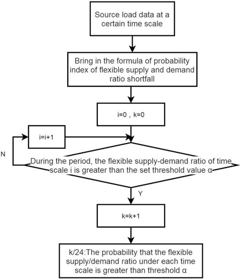
FIGURE 1. The proposed solving process.

Dynamic mathematic model of flexible resources

The adjustment methods used to address the system volatility and uncertainty factors can be used as flexibility resources. Common flexibility resources include traditional generator sets, energy storage, power-to-hydrogen, and electric vehicles. In this paper, three common dynamic response models of flexible resources are established that can be used to calculate the flexibility index or participate in flexible resource planning as the constraint part of the planning model.

Traditional generation units

Traditional flexible resources include thermal power, hydropower, and nuclear power, which account for a large proportion of the overall power structure. Traditional flexible power supply is mainly from thermal power units; the flexibility they provide is as follows:

$\left\{\begin{array}{l}{F}_{ga,u,t}=\min \left\{r_{ga,u}{T}_0,P_{ga,\max }-\left.P_{ga,t}\right\},\right.\\ F_{ga,d,t}=\min \left\{r_{ga,d}{T}_0,P_{ga,t}-\left.P_{ga,\min }\right\},\right.\\ P_{ga,\min }\le P_{ga,t}\le P_{ga,\max },\\ P_{ga,\min }=0.31P_{ga,\max },\end{array}\right.$

where F_ga,u,t and F_ga,d,t are the flexibility of upregulation and downregulation provided by the thermal power units at time t, r_ga,u and r_ga,d are the upward climbing rate and downward climbing rate of the thermal power units, T₀ is the scheduling time of the thermal power units, P_ga,max and P_ga,min are the maximum technical power output and the minimum technical power output of the thermal power units, respectively, and P_ga,t is the active power output of the thermal power units at time t. In order to ensure that flue gas emissions meet the standard, thermal power units should operate stably at more than 31% of their rated capacity.

Power to hydrogen

Power to hydrogen (P2H) is used to consume unbalanced power during low load periods, which is one of the important means of converting power to gas. Compared with the process of power to (natural) gas (P2G), P2H can avoid the energy loss of the methanation reaction. P2H uses redundant new wind and solar energy to generate electricity and then uses that electricity to decompose water into hydrogen and oxygen, which not only avoids the environmental pollution caused by traditional fossil fuel hydrogen production but also alleviates the waste of abandoned wind and light energy. The expression of P2H is as follows:

$V_{P_{2H,t}}=\frac{P_{elc,t}\cdot \Delta t}{{\mu }_h},$

where V_P2H,t is the volume of hydrogen produced by the electrolytic cell in t period, P_elc,t is the average power consumption of the electrolysis cell in t period, ∆t is the length of time period t, and μ_h is electrolysis cell unit power consumption, generally taken as 4.50–5.04 (kw•h/N•m³). The expressions of flexibility and related constraints provided by P2H are as follows:

$\left\{\begin{array}{l}{S}_t=S_{t-1}+P_t^{ch}\cdot {\eta }^{ch}-\frac{P_t^{dis}}{{\eta }^{dis}}-O_t,\\ S^{\min }\le S_t\le S^{\max },\\ F_{P2H,u,t}=P_t^{ch},\\ F_{P2H,d,t}=P_t^{dis},\\ I_t^{ch}\cdot P^{ch,\min }\le P_t^{ch}\le I_t^{ch}\cdot P^{ch,\max },\\ I_t^{dis}\cdot P^{dis,\min }\le P_t^{dis}\le I_t^{dis}\cdot P^{dis,\max },\\ 0\le I_t^{ch}+I_t^{dis}\le 1,\end{array}\right.$

where S_t is the hydrogen storage energy of the hydrogen storage tank in the P2H system during the t period (MWh); F_P2H,u,t and F_P2H,d,t are, respectively, the upward adjustment flexibility and downward adjustment flexibility provided by the P2H system at time t; $P_t^{ch}\mathrm{a}\mathrm{n}\mathrm{d}{P}_t^{dis}$ are the charging power and discharging power of hydrogen energy storage in t period, corresponding to the power of hydrogen production by electrolysis of water and the power of hydrogen power generation in t period, respectively (in MW); ${\eta }_t^{ch}\mathrm{a}\mathrm{n}\mathrm{d}{\eta }_t^{dis}$ are the charging efficiency and discharging efficiency of the system, corresponding to the efficiency of water electrolysis and hydrogen power generation; O_t is the power of hydrogen sold to the hydrogen trading market for other hydrogen industries in period t (MW); S^max and S^min are the upper and lower energy storage limits of the P2H system (in MWh); P^ch,max and P^ch,min are the operating power upper and lower limits of the water electrolysis hydrogen production device (in MW); P^dis,max and P^dis,min are the upper and lower operating power limits of the hydrogen power generation device, respectively (in MW); $I_t^{ch}\mathrm{a}\mathrm{n}\mathrm{d}{I}_t^{dis}$ are the charge–discharge state of the electric-to-hydrogen system in the t period and are binary variables; $I_t^{ch}=1$ indicates that the power-to-hydrogen system is in a charged state during t period; and $I_t^{dis}=0$ is the discharge status.

The economic benefit of hydrogen production is that hydrogen can be sold directly after it is produced using excess wind power. Therefore, the profit value of P2H as a system flexibility resource is considered here, and its expression is as follows:

$C_{elc}={\displaystyle \sum _{t=1}^T}{\lambda }_{H_2}\frac{P_{elc,t}\cdot \Delta t}{{\mu }_h},$

where C_elc is the economic benefit of selling hydrogen and ${\lambda }_{H_2}$ is the selling price of hydrogen per unit volume (2.7 yuan/Nm³).

Energy storage

The charging and discharging response time of energy storage technology is short, usually in seconds. It can provide bilateral flexibility for the power system, such as providing power when the power generation is less than the load or consuming the remaining electricity when the power generation is greater than the load. Energy storage can effectively improve the utilization rate of new energy. The expressions of flexibility and related constraints provided by energy storage are as follows:

$\left\{\begin{array}{l}{F}_{ESS,u,t}=P_{ESS,d,t},\\ F_{ESS,d,t}=P_{ESS,d,t},\\ S_{ESS,\min }\le S_{ESS,t}\le S_{ESS,\max },\\ P_{ESS,d,\min }\le P_{ESS,d,t}\le P_{ESS,d,\max },\\ P_{ESS,c,\min }\le P_{ESS,c,t}\le P_{ESS,c,\max },\end{array}\right.$

where $F_{ESS,u,t}\mathrm{a}\mathrm{n}\mathrm{d}{F}_{ESS,d,t}$ are the upward and downward adjustment flexibilities provided by the energy storage system to the system at time t; $P_{ESS,d,t}\mathrm{a}\mathrm{n}\mathrm{d}{P}_{ESS,c,t}$ are the discharge and charging power of the energy storage system at time t; and $P_{ESS,d,\max }\mathrm{a}\mathrm{n}\mathrm{d}{P}_{ESS,d,\min }$ are the maximum and minimum discharge power of the energy storage system, respectively. $P_{ESS,c,\max }\mathrm{a}\mathrm{n}\mathrm{d}{P}_{ESS,c,\min }$ are the maximum and minimum charging power for the energy storage system. $S_{ESS,t}$ is the state of charge of the energy storage system.

Flexible resource planning model considering a flexible supply–demand ratio

In order to make full use of the value of flexible resources in the power system while considering the economics of the system, a bi-level programming model of power system flexible resources based on the quantitative index of flexibility under uncertainty is proposed by referring to the probability index of an insufficiently flexible supply–demand ratio (P_IFSR-α) proposed previously. The selection scheme of the upper-level decision variables determines the optimization process of the lower-level optimization model. The lower-level optimization model will feed the optimal value to the upper-level optimization model, and the upper level will then calculate the global optimal planning results based on the obtained lower-level optimal value. The bi-level programming model relationship shown in Figure 2 consists of a planning layer model and an operations layer model.

FIGURE 2

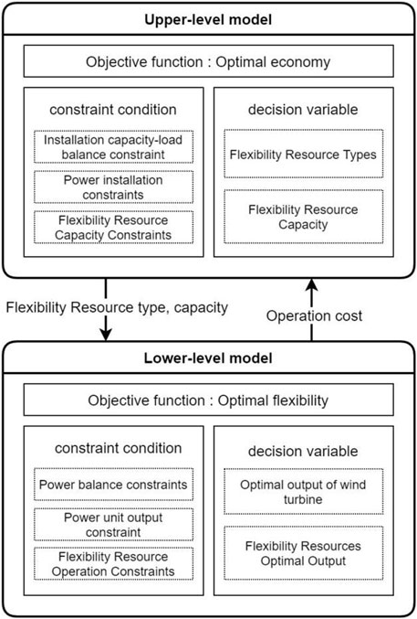
FIGURE 2. The bi-level programming model relationship.

Upper-level programming model

The upper-level programming model takes optimal economics as the goal and the type and capacity of flexible resources as the decision variables. On the basis of satisfying the balance of power and electricity, carbon emission constraints, and flexibility margin constraints, collaborative optimization is carried out with the goal of minimizing the construction cost of new resources and the surplus value of existing resources, and the planning decision scheme is obtained.

Upper programming objective function

The upper-level programming objective function is the most economical; that is, it has the lowest economic cost. The objective function is expressed as follows:

$\min f_1=\min \left(C_{new}+C_{elc}+C_{Fm}+C_{Om}+C_{Fu}+C_{Curt}\right),$

where f₁ is the cost of resource investment decision-making stage, C_new is the cost of new unit investment decision-making stage, C_elc is the profit value cost of new resources, the sum of C_Fm and C_Om is the maintenance cost, C_Fu is the fuel cost, and C_Curt is the penalty cost of wind abandonment.

New resources investment construction cost

The construction cost of new resources is the construction cost of flexible resources, which is expressed as follows:

$C_{\mathrm{n}\mathrm{e}\mathrm{w}}={\displaystyle \sum _{t=1}^T}\left({\displaystyle \sum }_{n\in N}{x}_{n,t}{I}_{n,t}{P}_{n,t}\right)CRF,$

where x_n,t determines whether the flexibility resource is constructed as a 0/1 variable; P_n,t and I_n are the new investment capacity and unit investment cost of the flexible resource n in the fourth year, respectively; N represents the collection of flexibility resources, including flexibility part, energy storage, power-to-hydrogen, and electric vehicles provided by conventional thermal power units; and T is the planning cycle.

$CRF=\frac{\sigma {\left(1+\sigma \right)}^d}{{\left(1+\sigma \right)}^d-1},$

where CRF is the investment cost recovery coefficient, d represents the conversion days of various active resources, and σ represents the discount rate; this paper uses 5%.

Maintenance cost

The maintenance cost can be divided into the fixed equipment maintenance cost and variable operations maintenance cost. The equipment maintenance cost is related to the type and capacity of flexible resources and can be expressed by a certain proportion of the investment cost. The fixed maintenance cost is shown as follows:

$C_{Fm}=\beta C_f^{new},$

where the ratio of the fixed maintenance cost to initial investment cost is 0.03.

$C_{O\mathrm{m}}={\displaystyle \sum _{t=1}^T}{\displaystyle \sum }_{k\in K}{P}_{k,t}{\beta }_k^{Om},$

where P_k,t is the power consumption of each flexible resource at time t and ${\beta }_k^{Om}$ is the operations maintenance cost of each flexible resource per unit of power consumption.

Fuel costs

The fuel cost only considers the coal cost of thermal power units.

$C_{Fu}=C_{coal}{\displaystyle \sum _{t=1}^T}{f}_{g,t},$

where C_coal is the unit coal consumption cost of the thermal power unit. f_g,t is the coal consumption of the thermal power unit at time t, which can be expressed as the secondary form of power generation:

$f_{g,t}=a\cdot {\left(P_{g,t}\right)}^2+b\cdot P_{g,t}+c,$

where a, b, and c are the coal consumption coefficients of thermal power units, and P_g,t is the power generation of the thermal power unit at the moment.

Wind curtailment penalty cost

The penalty cost of wind curtailment is added to the target to increase the consumption rate of wind power:

$C_{Curt}=C_w^{curt}{\displaystyle \sum _{t=1}^T}{P}_{w,t}^{curt},$

where $C_{Curt}$ is the unit wind abandonment penalty cost and $P_{w,t}^{curt}$ is the abandoned wind volume of the wind turbine at the moment, which is equal to the predicted power generation of wind power minus the actual power generation of wind power.

Upper planning constraints

Installation capacity–load balance constraint

${\displaystyle \sum _{m=1}^M}\Delta P_{m,t}+{\displaystyle \sum _{n=1}^N}\Delta P_{n,t}\ge L_t\left(1+R_t\right),$

where P_m,t is the installed capacity of the various power sources in the t year, P_n,t is the installed capacity of the various flexible resources in year t, L_t is the maximum load of the system in year t, and R_t is the capacity reserve coefficient.

Power installation constraints

$\left\{\begin{array}{l}{P}_{m,t}\ge 0,\\ P_{m,t}^{\min }\le P_{m,t}\le P_{m,t}^{\max },\end{array}\right.$

where $P_{m,t}^{\min }$ and $P_{m,t}^{\max }$ are the minimum and maximum installed capacities of various types of hydropower and nuclear power, respectively.

Flexibility resource capacity constraints

$\left\{\begin{array}{l}{P}_{n,t}\ge 0,\\ P_{n,t}^{\min }\le P_{n,t}\le P_{n,t}^{\max },\end{array}\right.$

where $P_{n,t}^{\min }$ and $P_{n,t}^{\max }$ are the lower and upper limits of the installation capacity of various flexible resources in year t, respectively, and are selected according to the actual situation.

Lower-level programming model

The lower-level programming model solves the flexibility problem under uncertainty in the new power system. In upper-level programming, the unit capacity is selected as the decision variable with the goal of economic optimization, the optimal output of various flexible resources satisfying the optimal goal of system flexibility is obtained, and the optimal output curve is obtained as the decision variable of the upper-level programming.

Lower-level programming objective function, aiming at optimal flexibility

$\min f_2=\min P_{IFSR},$

where $f_2$ indicates that the objective function of the lower-level programming model is optimal flexibility. For the flexible supply and demand ratio, $P_{IFSR}$ is used to characterize the system’s ability to adjust supply to meet the demand.

Lower planning constraints

Power balance constraints

$P_{g,t}+P_{w,t}+P_{s,t}+P_{n,t}+P_{h,t}+P_{l,t}=L_t+P_{loss}+P_{f,t},$

where $P_{g,t},P_{w,t},P_{s,t}{,P}_{n,t},P_{h,t},P_{l,t},P_{loss},L_t,P_{f,t}$ are the thermal power units, wind turbines, photovoltaic units, nuclear power units, hydropower units, tie lines, network losses, loads, and flexible resource absorption power in the simulated operating period t, respectively.

Power unit output constraints

${\lambda }_m^{\min }{P}_{m,t}\le P_{m,t}\le {\lambda }_m^{\max }{P}_{m,t},$

where ${\lambda }_m^{\min },{\lambda }_m^{\max },\mathrm{a}\mathrm{n}\mathrm{d}{P}_{m,t}$ represent the minimum and maximum output coefficients of each power unit and the output of the unit at each moment in the operations simulation, respectively.

Flexibility resource operations constraints

$0\le P_{n,t}\le P_{n,t}^{\max },$

where $P_{n,t}^{\max }$ is the maximum flexibility provided by each type of flexibility resource in the t period.

Insufficiently flexible supply–demand ratio probability constraint

In order to ensure sufficient flexibility, the index constraints of the system to meet the flexibility are given.

$P_{IFSR}-\alpha =\mathit{PR}\left(R_{\mathrm{f}\mathrm{s}\mathrm{d}}<\alpha \right)\le P_{IFS{R}_{\max }},$

where $P_{IFS{R}_{\max }}$ is the flexibility evaluation index value when the system flexibility is the worst (1), which indicates that the flexible system supply cannot meet the demand at any time. $\alpha$ is the flexibility expectation that is numerically equal to the flexible supply and demand ratio target value.

System simulation analysis

Base data

The example of this paper takes the power system in a certain area of Northeast China as the research object. The upper layer applies the genetic algorithm; the lower layer calls the fmincon function and uses MATLAB to write a program to solve the model. The new power system includes a total capacity of 1.49456 million kilowatts of thermal power units, 43.5 million kilowatts of wind turbines, 19.1 million kilowatts of photovoltaic units, 12.196 million kilowatts of hydropower units, and 22.3 million kilowatts of nuclear power units. The economic parameters involved in the example are shown in Table 1. The planning layer considers the annual planning cost, the optimization cycle of the operations layer is 24 h, and the time scale is 1 h, ignoring the influence of the unit ramp. The target value of the flexible supply and demand ratio (flexibility expectation α) ranges from 0.6 to 0.9.

TABLE 1

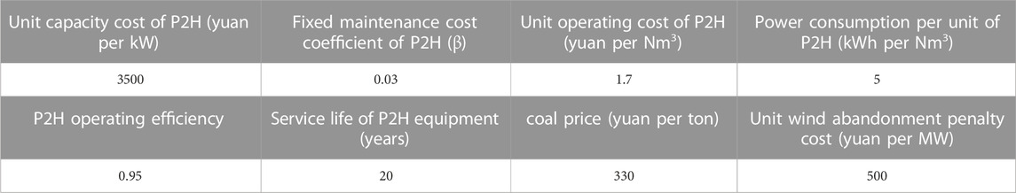
TABLE 1. Flexibility economic parameters for resource planning.

Through the Latin hypercube sampling scene generation and K-means clustering scene reduction method, the uncertainty of the wind power load is processed, and typical days of large wind power–small load, large wind power–large load, small wind power–large load, and small wind power–small load are generated. After clustering, the weights of each typical daily scenario are 0.148, 0.18, 0.219, and 0.677, respectively. The wind abandonment situation is observed on a typical large wind power–small load day. The output and load curve of the system unit is shown in Figure 3. The new energy power generation accounts for approximately 40%, and there is obvious wind abandonment.

FIGURE 3

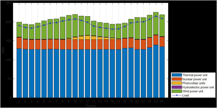
FIGURE 3. The output and load curve of the system unit.

Analysis of simulation results

Through simulation, the optimal flexibility resource planning capacity is obtained when the system meets different flexibility expectations (α) under different uncertainties, taking into account economics and flexibility. The results are shown in Table 2.

TABLE 2

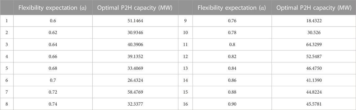
TABLE 2. Flexibility resource planning results under different flexibility expectations.

The aforementioned table shows the planning results of the flexibility resource power-to-hydrogen when the system flexibility expectation threshold is 0.6–0.9. That is, when the system flexibility supply can meet the flexibility demand of 60%–90% as the planning target, considering the economics and flexibility, the optimal power-to-hydrogen capacity is planned. It can be seen that there is no direct linear or non-linear relationship between the capacity of flexibility resources and the expected value of flexibility due to the consideration of economics.

Flexibility analysis

Taking the typical large wind power–small load day as an example, the system flexibility under the planning is analyzed. As shown in Figure 4, under the optimal planning capacity, when the supply-demand ratio of the system is required to be less than 0.68, the probability of an insufficiently flexible supply–demand ratio is 0; that is, the flexibility supply meets the flexibility demand of 68% at any time in the cycle, and the system can fully respond to the flexibility demand caused by uncertainty. When the demand–supply ratio of the system is greater than 0.86, the probability of insufficiently flexible supply and demand is 1; that is, the flexibility supply cannot meet the 86% flexibility demand at any time, and the system does not have the ability to respond to uncertainty. When the threshold is set to 0.7, that is, when the expected system meets 70% flexibility, the flexibility supply–demand ratio is 0.0417; that is, the probability that the system meets the flexibility supply to meet the 70% flexibility demand in the cycle is 4.17%. Compared with the large wind power–small load scenario, the flexibility index is reduced.

FIGURE 4

FIGURE 4. The system flexibility under the planning.

Financial analysis

The simulation data of system planning cost and corresponding flexibility index are shown in Table 3.

TABLE 3

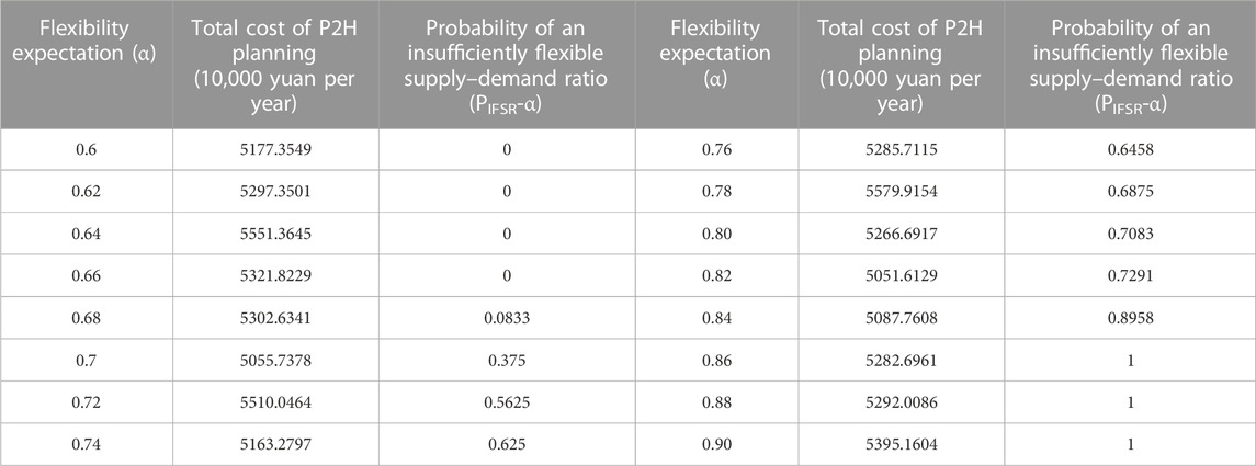
TABLE 3. Annual planning cost and flexibility index evaluation.

In the scenario of large wind power–small load, when the system flexibility is sufficient, that is, in the planning with the probability index of an insufficiently flexible supply and demand ratio of 0, if the optimal economic cost is expected to be the lowest, the power-to-hydrogen planning capacity with the expected flexible supply and demand ratio of 0.6 is selected according to Table 3. In order to achieve optimal flexibility, the corresponding power-to-hydrogen capacity is selected when the flexible supply–demand ratio is 0.66, and the total planned cost is 532.18229 million yuan.

Analysis of new energy consumption

In the large wind power–small load scenario, the P2H capacity with 66% responsiveness of the system to system uncertainty is selected for wind abandonment analysis. From Tables 2, 3, it can be seen that when the expected system flexibility supply meets the 66% flexibility demand at any time, the power-to-hydrogen capacity is 39.1352 MW, and the total planned cost is 53.218229 million yuan per year.

The P2H output during the lower-level operations optimization with flexibility as the only goal and the electricity-to-hydrogen power consumption after the economic flexibility bi-level programming are shown in Table 4. It can be seen from the data in the table that when the flexibility optimization is carried out separately, the total P2H power consumption is 603.8982 MW. After considering the economics and flexibility, the power consumption of P2H increases to 605.0252 MW.

TABLE 4

TABLE 4. P2H power consumption in MW/h for different targets.

This paper only considers “green hydrogen”; that is, the conversion of electricity to hydrogen made from wind curtailment is green hydrogen, and its power consumption is equivalent to the consumption of wind curtailment. The system diagram after flexible resource planning is shown in Figure 5.

FIGURE 5

FIGURE 5. The system diagram after flexible resource planning.

It can be seen intuitively from Figure 5 that flexible resource planning has the benefit of accommodating new energy. After calculation, the typical daily wind abandonment penalty cost before planning is 319,730 yuan. When only considering the flexibility of the system, the wind abandonment penalty cost is reduced to 34,998.3 yuan. After the economic flexibility bi-level planning, it is reduced to 17,217.4 yuan. At the same time, flexible resource planning reduces the operating cost of the new power system and improves the economics of the system.

Conclusion

Aiming at the insufficient response ability and flexibility resources problem caused by uncertainties in both the supply and load sides, research is carried out on improving system flexibility while making full use of the flexible resources in the power system while considering the economics of the system. A probability index of an insufficiently flexible supply–demand ratio with flexibility probability characteristics is proposed to guide flexibility resource planning. A bi-level programming model of power system flexibility resources considering the probability of an insufficiently flexible supply–demand ratio is constructed, taking the power system in a certain area in Northeast China as the research object. The conclusions are as follows.

1) A probability index of an insufficiently flexible supply–demand ratio is proposed. Compared with the traditional flexibility index, it can effectively quantify the flexibility of the power system under the uncertainty of both the power supply side and the load side, strengthen the connection between uncertainty and flexibility, and describe the relationship between flexible supply and demand.

2) A resource planning model of the power system considering a flexible supply and demand relationship is constructed that takes into account economics and flexibility. By using the probability index of an insufficiently flexible supply–demand ratio, the flexibility expectation of the planning scheme can be selected, and the optimal scheme can be obtained by combining the evaluation results of planning cost and flexibility index. This scheme will not lead to poor economics in order to ensure ultra-high flexibility, nor will it force the system to not respond to operational risks in order to achieve optimal economics. The planning results can safely and effectively improve the new energy consumption capacity of the system.

Data availability statement

The original contributions presented in the study are included in the article/Supplementary Material; further inquiries can be directed to the corresponding author.

Author contributions

Conceptualization, XZ and ML; methodology, HL; software, FG; validation, CZ, XZ, and ML; resources, HL; data curation, FG; writing—original draft preparation, CZ; writing—review and editing, XZ; visualization, ML; supervision, HL. All authors contributed to the article and approved the submitted version.

Funding

This work was supported by the Science and Technology Project of State Grid Liaoning Electric Power Co., Ltd. (No. 2022YF-62).

Acknowledgments

The authors would like to thank the School of Electric Power, Shenyang Institute of Engineering, for helpful discussions on topics related to this work.

Conflict of interest

Authors XZ, ML, HL, FG, and CZ were employed by State Grid Liaoning Economic Research Institute.

The remaining author declare that the research was conducted in the absence of any commercial or financial relationships that could be construed as a potential conflict of interest.

The authors declare that this study received funding from the Science and Technology Project of State Grid Liaoning Electric Power Co., Ltd. (No.2022YF-62). The funder was involved in the study design, collection and analysis.

Publisher’s note

All claims expressed in this article are solely those of the authors and do not necessarily represent those of their affiliated organizations, or those of the publisher, the editors, and the reviewers. Any product that may be evaluated in this article, or claim that may be made by its manufacturer, is not guaranteed or endorsed by the publisher.

References

Capasso, A., Falvo, M. C., and Lamedica, R. (2005). “A new methodology for power systems flexibility evaluation[C],” in 2005 IEEE Russia Power Tech Conference, St. Petersburg, Russia, 27-30 June 2005 (IEEE), 27–30.

Google Scholar

Cui, M., and Zhang, J. (2018). Estimating ramping requirements with solar-friendly flexible ramping product in multi-timescale power system operations. Appl. Energy 225 (1), 27–41. doi:10.1016/j.apenergy.2018.05.031

CrossRef Full Text | Google Scholar

Ding, Y., Shao, C., and Yan, J. (2018). Economical flexibility options for integrating fluctuating wind energy in power systems: The case of China. Appl. Energy 228, 426–436. doi:10.1016/j.apenergy.2018.06.066

CrossRef Full Text | Google Scholar

Guo, J. B. (2021). Challenges faced by new power systems and thinking on related mechanisms[J]. China Power Enterp. Manag. 25, 8–11. doi:10.3969/j.issn.1671-735X.2021.12.028

CrossRef Full Text | Google Scholar

Guo, T. (2020). Power system flexibility evaluation and flexibility transformation planning research[D]. Beijing: North China Electric Power University.

Google Scholar

International Energy Agency (2008). Empowering variable renewables-options for flexible electricity flexible electricity systems[R]. Internatio Energy Agency.

Google Scholar

International Energy Agency (2009). Empowering Variable Renewables—Options for Flexible Electricity Systems: (Complete Edition)[J]. OECD Energy 23, 1—36.

Google Scholar

Lannoye, E., Flynn, D., and O'Malley, M. (2012). “Assessment of power system flexibility: A high-level approach[C],” in 2012 IEEE Power and Energy Society General Meeting, San Diego, CA, USA, 22-26 July 2012 (IEEE).

Google Scholar

Li, H., Lu, Z., and Qiao, Y. (2015). Evaluation of power system operation flexibility with large-scale wind power integration[J]. Power grid Technol. 39 (6), 1672–1678. doi:10.13335/j.1000-3673.pst.2015.06.032

CrossRef Full Text | Google Scholar

Li, L. F., Chen, Z. P., Hu, Y., Tai, N. L., Gao, M. P., and Zhu, T. (2021). Renewable energy power system expansion planning based on flexibility and economy[J]. J. Shanghai Jiao Tong Univ. 55 (07), 791–801. doi:10.16183/j.cnki.jsjtu.2020.024

CrossRef Full Text | Google Scholar

Li, W. N., and Wang, Q. (2020). Stochastic production simulation for generating capacity reliability evaluation in power systems with high renewable penetration. Energy Convers. Econ. 1 (3), 210–220. doi:10.1049/enc2.12016

CrossRef Full Text | Google Scholar

Lu, Y., WuChen, S. Y. J. Z., Liu, J., and Kang, C. Q. (2019). A planning method for wind power and photovoltaic absorption considering flexible resources[J]. Distrib. Energy 4 (05), 10–16. doi:10.16513/j.2096-2185.DE.191089

CrossRef Full Text | Google Scholar

Lu, Z., and LiQiao, H. Y. (2018). Probabilistic flexibility evaluation for power system planning considering its association with renewable power curtailment. IEEE Trans. Power Syst. 33 (03), 3285–3295. doi:10.1109/tpwrs.2018.2810091

CrossRef Full Text | Google Scholar

National Development and Reform Commission and the National Energy (2018). Guidance on improving the regulation capacity of power system. Energy Res. Util. 10, 3.

Google Scholar

North American Electric Reliability Cooperation (2011). North American Electric Reliability Corporation 1, hereby submits this Notice of Filing of[J].

Google Scholar

State Grid Energy (2020). Research Institute Co Ltd [M].Beijing: China Electric Power Press.

Google Scholar

Ul Big, A., and Andersson, G. (2012). “On operational flexibility in power systems[C],” in Proceedings of the Power and Energy Society General Meeting, San Diego California, USA, 22-26 July 2012 (IEEE), 22–26.

Google Scholar

Xiao, D. Y. (2015). Research on flexibility evaluation index and optimization of power system with large-scale renewable energy[D]. Shanghai: Shanghai Jiaotong University.

Google Scholar

Xu, T. H., Lu, Z. X., Qiao, Y., and An, J. (2019). Source-load-storage multi-type flexible resource coordinated high-proportion renewable energy power planning[J]. Glob. Energy Internet 2 (01), 27–34.

Google Scholar

Yang, J., Li, F. T., and Zhang, G. H. (2022). New energy high permeability system planning method considering flexibility requirements[J]. Power Grid Technol. 46 (06), 2171–2182. doi:10.13335/j.1000-3673.pst.2021.0943

CrossRef Full Text | Google Scholar

Yu, D., Guo, Y. H., Wu, J., Li, J. T., and Wang, C. M. (2022). Flexibility improvement planning and evaluation of regional integrated energy system considering uncertainty[J]. Power Supply 39 (04), 84–92. doi:10.19421/j.cnki.1006-6357.2022.04.012

CrossRef Full Text | Google Scholar

Zhang, Y. Z., Dai, H. C., and Zhang, N. (2020). The low-carbon transformation of power system needs ' multi-line attack ' [N]. Beijing: China Energy News.

Google Scholar

Zhao, S., Xu, M., and Zhou, W. (2021). Simulation of sequential operation of multi-energy power system considering section constraints[J]. Electr. Power Autom. Equip. 41 (07), 1–6. doi:10.16081/j.epae.202104011

CrossRef Full Text | Google Scholar

Zi, P. L. (2018). An extreme scenario method for robust transmission expansion planning with wind power uncertainty[J]. Energies 11, 8. doi:10.3390/en11082116

CrossRef Full Text | Google Scholar