 Rongqiang Feng1,2
 Tianchi Du
 Wei Ding
- 1NARI Group (State Grid Electric Power Research Institute) Co., Ltd., Nanjing, China
- 2NARI-TECH Nanjing Control Systems Co., Ltd., Nanjing, China
- 3College of Energy and Electrical Engineering, Hohai University, Nanjing, China
- 4Shandong Computer Science Center (National Supercomputer Center in Jinan), Qilu University of Technology (Shandong Academy of Sciences), Jinan, China
The integration of a high proportion of wind power has brought disorderly impacts on the stability of the power system. Accurate wind power forecasting technology is the foundation for achieving wind power dispatchability. To improve the stability of the power system after the high proportion of wind power integration, this paper proposes a steady-state deduction method for the power system based on large-scale wind power cluster power forecasting. First, a wind power cluster reorganization method based on an improved DBSCAN algorithm is designed to fully use the spatial correlation of wind resources in small-scale wind power groups. Second, to extract the temporal evolution characteristics of wind power data, the traditional GRU network is improved based on the Huber loss function, and a wind power cluster power prediction model based on the improved GRU network is constructed to output ultra-short-term power prediction results for each wind sub-cluster. Finally, the wind power integration stability index is defined to evaluate the reliability of the prediction results and further realize the steady-state deduction of the power system after wind power integration. Experimental analysis is conducted on 18 wind power farms in a province of China, and the simulation results show that the RMSE of the proposed method is only 0.0869 and the probability of extreme error events is low, which has an important reference value for the stability evaluation of large-scale wind power cluster integration.
1 Introduction
With the proposal of the “carbon peaking and carbon neutrality” goal, the utilization of new energy for power generation has been elevated to a crucial strategic position (Wang et al., 2021). Wind power utilization has a dual nature: on the one hand, its lack of pollution and renewable nature make it more economically efficient from the perspective of generation cost. On the other hand, the inherent intermittency, randomness, and uncertainty of wind power make it difficult for power systems to schedule and affect the stable operation of the power system (Kazari et al., 2018; Mostafaeipour et al., 2022). The high penetration of wind power, in particular, significantly increases the uncertainty of power grid operation. If wind power is not accurately grasped and reasonably used, it will reduce the economy and safety of power grid operation. Wind power forecasting technology is one of the key technologies for realizing wind power utilization. The ultra-short-term wind power cluster forecasting method provides wind power forecasting results for the subsequent 4 h, which provide technical reference for dispatchers to arrange unit combinations and formulate power generation plans. For large-scale wind power clusters, accurate wind power forecasting technology can improve the absorption of wind power, increase the power system’s grasping ability for wind power, and thereby enhance the stability of the power system after wind power is connected to the grid (Ju et al., 2019).
The current main ultra-short-term wind power cluster forecasting methods are divided into two categories: physical model and data-driven (Wu et al., 2020). The physical model method is highly dependent on atmospheric physical characteristics and requires support from a large amount of meteorological observation data. If the mathematical description of the wind power farm is accurate enough, the prediction accuracy is often high. However, the performance of the prediction will be seriously affected when the wind power farm is expanded or the mechanical characteristics change (Dolatabadi et al., 2021). Data-driven methods include support vector machines (Li et al., 2020), extreme learning machines (ELMs) (Wan et al., 2020), and neural networks (Nazir et al., 2020; Tang et al., 2022), which have made significant breakthroughs in prediction accuracy compared with physical prediction methods.
With the application of new generations of artificial intelligence algorithms and the proposals of improvement methods such as combined models and switching mechanisms, the prediction accuracy of a single power prediction algorithm has gradually improved (Carneiro et al., 2022). However, China’s wind power development is transitioning from decentralized to centralized and large-scale, and wind power farms are mostly connected to the grid in a centralized manner. It is beneficial to improve wind power prediction accuracy by using the smoothing effect presented by the aggregation of wind power farms and promoting wind power consumption. Therefore, wind power cluster prediction has become extremely important (Mu et al., 2022).
For wind power cluster prediction methods, the principle of superposition is relatively simple, which obtains the cluster power prediction result by adding single-site power predictions and is suitable for sparsely distributed and small-scale wind power farms (Zong and Porté-Agel, 2020). The time-series extrapolation method analyzes historical power data to predict future trends in time series. As meteorological data are not sufficiently introduced, they are significantly affected by the quality of power data. The statistical upscaling method only needs to linearly upscale the predicted output of the reference wind power farm to obtain the cluster prediction result. This method can offset potential correlation factors between different wind power farms’ data and has good dynamic adaptability, but the selection criteria for the reference wind power farms are difficult to determine (Yang et al., 2022). The cluster division method divides the wind power farms in the region into several wind sub-clusters according to the fluctuation patterns of power and meteorological data and establishes a separate prediction model for each sub-cluster.
The division of wind power clusters is generally based on the spatio-temporal characteristics of meteorological and power data as inputs, which are partitioned into finite cluster units through clustering or other similarity measures. Predictive models are established for each cluster unit separately. Wang et al. (2022) used wind power as the input for a fuzzy clustering algorithm to achieve cluster division. Zhao et al. (2021) clustered the fluctuations of wind power and considered numerical weather prediction (NWP) meteorological features for short-term wind power forecasting. Abedinia et al. (2020) divided clusters by determining the correlation of output features through empirical orthogonal functions. Fan et al. (2020) proposed using NWP information of the predicted period as input for cluster division. These references used wind power, wind speed, and their constructed attributes as features for clustering, but a single feature’s input may not guarantee the rationality of cluster division when there are quality issues in the data.
The current research on power prediction for large-scale wind power clusters lacks consideration for the stability of wind power integration. Under the condition of a high frequency of extreme errors and inflated overall prediction accuracy, the rationality of the application of prediction results cannot be guaranteed. Additionally, the rationality of cluster division also has a major impact on prediction accuracy. Based on the previously mentioned analysis, a wind power cluster ultra-short-term power prediction method is proposed to consider the stability of wind power integration. Based on the stability evaluation results, further implementation of the power system steady-state deduction is recommended after the wind power grid connection is achieved. A multi-dimensional input feature construction and an improved DBSCAN (density-based spatial clustering of applications with noise) algorithm-based wind power cluster division scheme are proposed, which divide the wind power farms in the region into several subsets. Then, the gated neural unit is improved to extract the temporal features of the wind power cluster and provide the cluster power prediction results. Finally, a stability evaluation index is constructed to assess the reliability of the wind power prediction model, and the effectiveness of the proposed method is verified in 18 wind farms in a province in northeast China.
This paper is organized as follows: Section 2 improves the DBSCAN algorithm and its clustering of wind farm groups. The wind power cluster forecasting model based on the improved GRU network is introduced in detail in Section 3. Section 4 describes the framework for steady-state power system analysis based on large-scale wind power clusters. The effectiveness of the proposed method is verified in Section 5 based on actual wind farm data. Finally, conclusions and future recommendations are presented in Section 6.
2 Wind power subset cluster division based on the improved DBSCAN algorithm
2.1 Improved DBSCAN algorithm
DBSCAN is one of the most typical density-based spatial clustering algorithms, which clusters samples with high similarity in the form of partitioning clusters, and clusters are defined as the largest set of density-connected points (Mao et al., 2021). Therefore, the DBSCAN algorithm can divide regions with sufficient data density into clusters and is less sensitive to noisy data. The partitioning idea of wind power clusters based on the DBSCAN algorithm is as follows. Input indicates that the status of all input samples is marked as unclustered, an input sample is read, and then the sample is judged as a core sample point according to the neighborhood
Definition 1. The neighborhood
where
Definition 2. For
Definition 3. Given data space
where, Eq. 3 presents that
Definition 4. Given data space
Definition 5. Given data space

FIGURE 1. Flowchart of the improved DBSCAN algorithm.
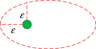
FIGURE 2. Diagram of the core sample search area.
2.2 Clustering of wind power cluster sub-regions based on the DBSCAN algorithm
The input features are a key factor affecting the output of cluster algorithms. Since cluster algorithms generally perform feature engineering separately, the paper characterizes the meteorological and power fluctuation characteristics of each wind power farm by manually constructing features. Salazar et al. (2022) pointed out that hub-height wind speed and power fluctuations in NWP are far more correlated than other meteorological attributes; so, wind speed is one of the key constructed features. Using a 1-h observation window, the variance between the wind speed and the average wind speed in the observation window is extracted to describe the wind speed fluctuations, as shown in Eq. 5.
where
Similarly, the power variability within the 1-h observation window is calculated using Eq. 5 as the second constructed feature. The trend of wind speed quantification within the 1-h observation window is shown in Eq. 6.
where
Similarly, the power change trend within the 1-h observation window is obtained by Eq. 5 as the fourth structural feature. Finally, a structural feature set is formed by
3 Wind power cluster prediction model based on the improved GRU network
GRU is a simplified variation of the LSTM network, which is a kind of gate recurrent unit network and is widely used in extracting time-series features of time series. The update gate in the GRU is a combination of the forget gate and the input gate in the LSTM network, but the GRU model structure is simpler, which effectively reduces the training time while ensuring the model prediction accuracy (Qu et al., 2021; Xiao et al., 2023). The internal structure of the GRU is shown in Figure 3.
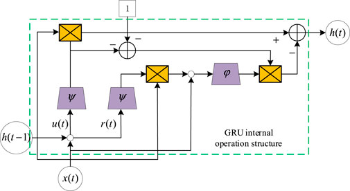
FIGURE 3. GRU neural network structure.
Each GRU includes an
where
During the training stage, in order to reduce the sensitivity of the model to abnormal data, the gradient update of the deep neural network decreases with the decrease of the error, which is conducive to speeding up the convergence speed, and the Huber loss function is used as the measurement rule of the GRU network training loss (Tang et al., 2021). The principle is as follows.
where
According to the wind power cluster division results, the wind power farm data in each sub-cluster are fused with spatial data. Taking a cluster containing

FIGURE 4. Spatio-temporal feature data structure.
4 Framework for steady-state power system analysis based on large-scale wind power cluster forecasting
The traditional modeling approach for wind power cluster forecasting is to first predict the power of each individual wind power farm and then add up the predicted results to obtain the forecasted power of the entire wind power cluster (Wu et al., 2021; Ning et al., 2023). The rationale for this approach is that the prediction units for individual wind power farms are relatively small, and each wind power farm has relatively complete historical data. Achieving high prediction accuracy for each wind power farm will lead to higher accuracy for the regional wind power cluster forecast. Based on this advantage, all the current provincial-level wind power cluster power forecasts use this modeling method.
However, historical power analysis of individual wind power farms shows that the high-frequency components of wind power fluctuate more violently, reducing the predictability of wind power. The randomness and volatility caused by such local effects are difficult to reflect in NWP, making it difficult for prediction models to extract such fluctuation characteristics. However, within a certain spatial range, wind power farms with similar output can smooth out this random fluctuation to some extent, resulting in a smoother aggregated power curve and improved predictability.
Based on the aforementioned analysis, dividing wind power farms in a region into several clusters and modeling them separately can improve the prediction accuracy for each cluster, thereby improving wind power forecasting accuracy and enhancing the stability of power system operation after wind power integration. The steady-state extrapolation framework for power systems based on the forecast results of large-scale wind power clusters is shown in Figure 5.
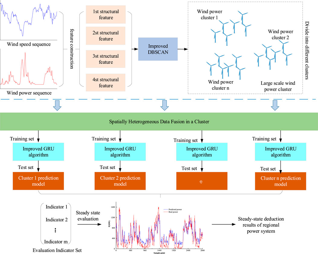
FIGURE 5. Power system stability assessment framework.
The establishment of this framework involves the following three steps:
i) Partitioning wind power sub-clusters: the DBSCAN algorithm was improved based on Eqs 1–4, features were constructed representing the fluctuation characteristics of wind power speed and wind power according to Eqs 5, 6, they were used as inputs for the improved DBSCAN algorithm, and the wind power farms in the region were partitioned into several clusters.
ii) Ultra-short-term power prediction for wind power clusters: the data were merged within the same wind power cluster, spatial data tensors were constructed, the improved GRU neural network was used to extract the temporal characteristics of the wind power cluster, and the wind power cluster forecast was output.
iii) Steady-state deduction of power systems: stability evaluation indicators for wind power prediction were constructed, the stability and accuracy of the wind power prediction model were evaluated comprehensively based on traditional wind power error indicators, and the steady-state deduction of power systems was further realized.
5 Experimental analysis
5.1 Dataset and prediction metrics
The data used in this study consist of 6 months (January to July) of actual power generation data and corresponding NWP data with 15-min resolutions from 18 wind power farms located in northeast China with a total installed capacity of 2,564.81 MW. The meteorological variables included in the NWP dataset are wind speed, temperature, humidity, and pressure. Wind direction was not included as a feature in this study. The first 6 months of data were used as the training set, and the last month data were used as the testing set. To ensure fairness in evaluating the correlation between each feature variable and power, both the NWP features and power were normalized to the [0, 1] range using the normalization algorithm shown in Eq. 12.
where
To reduce the impact of abnormal data on prediction accuracy (Dong et al., 2023), the following pre-processing steps were taken:
1) Power values exceeding the installed capacity were reassigned to the installed capacity;
2) Negative power values were set to zero;
3) For time points where the power is zero, the corresponding wind speed value was set to zero.
The deep learning network designed in this paper consists of three GRU network layers with 16, 32, and 16 neurons, respectively. The last GRU layer is connected with a fully connected layer, and the 16-step wind power prediction results are directly output. The training parameters are as follows: {epoch:50, batch_size: 128, droup_out:0.2}. This paper uses a CPU for training, and the parameters of the computer are as follows: {CPU: Intel(R) Core(TM) i5-7300HQ CPU @ 2.50 GHz 2.50 GHz, RAM: 16.0 GB}.
The loss curve modeled by Cluster 1 is shown in Figure 6. MSE loss declines slowly, with oscillations occurring in the middle of the process, while Huber loss declines faster and has a more stable downward trend.
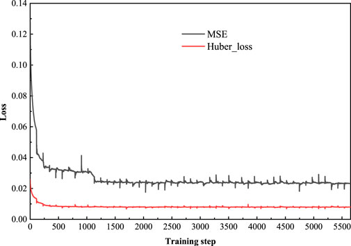
FIGURE 6. Loss curve.
In the past, the index for ultra-short-term wind power prediction often selected the average forecast value within 4 h. However, in the “Technical Regulation for Wind Power Prediction,” the assessment has been modified to the fourth hour, namely, the results of the 16th step of the prediction (Demolli et al., 2019). Therefore, in this study, the normalized root mean square error (RMSE) and normalized maximum absolute error (MAE) were used as the final evaluation criteria to evaluate the performance of the 16th-step prediction (Zhao et al., 2022).
The calculation of normalized RMSE is shown in Eq. 14:
where
The calculation of normalized MAE is shown in Eq. 15:
In addition, the extreme error frequency (SA) index was established to evaluate the stability of the wind power prediction model, using 40% of the installed capacity as the threshold for extreme errors. The calculation is shown in Eq. 16:
where
The calculation of the extreme error bandwidth ratio (EWR) of wind power prediction results is shown in Eq. 17:
During the assessment period, if the extreme error frequency is less than 4% and the normalized RMSE is less than 15% of the installed capacity, it is considered that the power system meets the static stability requirements during long-term operation. If the extreme error bandwidth gradually increases in the 1–16 step prediction results for the next 1–4 h and remains below 40% of the error bandwidth, then it is considered that the power system is in dynamic stability within the next 4 h from the forecast time. It should be noted that the perspective of the power system steady-state deduction in this study starts from the perspective of the power grid and evaluates its impact on the power system after being connected to the grid based on the comprehensive indicators of wind power prediction. High prediction accuracy and stable model performance are required to ensure the stable operation of the power system after connection. If the model performance is unstable, regardless of the overall accuracy during the assessment period, stable operation of the power system cannot be guaranteed.
5.2 Analysis of cluster results
The iteration number of the clustering algorithm was set to 50 times, with a cluster quantity of 3. The final clustering results of each cluster and the relative positions of each wind power farm are shown in Figure 7:
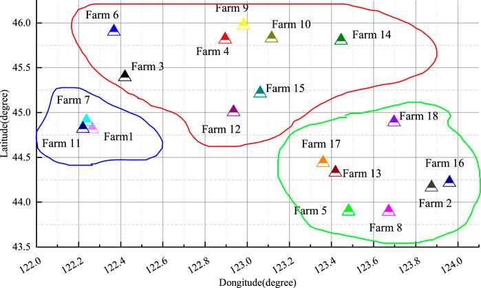
FIGURE 7. Cluster partitioning results.
Cluster 1: including 7 wind power farms, namely, Wind Power Farms 2, 5, 8, 13, 16, 17, and 18.
Cluster 2: including 8 wind power farms, namely, Wind Power Farms 3, 4, 6, 9, 10, 12, 14, and 15.
Cluster 3: including 3 wind power farms, namely, Wind Power Farms 1, 7, and 11.
The cluster results show that the improved DBSCAN algorithm can effectively identify spatially adjacent wind power farm and group them into the same cluster. This indicates the rationality of using the improved DBSCAN algorithm for cluster analysis.
To further verify the rationality of the clusters’ division, a visualization analysis was conducted on the normalized power and wind speed of the wind power farms in Cluster 1. The correlation coefficient matrix of the power output of each wind power farm is also provided, as shown in Figure 8. (Note: Wind Power Farms 1, 7, and 11 are close to each other and share the same NWP data). The correlation coefficient (I) is calculated as shown in Eq. 18.

FIGURE 8. Visualization of Cluster 1 partitioning results. (A) Power output curve of Cluster 1. (B) Wind speed curve of Cluster 1. (C) Correlation coefficient matrix of power output for each wind farm.
Based on the analysis of the previous figure, after cluster division, the power outputs of various wind power farms within the same cluster have certain similarities. Strictly speaking, wind power farms’ output values that are close in distance should exhibit highly similar states. However, during the wind turbine climbing phase between sampling points 192 and 384, there are also differences in power output curves between different wind power farms. Due to factors such as unit maintenance, malfunctions, and power limitations, the relationship between wind power farms’ output and single-unit output is not strictly linearly proportional. Therefore, from the correlation coefficient matrix perspective, the correlation coefficients among the power outputs of various wind power farms within the same wind power cluster do not uniformly maintain high values. For example, the power correlation coefficient between wind power farm 13 and wind power farm 18 is only 0.56. From the analysis of wind speed curves, wind speed trends among the various clusters of wind power farms are relatively similar. Thus, introducing wind speed fluctuation characteristics in clustering features can reduce errors caused by using pure power features.
The normalized power and wind speed, and the correlation coefficient matrix of the normalized power output, for each wind power farm in Clusters 2 and 3 are presented in Figure 9.

FIGURE 9. Visualization of division results of Clusters 2 and 3. (A) Power output curve of Cluster 2. (B) Wind speed curve of Cluster 2. (C) Power output curve of Cluster 3. (D) Wind speed curve of Cluster 3. (E) Correlation coefficient matrix of Cluster 2. (F) Correlation coefficient matrix of Cluster 3.
5.3 Analysis of wind power cluster prediction results
The normalized RMSE and MAE indicators of the three clusters’ power predictions are shown in Figure 10. The normalized RMSE and MAE indicators for Cluster 1 are 0.1018 and 0.0796, respectively; for Cluster 2, they are 0.0602 and 0.1050, respectively; and for Cluster 3, they are 0.0272 and 0.0914, respectively. The prediction RMSE and MAE indicators for all three clusters do not exceed 10% of the installed capacity, indicating that the wind power cluster prediction model proposed in this paper has high prediction accuracy.
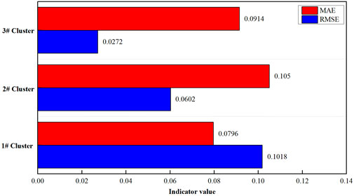
FIGURE 10. Prediction indicators of Clusters 1, 2, and 3.
To further verify the performance of wind power cluster power prediction, the test set prediction results for each of the three clusters were visualized. Figure 11 shows the results of the 16th step of ultra-short-term prediction, where the predicted curve is still able to track the actual power curve very well. It should be noted that predicting wind power at the cluster level cannot overcome the time delay problem that exists in single-farm prediction. That is, there is a notable time delay between the predicted power sequence and the actual power sequence on the waveform. By shifting the predicted sequence forward according to the prediction step, its fluctuation trend almost coincides with the actual power. Due to the presence of the time delay problem, the prediction results for high-power points tend to be lower, while those for low-power points tend to be higher in the overall prediction results. Cluster 1 has a lower installed capacity and thus more high-frequency noise signals in its power, making it difficult to weaken fluctuations through convergence effects. In contrast, Clusters 2 and 3 have higher installed capacities, resulting in better tracking of the actual power curves and higher prediction accuracy than Cluster 1.

FIGURE 11. Visualization of cluster prediction results. (A) Prediction results for Cluster 1. (B) Prediction results for Cluster 2. (C) Prediction results for Cluster 3.
The prediction results for the entire region are shown in Figure 12, where the prediction results for the three wind power clusters are combined to obtain the prediction results for the entire region’s wind power farms. The RMSE is 0.0869, and the MAE is 0.094. The mean absolute error is approximately equal to 10% of the installed capacity, indicating that the model’s performance accuracy can be guaranteed.
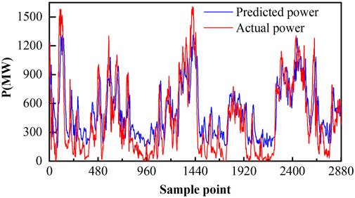
FIGURE 12. Visualization of regional prediction results.
We offer a comparison of several different prediction models, including DBSCAN_LSTM(D_LSTM), DBSCAN_CNN(D_CNN), KMeans_LSTM(K_LSTM), KMeans_GRU(K_GRU), and the persistence method. The comparison index is the normalized RMSE of wind power forecast in the future 4 h. The comparison results are shown in Figure 13. For the prediction of the future 4 h, the error of the model proposed in this paper is the lowest. Among them, the KMeans algorithm has a poor effect on cluster division, and LSTM has poor performance in predicting cluster wind power compared with GRUs; baseline persistence method of time series prediction has the worst predictive performance.
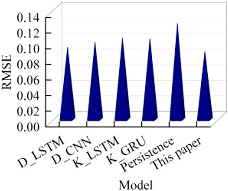
FIGURE 13. Performance comparison of different algorithms.
In addition, we compared the other two prediction patterns. Pattern 1: power prediction is carried out separately for all wind farms, and the final results are added to get the regional power forecast sum. Pattern 2: the total power of the region is taken as the prediction target, and the power prediction results of 4 h are directly output. The performance of the comparison is RMSE in the 4 h; the comparison results are shown in Figure 14. Compared with the other two patterns, the prediction model proposed in this paper has the lowest prediction error.
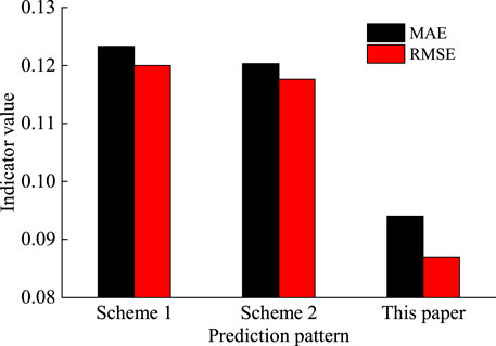
FIGURE 14. Performance comparison of different prediction patterns.
5.4 Analysis of steady-state power system analysis results for a regional grid
During the 1-month assessment period, a total of 59 extreme errors occurred in the wind power clusters in the region, with a frequency of 2.048%, which is not higher than the required 4%. Thus, the large-scale wind power cluster ultra-short-term wind power prediction method proposed in this paper can satisfy the static stability requirements of the power system.
The extreme error bandwidth ratio and the percentage of extreme errors at each prediction step to the extreme error bandwidth for 16-step wind power prediction during the assessment period are shown in Figure 15. The extreme error bandwidth for 16-step prediction gradually increases, but the upward trend is not significant for future steps 7, 8, and 9, indicating that the model proposed in this paper can suppress extreme errors as the prediction step increases. At the 16th prediction step, the proportion of extreme errors is 34.0546%. This result suggests that, under the stable evaluation system proposed in this paper, the wind power prediction accuracy of the wind power cluster in the region can meet the requirements, ensuring stable operation of the power system after grid connection.
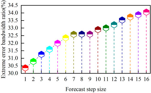
FIGURE 15. Extreme error bandwidth ratio for 16-step prediction.
6 Conclusion
The proposed power system steady-state deduction method, based on the reliability of large-scale wind power cluster power prediction, has improved the stability of power system operation after mass wind power grid connection. The conclusions are as follows:
(1) The improved DBSCAN algorithm can effectively divide wind power clusters based on the constructed wind speed and wind power fluctuation characteristics. The divided wind power clusters have relatively similar actual distances and similar actual power outputs.
(2) The ultra-short-term wind power cluster power prediction method based on the improved GRU algorithm can achieve high prediction accuracy with an RMSE for the fourth hour prediction below 10% of the installed capacity and stable model performance.
(3) Under the power system stability evaluation system constructed in this paper, the proposed ultra-short-term wind power prediction model can effectively improve the operation stability of the power system after a wind power grid connection, with a narrow extreme error bandwidth and a low frequency of extreme errors during the assessment period occurring below 4%.
The next step of this work will further improve the power system stability evaluation indicators and comprehensively evaluate the performance of wind power prediction models from both the grid and generation sides, analyzing their impact on the stable operation of power systems after the wind power grid connection.
Data availability statement
The original contributions presented in the study are included in the article/Supplementary Material; further inquiries can be directed to the corresponding author.
Author contributions
RF designed this study. HY contributed to the improved DBSCAN algorithm. XW contributed to the wind power cluster sub-region clustering method based on DBSCAN. CH contributed to the wind power cluster prediction model based on the improved GRU network. WD performed the framework for steady-state power system analysis based on large-scale wind power cluster forecasting. TD collected and cleansed the data. All authors contributed to the writing of the article, and all agreed to the submitted version of the article.
Funding
This paper was supported by the NARI group science and technology project (grant number: 524609220149).
Conflict of interest
Authors RF, HY, XW, and CH were employed by NARI Group (State Grid Electric Power Research Institute) Co., Ltd. and NARI-TECH Nanjing Control Systems Co., Ltd.
The remaining authors declare that the research was conducted in the absence of any commercial or financial relationships that could be construed as a potential conflict of interest.
The authors declare that this study received funding from the NARI group. The funder had the following involvement in the study: collection, analysis, interpretation of data.
Publisher’s note
All claims expressed in this article are solely those of the authors and do not necessarily represent those of their affiliated organizations, or those of the publisher, the editors, and the reviewers. Any product that may be evaluated in this article, or claim that may be made by its manufacturer, is not guaranteed or endorsed by the publisher.
References
Abedinia, O., Lotfi, M., Bagheri, M., Sobhani, B., Shafie-Khah, M., and Catalão, J. P. (2020). Improved EMD-based complex prediction model for wind power forecasting. IEEE Trans. Sustain. Energy 11 (4), 2790–2802. doi:10.1109/TSTE.2020.2976038
Carneiro, T. C., de Carvalho, P. C. M., Alves dos Santos, H., Lima, M. A. F. B., and Braga, A. P. D. S. (2022). Review on photovoltaic power and solar resource forecasting: Current status and trends. J. Sol. Energy Eng. 144 (1). doi:10.1115/1.4051652
Demolli, H., Dokuz, A. S., Ecemis, A., and Gokcek, M. (2019). Wind power forecasting based on daily wind speed data using machine learning algorithms. Energy Convers. Manag. 198, 111823. doi:10.1016/j.enconman.2019.111823
Dolatabadi, A., Abdeltawab, H., and Mohamed, Y. A. R. I. (2021). Deep spatial-temporal 2-D CNN-blstm model for ultrashort-term LiDAR-assisted wind turbine's power and fatigue load forecasting. IEEE Trans. Industrial Inf. 18 (4), 2342–2353. doi:10.1109/TII.2021.3097716
Dong, X., Ning, X., Xu, J., Yu, L., Li, W., and Zhang, L. (2023). PFAS contamination: Pathway from communication to behavioral outcomes. IEEE Trans. Comput. Soc. Syst. 2023, 1–13. doi:10.1080/10810730.2023.2193144
Fan, H., Zhang, X., Mei, S., Chen, K., and Chen, X. (2020). M2gsnet: Multi-modal multi-task graph spatiotemporal network for ultra-short-term wind farm cluster power prediction. Appl. Sci. 10 (21), 7915. doi:10.3390/app10217915
Ju, Y., Sun, G., Chen, Q., Zhang, M., Zhu, H., and Rehman, M. U. (2019). A model combining convolutional neural network and LightGBM algorithm for ultra-short-term wind power forecasting. Ieee Access 7, 28309–28318. doi:10.1109/ACCESS.2019.2901920
Kazari, H., Oraee, H., and Pal, B. C. (2018). Assessing the effect of wind farm layout on energy storage requirement for power fluctuation mitigation. IEEE Trans. Sustain. Energy 10 (2), 558–568. doi:10.1109/TSTE.2018.2837060
Li, L. L., Zhao, X., Tseng, M. L., and Tan, R. R. (2020). Short-term wind power forecasting based on support vector machine with improved dragonfly algorithm. J. Clean. Prod. 242, 118447. doi:10.1016/j.jclepro.2019.118447
Mao, Y., Mwakapesa, D. S., Xu, K., Lei, C., Liu, Y., and Zhang, M. (2021). Comparison of wave-cluster and DBSCAN algorithms for landslide susceptibility assessment. Environ. Earth Sci. 80, 734–814. doi:10.1007/s12665-021-09896-w
Mostafaeipour, A., Bidokhti, A., Fakhrzad, M. B., Sadegheih, A., and Mehrjerdi, Y. Z. (2022). A new model for the use of renewable electricity to reduce carbon dioxide emissions. Energy 238, 121602. doi:10.1016/j.energy.2021.121602
Mu, G., Wu, F., Zhang, X., Fu, Z., and Xiao, B. (2022). Analytic mechanism for the cumulative effect of wind power fluctuations from single wind farm to wind farm cluster. CSEE J. Power Energy Syst. 8 (5), 1290–1301. doi:10.17775/CSEEJPES.2022.00300
Nazir, M. S., Alturise, F., Alshmrany, S., Nazir, H. M. J., Bilal, M., Abdalla, A. N., et al. (2020). Wind generation forecasting methods and proliferation of artificial neural network: A review of five years research trend. Sustainability 12 (9), 3778. doi:10.3390/su12093778
Ning, X., Tian, W., He, F., Bai, X., Sun, L., and Li, W. (2023). Hyper-sausage coverage function neuron model and learning algorithm for image classification. Pattern Recognit. 136, 109216. doi:10.1016/j.patcog.2022.109216
Qu, Z., Li, M., Zhang, Z., Cui, M., and Zhou, Y. (2021). Dynamic optimization method of transmission line parameters based on grey support vector regression. Front. Energy Res. 9, 634207. doi:10.3389/fenrg.2021.634207
Salazar, A. A., Che, Y., Zheng, J., and Xiao, F. (2022). Multivariable neural network to postprocess short-term, hub-height wind forecasts. Energy Sci. Eng. 10 (7), 2561–2575. doi:10.1002/ese3.928
Tang, G., Gao, X., and Chen, Z. (2022). Learning semantic representation on visual attribute graph for person re-identification and beyond. ACM Trans. Multimedia Comput. Commun. Appl. 2022, 3487044. doi:10.1145/3487044
Tang, G., Gao, X., Chen, Z., and Zhong, H. (2021). Unsupervised adversarial domain adaptation with similarity diffusion for person re-identification. Neurocomputing 442, 337–347. doi:10.1016/j.neucom.2020.12.008
Wan, C., Zhao, C., and Song, Y. (2020). Chance constrained extreme learning machine for nonparametric prediction intervals of wind power generation. IEEE Trans. Power Syst. 35 (5), 3869–3884. doi:10.1109/TPWRS.2020.2986282
Wang, Y., Guo, C. H., Chen, X. J., Jia, L. Q., Guo, X. N., Chen, R. S., et al. (2021). Carbon peak and carbon neutrality in China: Goals, implementation path and prospects. China Geol. 4 (4), 720–746. doi:10.31035/cg2021083
Wang, Y., Wang, J., Cao, M., Li, W., Yuan, L., and Wang, N. (2022). Prediction method of wind farm power generation capacity based on feature clustering and correlation analysis. Electr. Power Syst. Res. 212, 108634. doi:10.1016/j.epsr.2022.108634
Wu, X., Shen, X., Zhang, J., and Zhang, Y. (2021). A wind energy prediction scheme combining cauchy variation and reverse learning strategy. Adv. Electr. Comput. Eng. 21 (4), 3–10. doi:10.4316/AECE.2021.04001
Wu, Z., Xia, X., Xiao, L., and Liu, Y. (2020). Combined model with secondary decomposition-model selection and sample selection for multi-step wind power forecasting. Appl. Energy 261, 114345. doi:10.1016/j.apenergy.2019.114345
Xiao, Y., Zou, C., Chi, H., and Fang, R. (2023). Boosted GRU model for short-term forecasting of wind power with feature-weighted principal component analysis. Energy 267, 126503. doi:10.1016/j.energy.2022.126503
Yang, M., Yan, Q., Dai, B., Chen, X., Ma, M., and Su, X. (2022). An improved spatial upscaling method for producing day-ahead power forecasts for wind farm clusters. IET Generation, Transm. Distribution 16 (19), 3860–3873. doi:10.1049/gtd2.12569
Zhao, J., Guo, Z., Guo, Y., Lin, W., and Zhu, W. (2021). A self-organizing forecast of day-ahead wind speed: Selective ensemble strategy based on numerical weather predictions. Energy 218, 119509. doi:10.1016/j.energy.2020.119509
Zhao, M., Wang, Y., Wang, X., Chang, J., Zhou, Y., and Liu, T. (2022). Modeling and simulation of large-scale wind power base output considering the clustering characteristics and correlation of wind farms. Front. Energy Res. 10, 237–243. doi:10.19746/j.cnki.issn.1009-2137.2022.01.040
Keywords: large-scale wind power cluster, stability assessment, steady deduction, cluster division, ultra-short-term power cluster forecasting, improved GRU
Citation: Feng R, Yu H, Wu X, Huang C, Du T and Ding W (2023) Steady-state deduction methods of a power system based on the prediction of large-scale wind power clusters. Front. Energy Res. 11:1194415. doi: 10.3389/fenrg.2023.1194415
Received: 27 March 2023; Accepted: 13 April 2023;
Published: 09 May 2023.
Edited by:
Xin Ning, Chinese Academy of Sciences (CAS), ChinaReviewed by:
Arghya Datta, Amazon, United StatesAditya Kumar Sahu, Amrita Vishwa Vidyapeetham University, India
Yao Liang, City University of Hong Kong, Hong Kong SAR, China
Lia Elena Aciu, Transilvania University of Brașov, Romania
Xiyun Yang, North China Electric Power University, China
Copyright © 2023 Feng, Yu, Wu, Huang, Du and Ding. This is an open-access article distributed under the terms of the Creative Commons Attribution License (CC BY). The use, distribution or reproduction in other forums is permitted, provided the original author(s) and the copyright owner(s) are credited and that the original publication in this journal is cited, in accordance with accepted academic practice. No use, distribution or reproduction is permitted which does not comply with these terms.
*Correspondence: Wei Ding, ZGluZ3dAc2Rhcy5vcmc=