Thermal performance of three horizontal ground heat exchanger systems: comparison of linear-loop, spiral-coil and slinky-coil arrangements

Ground source heat pumps (GSHPs) are highly efficient for heating and cooling buildings. Among the different types of ground source heat pumps, horizontal ground heat exchangers (HGHEs) gaining popularity due to their cost-effectiveness, ease of installation and high regeneration capacity. However, studies on the interaction and influence of the local environment with the HGHE and the thermal performance influenced by the arrangement and performance of the HGHE are insufficient. This study uses a three-dimensional numerical model to simulate three types of HGHEs, including linear-loop, spiral-coil, and slinky-coil arrangements. Instead of just one unit, three units are connected in series or parallel. The model considers the energy balance and the heat transfer and exchange processes between the heat exchanger and the soil. Simulation of cooling and heating for 1 year revealed that the slinky-coil arrangement is the most affected by heat fluxes at the ground surface, because of its maximum length, which leads to its lowest coefficient of performance (COP) value. The thermal performance of linear-loop and spiral-coil arrangements is similar, but considering the material cost, the linear-coil arrangement has the lowest installation cost and operating cost for 30 years.

1 Introduction

Conventional energy sources, such as oil, natural gas, and coal, are nonrenewable and release harmful environmental pollutants. This lack of sustainability and rising prices has resulted in significant attention and development on renewable and clean energy sources as alternatives to fossil fuels. Among these renewable energy sources, geothermal energy has gathered much interest due to its stability and constancy, environmental friendliness, and high energy efficiency. Compared to deep geothermal energy, shallow geothermal energy is widely used because it is easier to access, requires less cost and effort to install, and is less risky. The development and utilization of shallow geothermal energy is growing rapidly over the past few decades, with exponential growth in heat delivery (Rybach, 2022).

Shallow geothermal energy is based on ground source heat pump (GSHP) systems that regulate the ground as a heat source or sink to condition residential or commercial buildings. GSHP systems can be either in heating or cooling mode by extracting heat from the ground to the building or by absorbing heat from the building and transferring it to the ground through a ground heat exchanger (GHE). Shallow GSHP systems are considered semi-permanent energy sources, having a lifetime of about 40–50 years. Depending on the installation orientation, GHEs can be divided into two main configurations. The first configuration is horizontal ground heat exchangers (HGHEs). HGHEs are usually enclosed and buried in trenches with horizontally installed pipes 1–3 m below the ground surface or in nearby water bodies, such as ponds or lakes. The second configuration is vertical ground heat exchangers (VGHEs) installed in one or more boreholes at a depth of 70–130 m (Hou et al., 2022). VGHEs have higher energy efficiency and heat exchange rates than HGHEs and require less installation area. However, installation costs are much higher depending on the drilling and grouting requirements, and local consent may be needed in most countries. Therefore, HGHEs are more suitable for small-scale buildings and houses with lower energy demand. Nonetheless, unlike VGHEs, HGHEs can be strongly influenced by weather conditions as well as the mass and heat exchange and transfer that occurs at the ground surface in the unsaturated and saturated zones. Prior to installation, HGHEs must be carefully designed and optimized, which can be achieved through numerical modeling, resulting in substantial savings in capital investment. A numerical model used to access the thermal performance of a HGHE usually consists of at least two components: a heat exchanger and its surrounding soil.

Several factors affect the thermal performance of HGHEs, including geometry and arrangement of the pipe, installation and burial depth, and flow rate and working fluid in the pipe. The three most common geometries and arrangements are linear loops, spiral coils, and slinky coils (Aydın et al., 2015). Spiral and slinky coils are more spatially efficient than linear loops. Previous studies in numerical models and experiments have shown that spiral coils performed better than the other two types for the same land area and trench length due to the larger heat exchange area and volume (Congedo et al., 2012; Dasare and Saha, 2015; Yoon et al., 2015; Kim et al., 2016). Coil pitch and diameter, the space between pipes, as well as the pipe material, can also contribute to the thermal performance. It was found that steel and copper pipes have a higher energy efficiency than high-density polyethylene pipes (Selamat et al., 2016; Cao et al., 2017). In contrast, numerical studies have shown that installation depth does not play an essential role on the system performance (Congedo et al., 2012; Dasare and Saha, 2015). The working fluid in most HGHEs operates at a constant flow rate. In general, increasing the flow rate can enhance the performance of HGHEs (Go et al., 2016), but may consume more power for the circulation pump. As an alternative, Zhou et al. (2022) proposed two variable flowrate regulation methods to improve thermal performance and reduce power wastage according to diurnal and seasonal variations in building loads. To prevent working fluids from freezing in low temperature environments, antifreezes are added to the water, such as glycerol. However, Casasso and Sethi (2014) found that calcium chloride (20%) solution performs better than other fluids carrying antifreeze.

The hydrogeological and thermal properties of the surrounding soil are crucial for the heat transfer between the pipe and the ground. The determinant parameter for heat transfer is the soil thermal conductivity. Based on in situ experiments, Naylor et al. (2015) found that fluctuations in soil moisture can cause large variation in soil thermal conductivity. The increment of soil moisture can increase its thermal conductivity and the heat transfer rate of the heat exchanger (Liu et al., 2020). However, moisture transfer is often neglected in most numerical studies (Li et al., 2012a; Kupiec et al., 2015; Kim et al., 2016; Sofyan et al., 2016; Zhou et al., 2022) because it is challenging to obtain spatial information on soil texture and its intrinsic permeability, as well as to simulate phase transitions due to temperature fluctuations caused by the complicated interactions between the atmosphere, ground, and heat exchanger. Numerical simulations by Gan (2018) showed the maximum discrepancies of heat transfer between models with and without moisture transfer through HGHE were 24%, 17%, and 18% in clayey sandy soil, loess sandy soil, and sandy soil, respectively. The source or sink of moisture transfer can result from rain infiltration, topsoil evaporation and soil freezing/thawing, and vegetation evapotranspiration (ET). These processes can be affected by meteorological records and groundwater seepage. Gan. (2013) found that soil freezing increased the heat extraction rate of a HGHE. Go et al. (2016) showed that rain filtration can increase the thermal efficiency of a helical-coil HGHE buried in the unsaturated zone. Shang et al. (2019) in their model that topsoil evaporation and wind speed affected the moisture transfer and caused a lower heat transfer rate. In addition, groundwater flow in saturated soils can also enhance the performance of HGHEs (Li et al., 2018; Shi et al., 2022b). While researchers have developed models that include the interaction of groundwater seepage, soil freezing, and moisture transfer (Meng et al., 2021; Zhang et al., 2021), comprehensive models that consider evaporation and condensation-induced phase changes occurring in the unsaturated and saturated zones, ET in soil-vegetation systems, and diffusion and effusion of moisture in different soil materials have not been developed. However, detailed studies that fully consider evaporation and condensation-induced phase changes occurring in the unsaturated and saturated zones, ET in soil-vegetation systems, and diffusion and effusion of moisture in different soil materials are inadequate.

Soil thermal conductivity is influenced by soil temperature and by the many thermodynamic processes at the ground surface, including short- and long-wave radiation, heat convection and conduction, sensible and latent heat transfer, and heat transfer between the ground and HGHE. These processes can result in a nonuniform distribution of soil thermal conductivity, even if the soil has constant intrinsic properties. However, taking the effect of seasonal variations in soil temperature into account is a challenge. The use of constant or independent functions of surface temperature boundaries in HGHE simulations is insufficient (Li et al., 2012b; Habibi and Hakkaki-Fard, 2018; Sangi and Müller, 2018), especially for the long-term performance of HGHEs. Until now, several researchers have integrated complex energy balance processes into their simulations considering dynamic interactions, including at least one or more thermal processes. Li et al. (2019) found that the thermal performance of a HGHE can vary significantly under constant temperature and energy balance assumptions, especially when the building load is high and the burial depth of the HGHE is shallower than 2.5 m.

For most studies the hydrothermal properties of the ground are assumed to be constant (Go et al., 2016; Tang and Nowamooz, 2019; Zhou et al., 2022). Conversely, the main soil heterogeneity is thought to come from the backfill material, and the effect of different excavated trench backfill materials on thermal conductivity and heat transfer rates were investigated by several researchers. Instead of using the original soil, the encapsulated phase change materials (PCMs) were proposed by Bottarelli et al. (2015). GHE with a mixture of soil and encapsulated PCM was proven to have higher surface temperatures in winter than without PCM, and conversely, lower in summer. Similarly, Al-Ameen et al. (2018) found that replacing Leighton buzzard sand with ground copper slag as a backfill material could also improve the performance of HGHE.

To date, more research is still needed for the numerical simulation of HGHE systems, including 1) energy balance processes should be considered, and different thermal processes should be fully coupled in the simulation; 2) ET from different types of vegetation should be included; and 3) the connection of multiple pipes refers to a more realistic configuration rather than only one loop or one unit of coils. Some recent studies still focus on only one loop or one unit of coils (Zou et al., 2021; Shi et al., 2022a), and do not consider energy transfer through ET of different vegetation. Therefore, this study aims to consider all relevant energy balance processes and to have a better understanding of the effects of diurnal and seasonal variations in ground temperature distributions, as well as their impacts on the thermal performance of variable configurations of HGHEs. The connection of multiple pipes refers to a more realistic configuration rather than only one loop or one unit of coils. We first present the conceptual and mathematical models for the working fluid in a HGHE system and the ground. Sequentially, a three-dimensional model of such a system is constructed to simulate 1-year heating-cooling circulations for a small house. The model incorporates meteorological data measured from a real field site and evaluates their effect on heat transfer, as well as the thermal performance of the HGHE system. At the end, the implications of the model and its potential for the design and optimization of GSHP systems are discussed.

2 Materials and methods

2.1 Energy equation of the fluid in HGHE and the soil

A GSHP usually contains three components, the ground heat exchanger (GHE), heat pump and the building. Three heat transfer mechanisms exist for a GHE and its surrounding soil, including heat conduction, heat convection, and thermal radiation. Heat conduction is the transfer of heat due to thermal gradient, with no mass movement. Heat convection is the transfer of heat through a moving medium (wind or water flow). For GSHP systems, mass transfer can occur between several hydrological and hydrogeological processes, including all weather processes (e.g., precipitation, snow, etc.) and the transport of water from/to the subsurface and vegetation, contributing to the water balance. Water transport processes are complex due to phase transition and mixing processes. For instance, in summer, the liquid phase may become a gas phase due to evaporation, while in winter, there is the possibility of snow and frost events, and then the gas and liquid phases may be transferred to a solid phase. Thermal radiation is caused by electromagnetic radiation. Figure 1 illustrates all the hydrothermal processes that can occur in a buried HGHE system. The mass balance of the soil includes different mass transfer processes, e.g., precipitation and evaporation, infiltration, and evapotranspiration. Along with the mass balance, there is also a heat balance. The heat balance of the soil is determined by the heat capacity, the thermal conductivity, and the atmospheric heat fluxes, including short-wave radiation from the sun and long-wave radiation from the surface and atmosphere (Robinson et al., 2008). Latent heat and sensible heat are absorbed or released in the atmosphere during the heat transfer and balance processes. The HGHE is buried in the soil and extracts or rejects heat from the surrounding soil, and the heat extraction or rejection rate depends on the soil thermodynamic properties and pipe properties, such as pipe geometry and arrangement, the material of the pipe wall, and the flow rate of the circulating fluid in the pipe. In the heating mode, the extracted heat is then transferred to a building through a heat pump, together with the energy input from its compressor. In the cooling mode, the heat generated from the building and the energy input from the compressor are moved to the ground by the heat pump and HGHE.

FIGURE 1

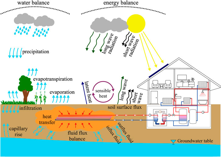
FIGURE 1. Interaction of underground heat exchanger with surrounding soil and environments and different processes of heat and mass transfer occurred in the surface and ground.

The consideration of the heat balance is essential to simulate and evaluate the thermal performance of the HGHE. Here we simply divide the entire HGHE model system into two parts: 1) the pipes of the GHE, and 2) the surrounding soil. Several assumptions we made for the pipes are summarized below.

• Simulation system is used for both heating and cooling of a hypothetical individual house.

• Heat transfer across the cross section is neglected.

• Flow rate of the circulating fluid in the pipes should be well controlled at a constant rate when the heat and circulation pumps are operating.

• Working fluid is water and a small amount of antifreeze, which has the same physical properties as water.

• Diameter of the pipe and its thermal properties are constant.

The assumptions for the surrounding soil are as follows.

• Soil is homogeneous and isotropic under an unconfined condition.

• Heat convection in the soil is neglected.

• Only heat conduction is simulated in the ground.

• Local thermodynamic equilibrium exists between different phases.

Based on the above assumptions the governing equation of the working fluid inside the HGHE pipes and the energy equation of the soil are presented in Eqs 1, 2, respectively.

${\rho }_f{A}_p{C}_{pf}\frac{\partial T_f}{\partial t}+{\rho }_f{A}_p{C}_{pf}\mathbf{u}\bullet \nabla T_f={A_{p}k}_f\nabla \bullet \left(\nabla T_f\right)+\frac{1}{2}{f}_D\frac{{\rho }_f{A}_p}{d_h}{\left|\mathbf{u}\right|}^2+Q_{wall}(1)$

${\rho }_s{C}_{ps}\frac{\partial T_s}{\partial t}-\nabla \bullet \left({\lambda }_s\nabla T_s\right)=-Q_{wall}(2)$

In Eqs 1, 2, T, ρ, C_p, and λ are the temperature, density, specific heat capacity and thermal conductivity, respectively. The subscript f and s indicate the working fluid inside the HGHE and surrounding soil. k_f and u is the conductivity and flow velocity of the working fluid, and A_p, d_h and f_D are the cross-section area, hydraulic diameter (i.e., pipe inner diameter), and friction losses of the pipe. Q_wall is the heat transfer between the working fluid and the ground through the pipe wall. Q_wall is highly dependent on the pipe shape and thickness, as well as the thermal conductivity of the pipe. Values of these parameters are summarized in Table 1. Thermal conductivity of the ground λ_g is affected by many different factors, including saturation, dry density, particle size, gradation, mineralogical composition, packing geometry, temperature, and particle bonding. In natural conditions, soil saturation generally ranges between 0.2–0.7 for most heterogeneous near-surface soil types, and its value of unsaturated soil composed of sand, silt and clay ranges between 0.9–1.2 W/(mK) (Ahmad et al., 2021). The moisture transfer and soil heterogeneity will also affect the thermal performance of the heat exchanger, especially for sand and gravel type where saturation changes quite fast. A moderate value of 1 W/(mK) is given here as the moisture transfer and saturation changes are not integrated in the model.

TABLE 1

TABLE 1. List of model parameters.

2.2 Dimensions and parameters of the heat exchanger and ground

Figure 2 illustrates the configuration of the three-dimensional model used to simulate the performance of three different arrangements of heat exchangers. The model has dimensions of 30 m × 15 m × 10 m with a small box-like area (10.5 m × 7 m × 1.5 m) in the middle representing the trench excavated for the placement of the heat exchangers. Three types of HGHEs are placed in the trench, and their bottoms are all located 1.5 m below the surface of the model, i.e., they are buried at the same depth.

FIGURE 2

FIGURE 2. Model domain and boundaries.

Figure 3 shows the detailed geometry and connections of the HGHEs. The HGHEs are assumed to occupy the same volume as the trench, therefore, the entire length (L) and width (W) of the heat exchanger, as well as the coil diameters of the spiral and slinky tubes (d_coil), are the same as the width of a linear loop (w). The coil pitch defined in Figures 3B, C are the same for spiral- and slinky-coil arrangements, which is half of the coil diameter. The inlet and outlet of the three arrangements are at the same positions, and distance between them (d_i,o) is set to 0.5 m. Center-to-center distance between two units (d) is 2 m for all three cases. Detailed values of these geometric parameters can be found in Table 1.

FIGURE 3

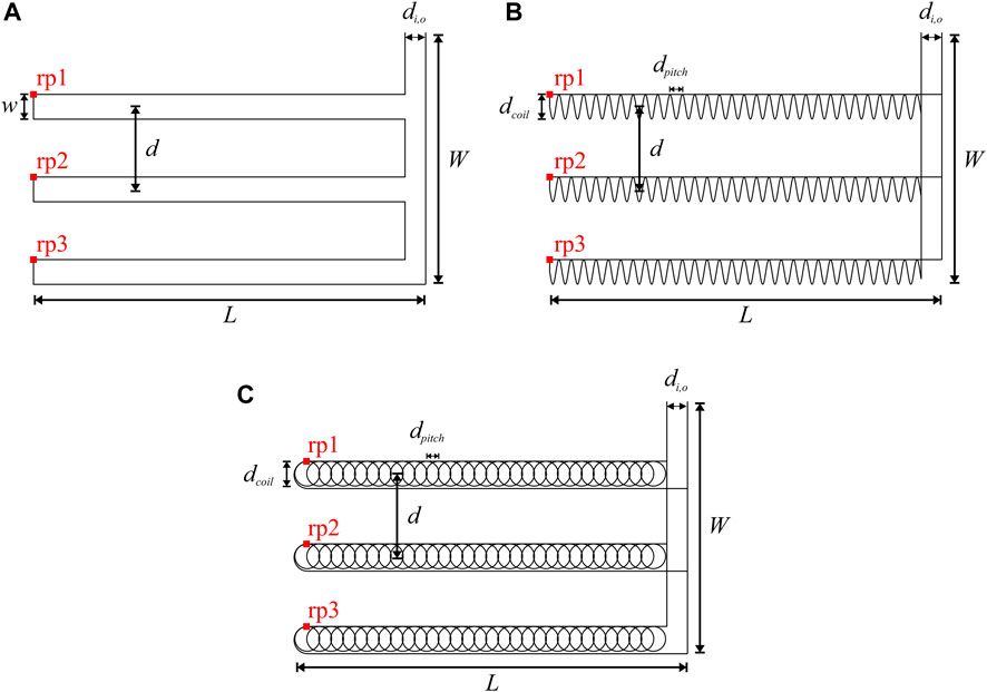
FIGURE 3. Geometry and dimensions of three different heat exchangers. (A) linear-loop; (B) spiral-coil; (C) slinky-coil. Values of the geometric parameters are listed in Table 1.

2.3 Initial and boundary conditions, simulation sequence

The initial conditions of the soil and heat exchanger are assumed to be a constant temperature of 7°C. The four side boundaries of the model are assumed to be at a constant temperature of 7°C and the bottom of the model is a no-flow boundary. The temperature at pipe inlet (T_i,f) is expressed as follows:

$T_{i,f}\left(t\right)=\left\{\begin{array}{c}{T}_{o,f}\left(t\right)-\frac{Q_{GHE}\left(t\right)}{{\rho }_f{C}_{pf}\dot{V}}forheatingmode\\ T_{o,f}\left(t\right)+\frac{Q_{GHE}\left(t\right)}{{\rho }_f{C}_{pf}\dot{V}}forcoolingmode\end{array}\right.(3)$

Eq. 3 indicates that the temperature at pipe inlet (T_i,f) is calculated by that at pipe outlet (T_o,f), which is simulated by the transient model. The second term on the right-hand side is the heat exchange rate, which is negative in the heating mode, and positive in the cooling mode. QGHE is the thermal load of the heat exchanger, and ρ_f, C_pf are the density and specific heat capacity of the water at the pipe outlet. $\dot{V}$ is the volumetric circulation rate of the working fluid.

The calculation of energy balance in this study is similar to previous studies by Cuadra et al. (2021). The heat flux at the surface boundary, shown in Eq. 4, consists of the radiative energy flux, sensible heat, latent heat, convective component:

$R_n+H-LE-G_0=0(4)$

where H is the sensible heat flux, LE is the latent heat flux, G₀ is the ground heat flux, and R_n is the net radiation from the ground surface. The radiant energy exchange at the ground surface consists of the absorbed short-wave radiation from the sun R_sun, the long-wave radiation from the atmosphere R_atm, and the long-wave radiation emitted from the ground surface R_soil:

$R_n=R_{sun}+R_{atm}-R_{soil}(5)$

Summing up Eqs 4, 5 derives:

${R_{sun}+R}_{atm}-R_{soil}+H-LE-G_0=0(6)$

The values of G₀ are shown in Figure 4A. For the analysis of the evaporative influence of plants on the heat and mass transport, the definition of a plant type dependent evapotranspiration (ET) is used at the model boundary (terrain surface). To account for evapotranspiration at the ground surface, the Penman-Monteith equation (Penman, 1948; Monteith, 1965) was considered in the numerical calculations and applied to the corresponding vegetation (here we assume it is grass). Based on the energy balances at the ground surface, the Penman-Monteith equation is defined as follows (Pereira et al., 2015):

$\lambda ET=\frac{∆\left(R_n-G_0\right)+{\rho }_a{C}_{pa}\left(\frac{e_s-e_a}{r_a}\right)}{∆+\gamma \left(1+\frac{r_s}{r_a}\right)}(7)$

FIGURE 4

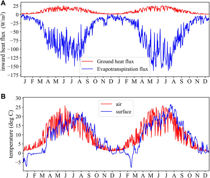
FIGURE 4. Two-year meteorological record of (A) heat flux from solar radiation and evaporation; (B) temperature of air and ground surface.

λ is the latent heat of vaporization. (e_s - e_a) represents the vapor pressure deficit to air, ρ_a is the mean air density under the constant air pressure, C_pa is the specific heat of air, Δ denotes the gradient of the saturated vapor pressure-temperature relationship, γ is the psychrometric constant (γ ≈ 66 Pa/K), r_s is the surface conductance, and r_a is air conductance, which is calculated by the wind speed (v_wind) through r_a = 208/v_wind. Based on Eq. 7 and 2-year meteorological records from one station in North Germany, the latent heat of ET is calculated and shown in Figure 4A. The air and surface temperatures shown in Figure 4B are used to calculate R_n, H, and G₀, respectively.

The entire simulation consists of 2 years. In the first year, the heat pump is turned off, and the circulation pump is running in a small rate of 0.02 l/s. Such a long simulation time is assigned to reach an energy balance condition. Sequentially, the heat pump is turned on and the circulation flow rate $\dot{V}$ is 0.2 l/s. For the parameters of the heat pump, we have used here some assumed typical values. From October to May, the heat pump is in heating mode with a Q_GHE of 5 kW. From June to September, the heat pump is in cooling mode with a Q_GHE of 4 kW. Figure 5 shows the amount of heat extracted or rejected per day, 31 kWh from November to March and 20 kWh from April to October. Usually, the heating and cooling demand is unstable depending on the seasonal climate. The heating or cooling profile can vary greatly from site to site, as the heat or cooling demand of a single house depends on the building material, local climate, as well as its surroundings. Therefore, in this study, we give several ideal assumptions for the hypothetical house. Here we assume that the heat extracted or injected for the house is constant, and the extracted heat will be stored in a storage tank for daily use. The heat demand from several officially reported German data (e.g., local utilities) shows that the daily extracted heat amount we assumed can satisfy part of the heat demand of the house (see Figure A1 in Appendix). That is, we assume that the house can have multiple sources of heating and that the ground source heat pump contributes only partially, probably due to new installation costs. During peak heating seasons, if the heat extracted by the heat pump is not sufficient for the house, other heat sources are used (e.g., gas systems or direct electric heating). On the other hand, since the temperature has continued to rise in Germany in recent years, we assume that in summer, some of the heat from the house will be transferred to the ground. Due to the existence of specific heat pump costs for electricity suppliers in most German states, heat pumps operate continuously on a daily basis during periods of lower electricity prices. These assumptions will apply to all cases similar to the comparison work implemented by Weingaertner (2016), so they should not have an impact on the comparison of the thermal efficiency of variable heat exchangers. It is important to note here that when reaching the daily heat and turning off the heat pump, the value of $\dot{\mathrm{V}}$ is one-10th of the flow rate when the heat pump is on, in order to avoid starting and stopping the circulation pump too often, resulting in additional energy consumption. Throughout the whole year, the heating and cooling modes lasts 242 days and 123 days, respectively. Thus, the ratio heating to cooling days (γ_hc) is 1.97, indicating that this GSHP system is predominantly heating.

FIGURE 5

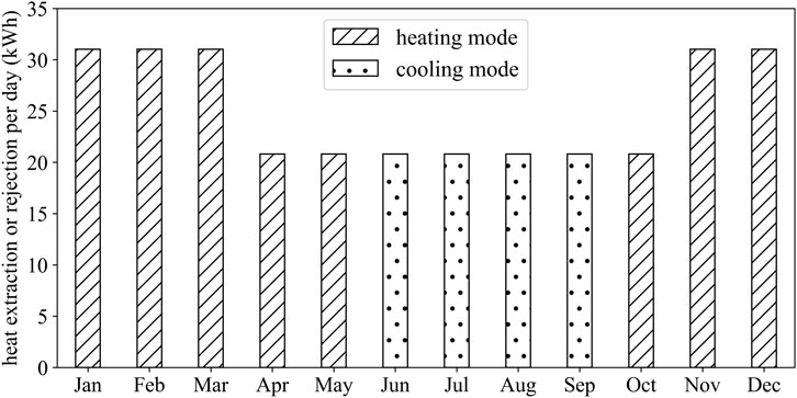
FIGURE 5. Hypothetical daily heat extraction or rejection through the second year.

2.4 Evaluation of 1-year thermal performance

The coefficient of performance of a heat pump (COP_HP) is related to the temperature of the condenser and compressor, the efficiency of the compressor, and the irreversibility of its system. For the simplification, COP_HP can be pre-determined by a quadratic regression equation (Li et al., 2017; Habibi and Hakkaki-Fard, 2018) shown in Eq. 8:

${COP}_{HP}=a\bullet T_{o,f}^2+b{\bullet T}_{o,f}+c(8)$

Eq. 8 indicates that COP_HP can be calculated by the outlet temperature. For the heating mode, a, b, and c are equal to −0.001, 0.133 and 3.257, respectively. For the cooling mode, the values of the three coefficients are −0.003, 0.056 and 5.784. We will use these two equations to approximately calculate COP_HP.

To later compare the temperature of the working fluid, several reference points are defined at certain locations in the pipe (Figure 3, rp1 to rp3). The locations of the three arrangements are identical.

3 Results and discussion

3.1 Comparison of outlet and inlet temperature for three arrangements

The simulated temperatures at the pipe outlet and inlet are shown in Figures 6A, B. In the first year, as the working fluid extracted from the pipe outlet was immediately sent to the outlet without heat extraction, T_o,f and T_i,f were the same as the circulation pump was operating. T_o,f (also T_i,f) were varied from 3.29°C to 11.84°C, 3.00°C–12.18°C, and 2.98°C–12.22°C for the linear-loop, spiral-coil, and slinky-coil arrangements, respectively. The slinky-coil arrangement had the smallest minimum and largest maximum temperature values, as well as the largest temperature difference (linear: 8.55°C, spiral: 9.18°C, slinky: 9.24°C). A comparison of the pipe lengths for the three arrangements shows that the total length of the linear-loop arrangement (66.7 m) is much shorter than the other two arrangements, while the total length of the slinky-coil arrangement is slightly longer than spiral-coil arrangement (239.2 m and 213.2 m). This can be a possible reason why the slinky-coil arrangement has larger temperature fluctuations, since it has larger exchange volume with the environmental influences and heat transfer processes in the soil. In the second year, T_o,f shows the same behavior for the three arrangements. The slinky-coil arrangement still owns the smallest minimum value and largest maximum value. The temperature difference between the maximum and minimum values is generally larger than in the first year due to more heat fluxes and higher surface temperatures during the second year (Figure 4). The difference between the outlet and inlet temperatures (ΔT_f = T_o,f - T_i,f) depends mainly on the Q_GHE and the working fluid properties. Due to the small variations of fluid properties, ΔT_f performed similar as Q_GHE. For example, when Q_GHE is 5 kW (heating mode) then ΔT_f is 5.96°C and when the Q_GHE is 4 kW (cooling mode) then ΔT_f is −4.77°C.

FIGURE 6

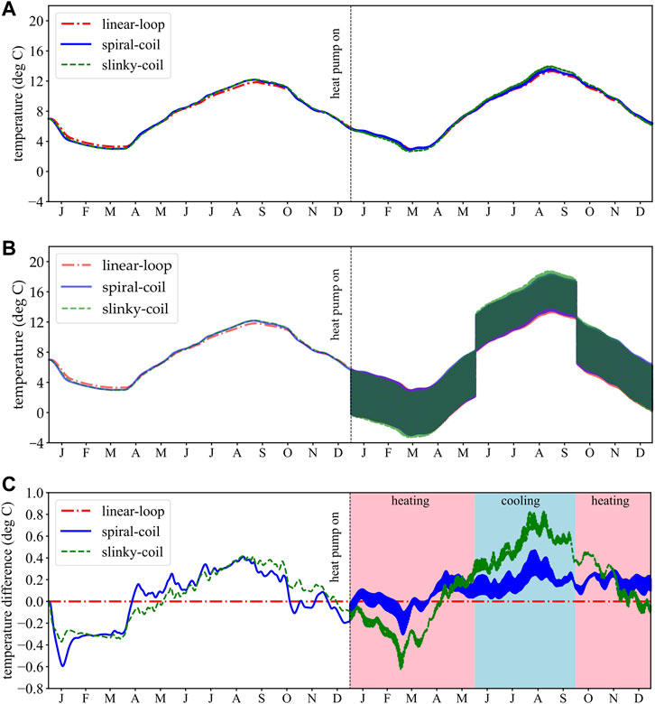
FIGURE 6. Comparison of 2-year temperature evolution at (A) pipe outlet; (B) pipe inlet; (C) temperature difference of pipe outlet between three arrangements (linear-loop arrangement is used as the baseline). The month index indicates the middle of each month.

A detailed comparison between the three arrangements is provided in Figure 6C. The linear-loop arrangement is used as a baseline, and the temperature difference was calculated and shown. Overall, the temperature fluctuations of spiral- and slinky-coil arrangements were stronger than the linear-loop arrangement. In the first year, from January to April, the temperature difference can reach to −0.6°C. From April to November, most of the time, the temperatures were higher than linear-loop arrangement. The maximum temperature difference was around 0.4°C. As the heat pump starts, the temperature fluctuations of the slinky-coil arrangement had larger values. The minimum and maximum changes were about −0.6°C and 0.8°C, respectively.

3.2 Comparison of temperature at different reference points

For a more intuitive comparison, Figure 7 shows the temperature difference between the three reference points and the outlet temperature in the first year. Figure 7A shows that for linear-loop arrangement, from January to the end of July, the temperature at all three reference points is less than the outlet temperature, and the water is heated to a certain extent as it flows through the pipe. rp1 has the lowest temperature, while rp2 has the highest temperature, indicating that the water temperature is heated to the maximum in the middle part of the pipe. In contrast, from August to the end of December, the temperatures at all three reference points are greater than the outlet temperature, indicating that the water is cooled during the process of circulation in the pipe. Again, the cooling effect is best at rp2. However, the spiral- and slinky-coil arrangements exhibit a different trend than the linear one (Figures 7B, C). For both arrangements, the water in the pipe was heated at three reference points from January to about April and from mid-October to December, while it was cooled for the rest of the time. Due to the more three-dimensional shape of spiral coils, the heating and cooling amplitudes were more intense than for slinky coils.

FIGURE 7

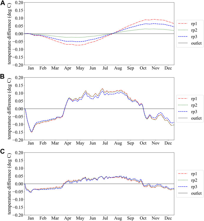
FIGURE 7. Temperature evolution of three arrangement at the first year: (A) linear-loop; (B) spiral-coil; (C) slinky-coil.

For the spiral coils, the heating and cooling effects diminish sequentially from rp1 to rp3, while the opposite is the case for the slinky coils. The temperature change in the second year showed a similar behavior to the first year (Figure 8). A significant difference is that when the heat pump was turned on, the fluid temperature dropped or increased significantly with the heat extracted or discharged daily by the heat pump, as described above.

FIGURE 8

FIGURE 8. Temperature evolution of three arrangement at the second year: (A) linear-loop; (B) spiral-coil; (C) slinky-coil.

3.3 Snapshots of working fluid and ground temperature

Figures 9, 10 illustrate the temperature of the working fluid in the pipe and the ground temperature at z = −1.5 m (bottom of all heat exchangers) at the time of the first heating phase (i.e., t = 365 days) and the first cooling phase (i.e., t = 516 days). The temperature behavior at the beginning of the second heating phase (i.e., t = 638 days) was similar to the temperature behavior at the beginning of the first heating phase and, therefore, is not shown here.

FIGURE 9

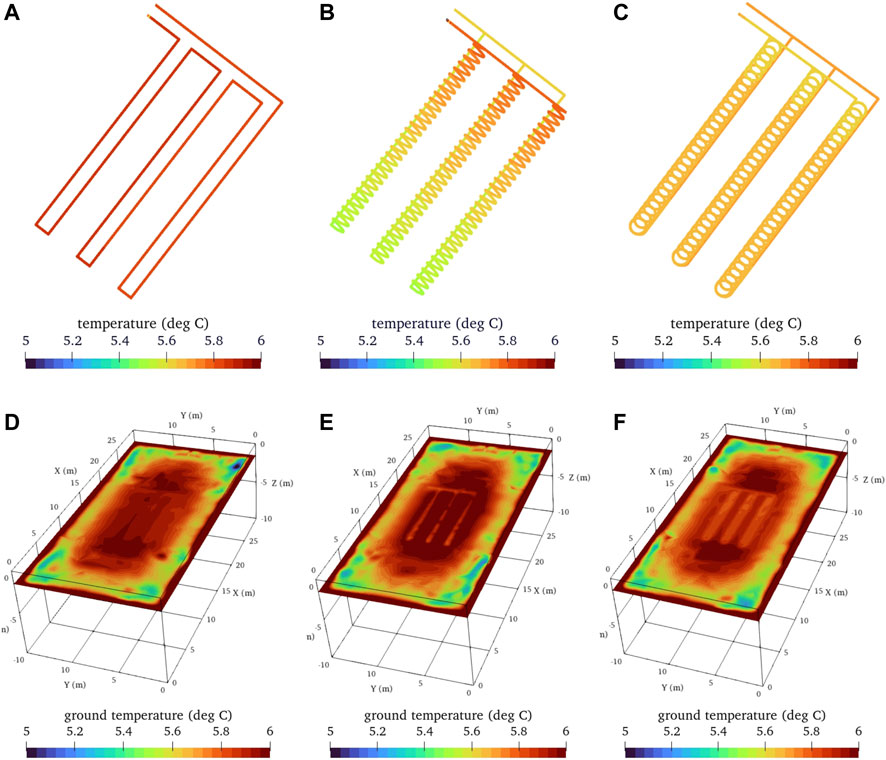
FIGURE 9. Temperature of working fluid in the pipes (A–C) and the ground (D–F) at t = 365 d (A) and (D) linear-loop; (B) and (E) spiral-coil; (C) and (F) slinky-coil.

FIGURE 10

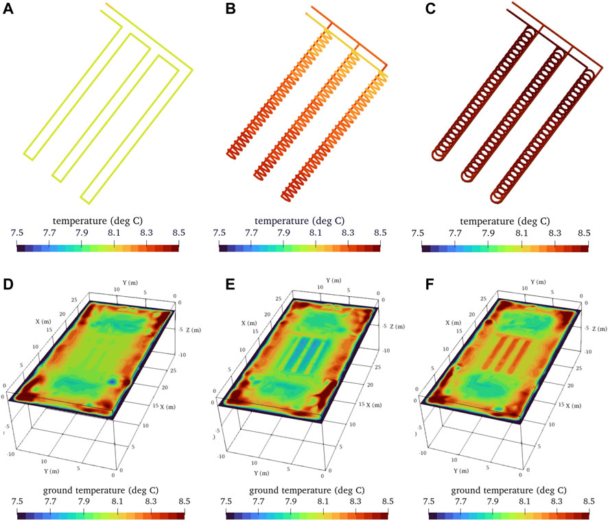
FIGURE 10. Temperature of working fluid in the pipes (A–C) and the ground (D–F) at t = 516 d (A) and (D) linear-loop; (B) and (E) spiral-coil; (C) and (F) slinky-coil.

Figure 9 displays the simulation results at the beginning of the first heating phase (i.e., t = 365 days). After the heat pump extracted the heat from the water at the pipe outlet, the circulating water was reinjected to the inlet, and it was warmed up immediately for all three cases (Figures 9A–C). The fluid lost the heat to the surrounding ground as it flowed in the pipes, indicated by Figures 9D–F. The temperature in the linear loop and spiral heat coils was about 0.15°C higher than in the slinky coils. It is worth noting that for linear and helical coils, although the fluid was heated soon after injection, it was cooled during the flow to the outlet. Conversely, for the slinky coils, the fluid got heated during the circulation in the pipe. This may be due to the shape of the heat exchanger and the mutual interaction between the coils. Slinky coils are stacked more tightly and therefore may lose less heat to the soil. Figures 9D–F show that the temperature of the linear-loop arrangement was slightly lower at the bottom of the exchanger than in the other two cases. As mentioned above, this may be due to the fact that the length and volume of the linear loop are much smaller than the other two arrangements, and therefore the ground temperature distribution from the energy balance simulation presents a more pronounced difference from the other two arrangements.

Figure 10 shows the simulation results at the beginning of the first cooling phase (i.e., t = 516 days). After the heat pump delivered the heat to the water at the pipe outlet, the circulating water was reinjected to the inlet, and it was cooled down immediately for all three cases (Figures 10A–C). The fluid gained the heat from the surrounding ground as it flowed in the pipes, indicated by Figures 10D–F. The fluid temperature in the linear loop and spiral heat coils was about 0.2°C lower than in the slinky coils. Contrary to the beginning of the heating phase, in the case of the linear-loop and spiral-coil arrangements, the fluid was heated during the circulation compared to the temperature at which it was cooled near the inlet of the pipe. And in the slinky coils, their geometry caused that the fluid inside the pipe to be cooled during the circulation.

3.4 Coefficient of performance of heat pump (COP_HP) and economic analysis

COP_HP is merely correlated to the outlet temperature T_o,f, and the temporal changes of COP_HP should be consistent with the fluctuations of T_o,f. Thus, its value throughout the second year is presented statistically as violin plots in Figure 11. A violin plot is a combination of histogram and box plot based on kernel density estimation (Hintze and Nelson, 1998). Table 2 lists a detailed comparison between the three arrangements. In the heating mode, the arithmetic mean of all three arrangements are greater than 4, showing similar magnitudes. The highest value comes from the spiral-coil arrangement. In the cooling mode, the arithmetic mean of all three arrangements are greater than 6, with the highest value coming from the linear-loop arrangement. It is noteworthy that the variance of COP_HP is the smallest in the linear loop case, which indicates better overall performance of this arrangement. Whereas the slinky-coil arrangement shows the least thermal performance in terms of mean and variance of COP_HP. The seasonal performance factor (SPF) was also calculated and shown in the table. The results indicate that the linear-loop arrangement performs best in both heating and cooling modes.

FIGURE 11

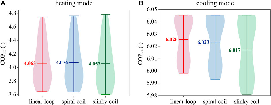
FIGURE 11. Comparison of COP_HP. (A) heating mode; (B) cooling mode).

TABLE 2

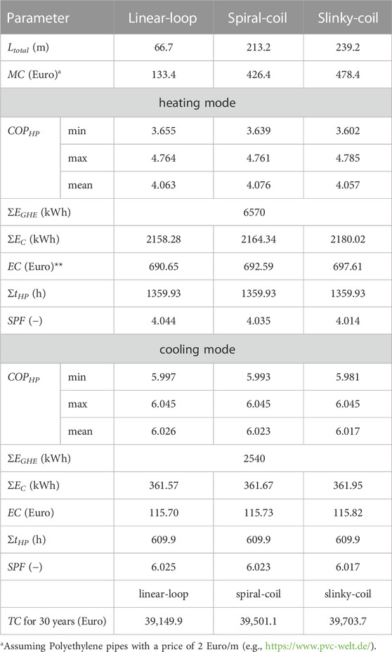
TABLE 2. Comparison of three arrangements.

Although material and installation costs are subject to strong market uncertainties, however, here we mainly compare the price differences between the three arrangements. We therefore assume that the material (outdoor connection and indoor piping and connection) and installation costs are the same for all three arrangements. The total cost of operating the system for 30 years depends primarily on the material cost (MC) of the heat exchanger and the electricity to run the heat pump. The simulation is for 1 year, so the market and interest rate fluctuations are considered small to be neglected. As the shortest length of the linear-loop arrangement, it has the lowest MC, which is around a quarter of the MC of the other two arrangements. Considering an average electricity price of about 0.32 euros/kWh for residential buildings in Germany in 2022 (Eurostat, 2022), for the 1-year heating mode, the total cost of electricity to drive the heat pump compressor (EC) is 690.7, 692.6, and 697.6 Euros, for the linear-loop, spiral-coil, and slinky-coil, respectively. The costs for the cooling mode are even more similar, all around 116 Euros. The total cost (TC) is the sum of the initial MC and the 30-year EC. This comparison demonstrates that the linear-loop arrangement is the most cost-effective. For all the three arrangements, increasing the flow rate increases the rate of heat extraction. Therefore, if the amount of heat extracted or rejected per day is fixed, the operating time will be reduced, thus reducing the cost of electricity for the heat pump. However, the operating cost of the circulation pump will increase due to the increase in the circulation flow rate.

4 Conclusion and outlook

This paper uses numerical models considering the energy balance processes to investigate the thermal and economic performance of three horizontal heat exchanger arrangements. These heat exchangers were used to heat and cool a house for a period of 1 year. The results show that, under the conditions given in this paper, the COP values of the heat pump and the installation and operating costs of the three heat exchangers are similar. Furthermore, the thermal and economic efficiency of the linear heat exchanger has the highest performance when considering the assumptions given in this paper. From this study, we can draw the following conclusions.

• Fully coupled calculations considering energy balances and complex duct geometries can be time-consuming and require powerful computational capabilities. Among the three arrangements, the linear loop arrangement has the shortest simulation time.

• Each arrangement requires proper design, not only for one unit but also for the way multiple units are connected. For the spiral and sliding arrangements, the interaction between the coils needs to be considered. Sensitivity analysis should be performed for different pipe geometries, especially the spacing between coils versus the size of the coils.

• Compared to linear exchangers, both spiral coils, because of their more complex shape, are likely to be more sensitive to environmental factors and the way heat and circulation pumps operate, and thus may have more room for optimization.

In future studies, more complex environmental effects, and hydrothermal processes, such as meteorological data, regional groundwater flow and boundary conditions, conversion between fluid, gas, and solid phases, etc., will be incorporated into the model. Lifetime simulations (e.g., 30–50 years) are necessary to assess the thermal and economic performance and to evaluate the long-term impact of heat pumps and heat exchange systems on the local and regional environment and ecology.

Data availability statement

The original contributions presented in the study are included in the article/Supplementary material, further inquiries can be directed to the corresponding author.

Author contributions

LH: conceptualization, methodology, software, formal analysis, writing-original draft, data curation, visualization. ZR: conceptualization, methodology, software, writing review and editing. LT: writing review and editing. FW: project administration, funding acquisition. All authors contributed to the article and approved the submitted version.

Acknowledgments

We would like to thank the three reviewers for their comments which have improved the quality of our article. We acknowledge financial support by DFG within the funding program Open Access Publikationskosten. LH also acknowledges the research support of Institute of Geosciences at Kiel University.

Conflict of interest

LH and ZR are employed by GeoAnalysis Engineering GmbH.

The remaining authors declare that the research was conducted in the absence of any commercial or financial relationships that could be construed as a potential conflict of interest.

Publisher’s note

All claims expressed in this article are solely those of the authors and do not necessarily represent those of their affiliated organizations, or those of the publisher, the editors and the reviewers. Any product that may be evaluated in this article, or claim that may be made by its manufacturer, is not guaranteed or endorsed by the publisher.

References

Ahmad, S., Rizvi, Z. H., Arp, J. C. C., Wuttke, F., Tirth, V., and Islam, S. (2021). Evolution of temperature field around underground power cable for static and cyclic heating. Energies (Basel) 14, 8191. doi:10.3390/en14238191

CrossRef Full Text | Google Scholar

Al-Ameen, Y., Ianakiev, A., and Evans, R. (2018). Recycling construction and industrial landfill waste material for backfill in horizontal ground heat exchanger systems. Energy 151, 556–568. doi:10.1016/j.energy.2018.03.095

CrossRef Full Text | Google Scholar

Aydın, M., Sisman, A., Gultekin, A., and Dehghan, B. (2015). “An experimental performance comparison between different shallow ground heat exchangers,” in World Geothermal Conference, Melbourne, Australia, 19-25 April, 2015 (IEEE).

Google Scholar

Bottarelli, M., Bortoloni, M., and Su, Y. (2015). Heat transfer analysis of underground thermal energy storage in shallow trenches filled with encapsulated phase change materials. Appl. Therm. Eng. 90, 1044–1051. doi:10.1016/j.applthermaleng.2015.04.002

CrossRef Full Text | Google Scholar

Cao, S. J., Kong, X. R., Deng, Y., Zhang, W., Yang, L., and Ye, Z. P. (2017). Investigation on thermal performance of steel heat exchanger for ground source heat pump systems using full-scale experiments and numerical simulations. Appl. Therm. Eng. 115, 91–98. doi:10.1016/j.applthermaleng.2016.12.098

CrossRef Full Text | Google Scholar

Casasso, A., and Sethi, R. (2014). Efficiency of closed loop geothermal heat pumps: a sensitivity analysis. Renew. Energy 62, 737–746. doi:10.1016/j.renene.2013.08.019

CrossRef Full Text | Google Scholar

Congedo, P. M., Colangelo, G., and Starace, G. (2012). CFD simulations of horizontal ground heat exchangers: a comparison among different configurations. Appl. Therm. Eng. 33–34, 24–32. doi:10.1016/j.applthermaleng.2011.09.005

PubMed Abstract | CrossRef Full Text | Google Scholar

Cuadra, S. V., Kimball, B. A., Boote, K. J., Suyker, A. E., and Pickering, N. (2021). Energy balance in the DSSAT-CSM-CROPGRO model. Agric Meteorol 297, 108241. doi:10.1016/j.agrformet.2020.108241

CrossRef Full Text | Google Scholar

Dasare, R. R., and Saha, S. K. (2015). Numerical study of horizontal ground heat exchanger for high energy demand applications. Appl. Therm. Eng. 85, 252–263. doi:10.1016/j.applthermaleng.2015.04.014

CrossRef Full Text | Google Scholar

Gan, G. (2013). Dynamic thermal modelling of horizontal ground-source heat pumps. Int. J. Low-Carbon Technol. 8, 95–105. doi:10.1093/ijlct/ctt012

CrossRef Full Text | Google Scholar

Gan, G. (2018). Dynamic thermal performance of horizontal ground source heat pumps – the impact of coupled heat and moisture transfer. Energy 152, 877–887. doi:10.1016/j.energy.2018.04.008

CrossRef Full Text | Google Scholar

Go, G. H., Lee, S. R., Yoon, S., and Kim, M. J. (2016). Optimum design of horizontal ground-coupled heat pump systems using spiral-coil-loop heat exchangers. Appl. Energy 162, 330–345. doi:10.1016/j.apenergy.2015.10.113

CrossRef Full Text | Google Scholar

Habibi, M., and Hakkaki-Fard, A. (2018). Evaluation and improvement of the thermal performance of different types of horizontal ground heat exchangers based on techno-economic analysis. Energy Convers. Manag. 171, 1177–1192. doi:10.1016/j.enconman.2018.06.070

CrossRef Full Text | Google Scholar

Hintze, J. L., and Nelson, R. D. (1998). Violin plots: a box plot-density trace synergism. Am. Statistician 52, 181–184. doi:10.1080/00031305.1998.10480559

CrossRef Full Text | Google Scholar

Hou, G., Taherian, H., Song, Y., Jiang, W., and Chen, D. (2022). A systematic review on optimal analysis of horizontal heat exchangers in ground source heat pump systems. Renew. Sustain. Energy Rev. 154, 111830. doi:10.1016/j.rser.2021.111830

CrossRef Full Text | Google Scholar

Kim, M. J., Lee, S. R., Yoon, S., and Go, G. H. (2016). Thermal performance evaluation and parametric study of a horizontal ground heat exchanger. Geothermics 60, 134–143. doi:10.1016/j.geothermics.2015.12.009

CrossRef Full Text | Google Scholar

Kupiec, K., Larwa, B., and Gwadera, M. (2015). Heat transfer in horizontal ground heat exchangers. Appl. Therm. Eng. 75, 270–276. doi:10.1016/j.applthermaleng.2014.10.003

CrossRef Full Text | Google Scholar

Li, C., Cleall, P. J., Mao, J., and Muñoz-Criollo, J. J. (2018). Numerical simulation of ground source heat pump systems considering unsaturated soil properties and groundwater flow. Appl. Therm. Eng. 139, 307–316. doi:10.1016/j.applthermaleng.2018.04.142

CrossRef Full Text | Google Scholar

Li, C., Mao, J., Peng, X., Mao, W., Xing, Z., and Wang, B. (2019). Influence of ground surface boundary conditions on horizontal ground source heat pump systems. Appl. Therm. Eng. 152, 160–168. doi:10.1016/j.applthermaleng.2019.02.080

CrossRef Full Text | Google Scholar

Li, C., Mao, J., Zhang, H., Xing, Z., Li, Y., and Zhou, J. (2017). Numerical simulation of horizontal spiral-coil ground source heat pump system: sensitivity analysis and operation characteristics. Appl. Therm. Eng. 110, 424–435. doi:10.1016/j.applthermaleng.2016.08.134

CrossRef Full Text | Google Scholar

Li, H., Nagano, K., and Lai, Y. (2012a). A new model and solutions for a spiral heat exchanger and its experimental validation. Int. J. Heat. Mass Transf. 55, 4404–4414. doi:10.1016/j.ijheatmasstransfer.2012.03.084

CrossRef Full Text | Google Scholar

Li, H., Nagano, K., and Lai, Y. (2012b). Heat transfer of a horizontal spiral heat exchanger under groundwater advection. Int. J. Heat. Mass Transf. 55, 6819–6831. doi:10.1016/j.ijheatmasstransfer.2012.06.089

CrossRef Full Text | Google Scholar

Liu, Y., Huang, G., Lu, J., Yang, X., Zhuang, C., and Qin, J. (2020). A novel 2-D ring-tubes model and numerical investigation of heat and moisture transfer around helix ground heat exchanger. Geothermics 85, 101789. doi:10.1016/j.geothermics.2019.101789

CrossRef Full Text | Google Scholar

Meng, X., Han, Z., Hu, H., Zhang, H., and Li, X. (2021). Studies on the performance of ground source heat pump affected by soil freezing under groundwater seepage. J. Build. Eng. 33, 101632. doi:10.1016/j.jobe.2020.101632

CrossRef Full Text | Google Scholar

Monteith, J. L. (1965). Evaporation and environment. Symp. Soc. Exp. Biol. 19, 205–234.

PubMed Abstract | Google Scholar

Naylor, S., Ellett, K. M., and Gustin, A. R. (2015). Spatiotemporal variability of ground thermal properties in glacial sediments and implications for horizontal ground heat exchanger design. Renew. Energy 81, 21–30. doi:10.1016/j.renene.2015.03.006

CrossRef Full Text | Google Scholar

Penman, H. L. (1948). Natural evaporation from open water, hare soil and grass. Proc. R. Soc. Lond A Math. Phys. Sci. 193, 120–145. doi:10.1098/rspa.1948.0037

PubMed Abstract | CrossRef Full Text | Google Scholar

Pereira, L. S., Allen, R. G., Smith, M., and Raes, D. (2015). Crop evapotranspiration estimation with FAO56: past and future. Agric. Water Manag. 147, 4–20. doi:10.1016/j.agwat.2014.07.031

CrossRef Full Text | Google Scholar

Robinson, D. A., Campbell, C. S., Hopmans, J. W., Hornbuckle, B. K., Jones, S. B., Knight, R., et al. (2008). Soil moisture measurement for ecological and hydrological watershed-scale observatories: a review. Vadose Zone J. 7, 358–389. doi:10.2136/vzj2007.0143

CrossRef Full Text | Google Scholar

Rybach, L. (2022). Global status, development and prospects of shallow and deep geothermal energy. Int. J. Terr. Heat Flow Appl. 5, 20–25. doi:10.31214/ijthfa.v5i1.79

CrossRef Full Text | Google Scholar

Sangi, R., and Müller, D. (2018). Dynamic modelling and simulation of a slinky-coil horizontal ground heat exchanger using Modelica. J. Build. Eng. 16, 159–168. doi:10.1016/j.jobe.2018.01.005

CrossRef Full Text | Google Scholar

Selamat, S., Miyara, A., and Kariya, K. (2016). Numerical study of horizontal ground heat exchangers for design optimization. Renew. Energy 95, 561–573. doi:10.1016/j.renene.2016.04.042

CrossRef Full Text | Google Scholar

Shang, Y., Dong, M., Mu, L., Liu, X., Huang, X., and Li, S. (2019). “The analysis of the evaporation effect on moisture soil under intermittent operation of ground-source heat pump,” in Energy procedia (Netherlands: Elsevier Ltd), 1508–1513. doi:10.1016/j.egypro.2019.01.359

CrossRef Full Text | Google Scholar

Shi, Y., Cui, Q., Song, X., Xu, F., and Song, G. (2022a). Study on thermal performances of a horizontal ground heat exchanger geothermal system with different configurations and arrangements. Renew. Energy 193, 448–463. doi:10.1016/J.RENENE.2022.05.024

CrossRef Full Text | Google Scholar

Shi, Y., Xu, F., Li, X., Lei, Z., Cui, Q., and Zhang, Y. (2022b). Comparison of influence factors on horizontal ground heat exchanger performance through numerical simulation and gray correlation analysis. Appl. Therm. Eng. 213, 118756. doi:10.1016/J.APPLTHERMALENG.2022.118756

CrossRef Full Text | Google Scholar

Sofyan, S. E., Hu, E., and Kotousov, A. (2016). A new approach to modelling of a horizontal geo-heat exchanger with an internal source term. Appl. Energy 164, 963–971. doi:10.1016/j.apenergy.2015.07.034

CrossRef Full Text | Google Scholar

Tang, F., and Nowamooz, H. (2019). Factors influencing the performance of shallow borehole heat exchanger. Energy Convers. Manag. 181, 571–583. doi:10.1016/j.enconman.2018.12.044

CrossRef Full Text | Google Scholar

Weingaertner, A. (2016). Design a geothermal heat pump‘s heat recovery system. COMSOL Blog Available at: https://www.comsol.de/blogs/app-design-a-geothermal-heat-pumps-heat-recovery-system/ (Accessed March 14, 2016).

Google Scholar

Yoon, S., Lee, S. R., and Go, G. H. (2015). Evaluation of thermal efficiency in different types of horizontal ground heat exchangers. Energy Build. 105, 100–105. doi:10.1016/j.enbuild.2015.07.054

CrossRef Full Text | Google Scholar

Zhang, H., Han, Z., Li, G., Ji, M., Cheng, X., Li, X., et al. (2021). Study on the influence of pipe spacing on the annual performance of ground source heat pumps considering the factors of heat and moisture transfer, seepage and freezing. Renew. Energy 163, 262–275. doi:10.1016/j.renene.2020.08.149

CrossRef Full Text | Google Scholar

Zhou, K., Mao, J., Li, Y., Zhang, H., Chen, S., and Chen, F. (2022). Thermal and economic performance of horizontal ground source heat pump systems with different flowrate control methods. J. Build. Eng. 53, 104554. doi:10.1016/j.jobe.2022.104554

CrossRef Full Text | Google Scholar

Zou, H., Pei, P., Wang, C., and Hao, D. (2021). A numerical study on heat transfer performances of horizontal ground heat exchangers in ground-source heat pumps. PLoS One 16, e0250583. doi:10.1371/journal.pone.0250583

PubMed Abstract | CrossRef Full Text | Google Scholar

Appendix

FIGURE A1

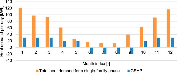
FIGURE A1. Year-round heating demand for a typical single-family house and assumed heating and cooling demand for the model in this study (Source: Stadtwerk München).