Calculation and optimization of inter-regional available transfer capability considering wind power uncertainty and system improvement measures

The intermittency and uncertainty of wind energy make transmission congestion management increasingly complex. In this paper, we investigate the impact of wind energy on available transmission capacity (ATC) and then explore ways to mitigate transmission congestion from the grid and load side, respectively. The impact of a stochastic variable is considered by applying Latin Hypercube Sampling (LHS) and backward curtailment techniques to generate typical scenarios. ATC is improved by the optimal allocation of Thyristor Controlled Series Compensation (TCSC) on the grid side and the use of Demand Response (DR) on the load side. The source-grid-load cooperative optimisation model for ATC is solved by an improved particle swarm optimisation (PSO) algorithm. Based on the IEEE-30 bus system, an experimental scheme is designed and analytical calculations are performed. The results show that the joint application of TCSC and DR can help to improve ATC in a comprehensive way. The work done in this paper can achieve the purpose of promoting renewable energy consumption by improving the utilisation efficiency of the transmission network without changing the network structure.

1 Introduction

1.1 Research motivation

The intermittency and uncertainty of wind power make system operation complex and variable. This tends to cause problems such as the overloading of the transmission line. Available transmission capacity (ATC) is an important parameter that measures the ability of power systems to transmit power between regions (Jiang et al., 2022; Shinde et al., 2023). With the increasing penetration of new energy sources, the application of various new load types, and the high proportion of power electronics in power equipment, it is essential to quantitatively study the impact of wind power uncertainty on ATC and to explore solutions to transmission congestion from the load side and the network side.

1.2 Literature review

Most of the existing studies on ATC, whether using deterministic or probabilistic analysis, are based on the optimal allocation of the source-side resource increase when the load demand increases, or on the optimal dispatch of the grid-connected capacity and the output of conventional units when new energy sources are connected to the grid. For example, Chauhan et al. (2023) presents a novel approach called the modified repeated alternating current power flow with step-size control mechanism to analyze the ATC of the power system during bilateral wheeling transactions. This method saves computation time and is more suitable for ATC calculations of large power systems compared with the conventional methods. Majumdar et al. (2021) constructs an ATC calculation model using the sum of the load node active power increments as the objective function and the static safety and stability of the system as the constraints. The model was solved based on various intelligent optimization algorithms. Sun et al. (2020) proposed an ATC calculation method based on linearized optimal power flow, and experimentally verified that this method is superior to the ATC calculation methods based on DC power flow and AC power flow. Zhang et al. (2020) provided an overview of issues related to the calculation of probabilistic available transmission capacity. Reyad et al. (2023) proposed an approach for ATC assessment in an intraday market. The presented methodology allows the transmission system operator to assess the ATC close to reality, taking into account the voltage stability concerns as well as the uncertainties of the forecasted load and wind power. Wang et al. (2021) solves the probabilistic ATC problem for power systems containing wind farms with the help of opportunity constrained planning.

Whether a system has sufficient ATC is not only related to the optimal dispatch of the active power of the source-side generators, but is also closely related to the load distribution. In the case of a peak load, transmission is often blocked. However, if the load distribution can be adjusted to ensure that the total amount of transmission during a given period is constant with a reduction in the spike, then it would be possible to reduce the occurrence of transmission blockages during that period. Demand response (DR) is a way for customers to adjust their electricity consumption plans in response to market changes based on market price signals or incentives. Some previous studies have been conducted on DR and its application to solve transmission blockage problems. For example, the impact of DR on the ATC of power systems with wind power has been quantified by constructing virtual power plants (Chen et al., 2019a). Wu et al. (2019) solved the transmission blockage problem based on a stochastic chance constraint approach that considers wind power and DR uncertainties. Chen et al. (2019b) proposed a two-stage ATC evaluation framework that combines flexible DR and verifies that flexible DR can effectively improve real-time ATC through load transfer and peak shaving.

With the same generator output configuration and load distribution, the ATC will be different if the network structure is changed. An appropriate network structure can help to improve the ATC, but often a huge investment is required to improve the network structure by adjusting the lines. The flexible AC transmission system (FACTS) combines power electronics technology with traditional power system components (Ahmad et al., 2000). The impact of FACTS on ATC has been explored in some reports. For example, a FACTS optimal allocation method based on the brain storm optimization algorithm has been proposed to improve the ATC (Adewolu and Saha, 2022). Singh et al. (2022) introduced a Lion Updated Moth Flame Optimization algorithm to optimally configure thyristor-controlled series compensation (TCSC) to increase ATC. Moreover, Shen et al. (2000) introduced a unit capacity control scaling factor for the unified power flow controller to quantify its control effect, and, based on this, a method for locating and sizing a unified power flow controller to improve the ATC was proposed.

1.3 Contribution and organization of this paper

To date, few studies have been conducted to improve ATC by combining load-side and network-side measures based on new energy output uncertainty. This paper aims to introduce load-side price-based DR and grid-side TCSC measures to improve ATC based on the study of wind power volatility and uncertainty, compare these measures using a test system, and provide recommendations.

The main contributions are: 1) A method for obtaining typical wind power scenarios is derived; a method for handling load DR is derived; a model for TCSC in steady-state power system calculations is derived. 2) A model for ATC calculation considering wind power uncertainty, load DR, and TCSC is developed. 3) The particle swarm optimization (PSO) algorithm is improved and the solution process is designed. 4) An experimental scheme is set up based on the arithmetic example to validate the theory in the paper.

The remaining chapters are organized as follows: Section 2 introduces the treatment of wind power stochasticity, the principle of load-demand response, and the model of TCSC in steady-state calculation. Section 3 introduces the model of source-network-load cooperative optimization of inter-area ATC. Section 4 focuses on the improvement of the PSO algorithm and the design of the solution process for the model developed in the paper. Section 5 focuses on the design of an experimental scheme based on the arithmetic example to validate the related theory and model. Section 6 presents the conclusion.

2 Wind power uncertainty treatment method, load DR principle, and TCSC equivalent model

2.1 Wind power uncertainty treatment method

Wind turbine output is stochastic and there may be deviations between actual and predicted output. The predicted deviation of the average wind turbine output follows a normal distribution (Yang et al., 2022). Importantly, if the deviation set is generated with specific tools based on the probability distribution of the predicted deviation, then a small number of typical representative scenarios can be obtained by reducing the original scenarios to reflect the distribution of the original scenarios. Thus, the wind turbine output is transformed from a random problem to a deterministic problem. In this paper, the initial set of deviation scenarios was generated using Latin hypercube sampling (Avila and Chu, 2019), and the typical representative error scenarios and their corresponding probabilities were obtained using the backward reduction technique (Wei et al., 2000). The set of actual typical wind turbine output scenarios was obtained by adding the typical deviation scenarios to the predicted wind turbine output curve, as given by Eq. 1.

$P_{\mathrm{w},t}^{\mathrm{s}}=P_{\mathrm{w},t}^{\mathrm{y}}+\Delta P_{\mathrm{w},t}(1)$

where P^s_w,t and P^y_w,t are the actual and predicted outputs of the turbine at time t, respectively, and ΔP_w,t is the predicted error of the turbine output at time t.

The specific implementation steps of the Latin hypercube sampling were as follows: first, the sampling size was set to M; then the value space (0, 1) of the probability distribution function Y was equally divided into M parts {i.e., (0, 1/M), [(M-1)/M, 1]}; next, one point from each interval, Ya, was randomly selected; and finally, the inverse function Eq. 2 was used to obtain the sampling point x_a to form the initial scenario set.

$x_a=F^{-1}\left({\mathrm{Y}}_a\right)a=1,\cdots ,M(2)$

The specific implementation steps of the backward reduction technique were as follows:

1) The initial probability of each scenario in the original scenario set was set to 1/M.

2) The probability distance between scenario x_a and the other scenarios was calculated. The minimum probability distance D_a and the scenario x_b, corresponding to this minimum value, were recorded. D_a was calculated using Eq. 3.

$D_a=\min \left({\lambda }_{a}d\left(x_a,x_b\right)\right)a,b=1,\cdots ,M\mathrm{a}\mathrm{n}\mathrm{d}a\ne b(3)$

where λ_a is the probability of scenario x_a and d(x_a, x_b) is the Euclidean distance between scenarios x_a and x_b.

3) The minimum value of D_a and its corresponding scenario x_a, which is the scenario to be deleted, was determined. The minimum value of D_a was named D_min, as shown in Eq. 4.

$D_{\min }=\min \left(D_a\right)a=1,\cdots ,M(4)$

4) The scenario x_a selected in step 3 was eliminated and its probability was superimposed on the probability of the sample x_b determined in step 2 to ensure that the sum of the probabilities of the sample remained constant at 1.

5) The total number of samples M was decreased by 1, and it was judged whether the reduction requirement was met; if not, steps 2–4 were repeated until the remaining number of scenarios met the requirement.

2.2 Load DR principle

Load-side management uses price-based DR (Zhao et al., 2021). Based on the original load curve and the time-of-use tariff to guide customer’s electricity consumption behavior, the load distribution is changed while ensuring that the total load remains unchanged. From the customer’s perspective, DR minimizes electricity consumption when the price is high and shifts some elastic demand to when the price is low. From the power company’s perspective, DR increases the price to reduce pressure on the power supply when customers are using a lot of electricity and reduces the price to encourage electricity consumption when the load is low. When the DR quantity is obtained for each period, this quantity can be superimposed on the initial load to obtain the load after implementing the DR, as given by Eq. 5.

$L_t^{\mathrm{D}\mathrm{R}}=L_t+\Delta L_t(5)$

where L_t and L^DR_t are the loads before and after DR in period t, respectively, and ΔL_t is the amount of load DR in period t.

The quantity of DR for each period was obtained using the electricity tariff elasticity matrix (Liu et al., 2021), as given by Eq. 6.

$\left[\begin{array}{c}\Delta L_1\\ ⋮\\ \Delta L_t\\ ⋮\\ \Delta L_{\mathrm{T}}\end{array}\right]=\left[\begin{array}{ccccc}{L}_1& \cdots & 0& \cdots & 0\\ ⋮& & ⋮& & ⋮\\ 0& \cdots & L_t& \cdots & 0\\ ⋮& & ⋮& & ⋮\\ 0& \cdots & 0& \cdots & L_{\mathrm{T}}\end{array}\right]\cdot M_{\mathrm{e}}\cdot \left[\begin{array}{c}\Delta C_1/C\\ ⋮\\ \Delta C_t/C\\ ⋮\\ \Delta C_{\mathrm{T}}/C\end{array}\right](6)$

where T is the total number of periods; ΔL_t and L_t denote the load DR quantity and the original load at time t, respectively; M_e is the price elasticity matrix; C is the original fixed electricity price; and ΔC_t is the difference between the time-of-use price and the original fixed price at time t.

The price elasticity matrix M_e represents the relationship between the rate of load change and the rate of price change in each period, as given by Eq. 7.

$M_{\mathrm{e}}=\left[\begin{array}{ccccc}{M}_{11}& \cdots & M_{1m}& \cdots & M_{1\mathrm{T}}\\ ⋮& & ⋮& & ⋮\\ M_{t1}& \cdots & M_{tm}& \cdots & M_{t\mathrm{T}}\\ ⋮& & ⋮& & ⋮\\ M_{\mathrm{T}1}& \cdots & M_{\mathrm{T}m}& \cdots & M_{\mathrm{T}\mathrm{T}}\end{array}\right],{\mathrm{M}}_{ij}=\frac{\Delta L_t/L_t}{\Delta C_m/C}(7)$

where M_tm is the elasticity coefficient (if t is equal to m, it is the coefficient of self-elasticity; if t and m are not equal, it is the coefficient of mutual elasticity). In the calculation, the self-elasticity and mutual elasticity coefficients were approximated by −0.3 and 0, respectively.

2.3 TCSC equivalent model

The TCSC consists of a capacitor and a thyristor-controlled reactor. By adjusting the conduction angle of the thyristor, the reactance of the TCSC can be varied (Siddiqui and Prasgant, 2022). This makes the line equivalent impedance becomes a controllable parameter. Its connection to the system is shown in Figure 1.

FIGURE 1

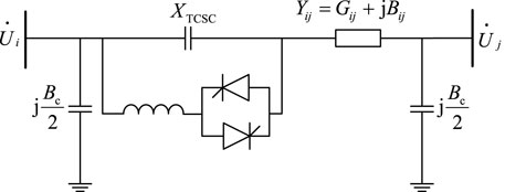
FIGURE 1. The connection between the TCSC and the power system.

The variation process of the line parameters is shown by Eq. 8.

$\left\{\begin{array}{c}{X}_{ij}^{\prime }=X_{ij}+X_{\mathrm{T}\mathrm{C}\mathrm{S}\mathrm{C}}\\ X_{\mathrm{T}\mathrm{C}\mathrm{S}\mathrm{C}}=-{\beta }_{\mathrm{T}\mathrm{C}\mathrm{S}\mathrm{C}}{X}_{ij}\end{array}\right.(8)$

where i and j are the node serial numbers, X_ij and X_ij^′ are the reactance of the line before and after compensation, respectively, and β_TCSC is the compensation degree.

3 Source-grid-load synergy model for optimizing the interregional ATC

The model of the source-grid-load synergistic optimization ATC was constructed by Eq. 9.

$\left\{\begin{array}{c}F\left(\mathbf{x}\right)=\max f\left(\mathbf{x}\right)\\ s.t.\left\{\begin{array}{c}{g}_{\beta }\left(\mathbf{x}\right)\le 0,\beta =\mathrm{1,2},\cdots \\ h_{\gamma }\left(\mathbf{x}\right)=0,\gamma =\mathrm{1,2},\cdots \end{array}\right.\end{array}\right.(9)$

where F(x) is the objective function; x is an α-dimensional control variable (x₁, x₂, … , x_α); and g_β(x) and h_γ(x) are the βth inequality constraint function and the γth equality constraint function, respectively. The corresponding terms are described as follows.

3.1 Objective function

The objective function f(x) is the interregional ATC. As defined by the North American Electric Reliability Council, the ATC is the remaining transmission capacity available for commercial use after the maximum transmission capacity of the transmission section minus contracted power and certain transmission margins, the Transmission Reliability Margin (TRM) and the Capacity Benefit Margin (CBM). Ignoring the TRM and CBM, the ATC was set approximately as the maximum transmission capacity of the transmission section minus the contracted power. That is, while ensuring that generation and load in other regions remained unchanged, the output of generators in the sending area and the load of the receiving area were simultaneously increased until the transmission capacity of line reached the limit. The sum of the increased output of the sending region is the ATC from the sending region to the receiving region (Karuppasamypandiyan et al., 2021), as shown in Eq. 10.

$\mathrm{A}\mathrm{T}\mathrm{C}={\displaystyle \sum _{i\in N_{\mathrm{G}\mathrm{S}}}}\Delta P_{\mathrm{G}i}(10)$

where ∆P_Gi is the increase in the active power of the generator connected to node i in the transmission area relative to its base-state value, and N_GS is the set of nodes with generators in the transmission area.

3.2 Constraint conditions

3.2.1 Equality constraints

The equation constraint h_γ(x) mainly includes the power balance constraint of each node in the system, as given by Eq. 11.

$\left\{\begin{array}{c}\begin{array}{l}\left(P_{\mathrm{G}i}+\Delta P_{\mathrm{G}i}\right)+P_{\mathrm{W}i}^{s,t}-\left(1+{\eta }_i\right)P_{\mathrm{D}i}^{\mathrm{D}\mathrm{R},t}=\\ U_i{\displaystyle \sum _{j=1}^{\mathrm{q}}}{U}_j\left(G_{ij}\cos {\theta }_{ij}+B_{ij}\sin {\theta }_{ij}\right)\end{array}\\ \begin{array}{l}{Q}_{\mathrm{G}i}+Q_{\mathrm{W}i}^{s,t}-\left(1+{\eta }_i\right)Q_{\mathrm{D}i}^{\mathrm{D}\mathrm{R},t}=\\ U_i{\displaystyle \sum _{j=1}^{\mathrm{q}}}{U}_j\left(G_{ij}\sin {\theta }_{ij}-B_{ij}\cos {\theta }_{ij}\right)\end{array}\end{array}\right.(11)$

where P_Gi and Q_Gi are the active and reactive powers of the generator connected to node i, respectively; ∆P_Gi is the active power increase of the unit connected to node i; P^s,t_Wi and Q^s,t_Wi are the active and reactive powers of the wind farm connected to node i at time t under scenario s, respectively; P^DR,t_Di and Q^DR,t_Di are the active and reactive power of the load connected to node i at time t, respectively, after taking DR into account; η_i is the load growth rate; U_i and U_j are the voltage magnitudes of node i and j, respectively; θ_ij is the difference in the phase angle of the voltage between the two nodes; G_ij and B_ij are the corresponding elements in the node admittance matrix; and q is the number of nodes connected to node i. If it is not a transmitting zone, ∆P_Gi is set to 0. If it is not a receiving zone, η_i is set to 0. If the branch is configured with the TCSC, the branch reactance is changed according to Formula 8, and only G_ij and B_ij of the corresponding branch are changed in the power balance relationship equation.

3.2.2 Inequality constraint

The inequality constraint g_β(x) includes the control variable constraint and the state variable constraint.

The control variable constraints mainly include the proportional constraint of the load involved in the DR, the location constraint of the TCSC configuration, the range constraint of the value of the compensation degree, and the active power range constraint of the generator in the supply area, as shown in Eq. 12.

$\left\{\begin{array}{c}\lambda \in \left\{\mathrm{0,0.6}\right\}\\ B\in N_{\mathrm{b}}\\ {\beta }_{\mathrm{T}\mathrm{C}\mathrm{S}\mathrm{C}}^{\min }\le {\beta }_{\mathrm{T}\mathrm{C}\mathrm{S}\mathrm{C}}\le {\beta }_{\mathrm{T}\mathrm{C}\mathrm{S}\mathrm{C}}^{\max }\\ P_{\mathrm{G}i}^{\min }\le P_{\mathrm{G}i}+\Delta P_{\mathrm{G}i}\le P_{\mathrm{G}i}^{\max },i\in N_{\mathrm{G}\mathrm{S}}\end{array}\right.(12)$

where λ is the proportion of the node load involved in the DR (the value is set to 0 or 0.6); B and N_b denote the serial number of the branch configured with the TCSC and the set of all the branch serial numbers in the system, respectively; β^max _TCSC and β^min _TCSC are the upper and lower limits of the TCSC compensation degree, respectively; P_Gi and ∆P_Gi denote the active power of the generator connected to node i in the sending area at the base-state power flow and the increment relative to this value, respectively; and N_GS denotes the set of nodes with generators in the sending area.

The state variable constraints mainly include the voltage magnitude constraint of the load node, the reactive power constraint of the generator, and the branch transmission upper limit constraint, as given by Eq. 13.

$\left\{\begin{array}{c}{U}_i^{\min }\le U_i\le U_i^{\max },i\in N_{\mathrm{D}}\\ {\mathrm{Q}}_j^{\min }\le Q_j\le {\mathrm{Q}}_j^{\max },j\in N_{\mathrm{G}}\\ \left|S_{br}\right|\le S_{br}^{\max },br\in N_{\mathrm{b}}\end{array}\right.(13)$

where U^max _i and U^min _i are the upper and lower limits of the voltage amplitude of load node, respectively; N_D is the set of load nodes; Q^max _j and Q^min _j are the upper and lower limits of the reactive power of generator, respectively; N_G is the set of generator nodes; and S_br and S^max _br are the capacity and its upper limit of the branch br, respectively. N_b has the same meaning as the corresponding parameter in Eq. 12 and represents the set of all branch serial numbers in the system.

3.3 Constraint handling strategy

The control variables can be artificially set and can satisfy the constraints by themselves. Meanwhile, the state variables change with the control variables and cannot satisfy the constraints by themselves. When a state variable crosses the boundaries, the crossed amount is added to the original objective function in the form of a penalty term to construct an objective function that considers the inequality constraint, thus forcing the variables to gradually search for non-inferior solutions in the direction of satisfying the constraints (Li et al., 2000), as shown by Eq. 14.

$f\left(\mathbf{x}\right)=f\left(\mathbf{x}\right)-H\left(\mathbf{x},\mathbf{u}\right)(14)$

where x has the same meaning as the corresponding variable in Eq. 5 and represents the control variable; u is the state variable; and H(x, u) is the penalty term and is calculated as in Eq. 15.

$H\left(\mathbf{x},\mathbf{u}\right)={\displaystyle \sum _{i\in N_{\mathrm{D}}}}\frac{\Delta U_i}{U_i^{\max }-U_i^{\min }}+{\displaystyle \sum _{br\in N_{\mathrm{b}}}}\frac{\Delta S_{br}}{S_{br}^{\max }}(15)$

where U^max_i, U^min_i, and S^max_br are the same as the corresponding variables in Formula 13. The intermediate variables can be calculated using Eq. 16.

$\left\{\begin{array}{c}\Delta U_i=\left\{\begin{array}{c}{U}_i^{\min }-U_i,U_i<U_i^{\min }\\ 0,U_i^{\min }\le U_i\le U_i^{\max }\\ U_i-U_i^{\max },U_i^{\max }<U_i\end{array}\right.\\ \Delta S_{br}=\left\{\begin{array}{c}\left|S_{br}\right|-S_{br}^{\max },\left|S_{br}\right|>S_{br}^{\max }\\ 0,\left|S_{br}\right|\le S_{br}^{\max }\end{array}\right.\end{array}\right.(16)$

4 Improved PSO algorithm and model solving process

The model in this paper is a constrained non-linear optimization problem. The improved PSO algorithm, which was formed by improving the initial particle formation method and the particle update rules in the optimization search process based on the PSO algorithm (Sun et al., 2021), was applied to solve this model.

4.1 Coding and good point set initialization

The control variable x is coded with real numbers [λ, B, β_TCSC, ∆P_G1, ∆P_GNGS], where ∆P_G1, ∆P_GNGS are the increments of the active power of the generators in the transmission range. The more uniformly the initial particle population is distributed in the search space, the better it is for improving the optimization efficiency and solution accuracy of the algorithm. The initial particles of the standard PSO optimization algorithm were generated randomly. This method of initial particle generation does not guarantee that the initial particles are uniformly distributed in the search space. The good point set is useful to improve the uniformity and diversity of the initial population. Therefore, the good point set was used to initialize the population.

The principle of good point set initialization (Yan et al., 2000) and the steps to obtain a good point set were as follows:

1) G_α denotes the unit cube of the α-dimensional Euclidean space. There is a point set P(k) containing n points in G_α. P(k) = {[y₁(k), … , y_d(k), … , y_α(k)]|k = 1, 2, …, n}, where y_d(k) denotes the dth dimension of the kth point.

2) Let each point r in G_α be (r₁, … , r_d, … , r_α). N(r) denotes the number of points satisfying 0≤y_d(k)<r_d in P(k). Let φ(n) = sup|N(r)/n-|r|| and call it the deviation of P(k). If φ(n) = o(1) for any n, then P(k) is said to be a good point set on G_α.

3) In this paper we have adopted the method of dividing the circular domain to construct the good point set. That is, we let the point r=[2cos(2π/p), 2cos(4π/p), …, 2cos(2dπ/p)], where p is the smallest prime number among the numbers not less than 2α+3, and then let the good point set P(k) = {[(r₁k), … , (r_dk), … , (r_αk)]|k = 1, 2, … , n}, where (r_dk) denotes taking the fractional part.

4) Map each point in P(k) to the search space, as shown in Eq. 17.

$x_{k,d}=\left(u{b}_d-l{b}_d\right)·\left\{r_{d}k\right\}+l{b}_d(17)$

where x_k,d denotes the dth dimension of the kth initial particle, and ub_d and lb_d denote the upper and lower bounds of the dth dimension control variables, respectively.

4.2 Variable inertia weighting factor setting

In order to improve the global search speed in the early stage and the local search ability in the later stage, as well as to remove the limitation of having to set the velocity variation range precisely (Zhang et al., 2000), the weighting coefficient was set to decrease linearly with the number of iterations in a given value interval. The rules for updating the particle velocity and position are shown in Eq. 18.

$\left\{\begin{array}{c}{v}_{k,d}^{it+1}=w{v}_{k,d}^{it}+c_1{r}_1\left(p_{k,d}-x_{k,d}^{it}\right)+c_2{r}_2\left(g_d^{it}-x_{k,d}^{it}\right)\\ x_{k,d}^{it+1}=x_{k,d}^{it}+v_{k,d}^{it+1}\\ w=w_{\max }-\left(w_{\max }-w_{\min }\right)\frac{it}{i{t}_{\max }}\end{array}\right.(18)$

where x^it _k,d and v^it _k,d denote the position and velocity of the dth dimensional variable of the kth particle, respectively, in the itth iteration; it_max is the maximum number of iterations; c₁ and c₂ are the individual learning and social learning parameters, respectively, taking the value 2; r₁, r₂ are random numbers in the interval (0, 1); p_k,d denotes the optimal position of the kth particle’s dth dimension in the historical search; g^it _d denotes the population’s optimal position of the dth dimensional variable in the itth iteration; w is the inertia weighting coefficient; and w_max and w_min are the maximum and minimum limits of the inertia weighting coefficient, respectively.

4.3 Solution process for the model

The computational flowchart for solving the model of this paper using the improved PSO algorithm is shown in Figure 2.

FIGURE 2

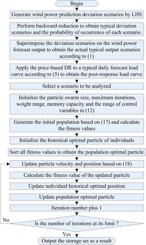
FIGURE 2. Flowchart of model solving based on the improved PSO algorithm.

5 Case study and analysis

5.1 Case and parameter setting

As shown in Figure 3, a wind farm was connected to the system at node 15, based on the IEEE 30-node system. The wind farm contained 20 wind turbines, each with a rated power of 1.5 MW and a stator-side power factor of 1 (Xiao et al., 2000). The ATC from region 3 to region 2 was optimally calculated and the effects of wind power, load DR, and TCSC on the ATC were investigated. The initial number of particles was 20, the storage capacity was 100, the maximum number of iterations was 100, and the inertia weight varied linearly with the number of iterations in the range 0.9–0.4. The base power was 100 MVA, and the power flow was calculated using the Newton–Raphson method.

FIGURE 3

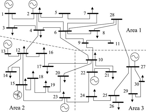
FIGURE 3. Modified IEEE-30 system.

5.2 Wind power related processing and load related processing

The daily load curve, the daily predicted wind turbine output curve, and the time-of-use price curve for a region are shown in Figure 4 (Gao et al., 2000).

FIGURE 4

FIGURE 4. Wind turbine forecast output curve, load curve, and power price curve.

5.2.1 Wind power-related processing

The mean of the normal distribution of the wind power prediction error was taken as 0, and the standard deviation as 0.33% of the rated power. Following the Latin hypercube sampling principle described in Section 2.1, 100 initial scenarios of wind power prediction error were generated to form the initial set of error scenarios, as shown in Figure 5.

FIGURE 5

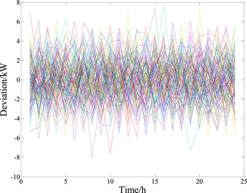
FIGURE 5. Initial deviation scenarios.

Following the principle of the backward reduction technique described in Section 2.1, the initial scenarios in Figure 5 were backward reduced and the number of typical deviation scenarios was set to 10. Furthermore, the typical predicted deviation scenarios of the wind turbine output and their corresponding occurrence probabilities were obtained, as shown in Figure 6.

FIGURE 6

FIGURE 6. Typical deviation scenarios and their respective probabilities.

According to Eq. 1, the predicted wind turbine generator power curve shown in Figure 4 was superimposed on Figure 6 to obtain a typical set of actual wind turbine generator output.

5.2.2 Load-related processing

According to the price-based DR principle described in Section 2.2, for the typical daily load curve shown in Figure 4, 60% of the load was taken to participate in DR. The comparison of the curves before and after DR is shown in Figure 7.

FIGURE 7

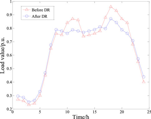
FIGURE 7. Comparison of the load curves before and after the DR.

As shown in Figure 7, the introduction of DR led to a reduction in peak load, with some load being shifted to lower tariff periods, such as late at night. The peak-to-valley difference in the load curve became smaller (0.73 to 0.62 p.u.).

5.3 Simulation and analysis

5.3.1 Hourly ATC optimization calculation

Four schemes were set up for the experimental analysis, as shown in Table 1, where √ indicates that the factor was considered and × indicates that the factor was not considered.

TABLE 1

TABLE 1. Setting of each scheme.

In Scheme 1, the effect of wind power uncertainty on the ATC was investigated. The ATC was calculated for each typical wind power scenario and the ATC curve was plotted. Next, the maximum ATC (ATC_max) and minimum ATC (ATC_min) were determined for each hour to provide the upper and lower bounds for all ATC results. The results are shown in Figure 8.

FIGURE 8

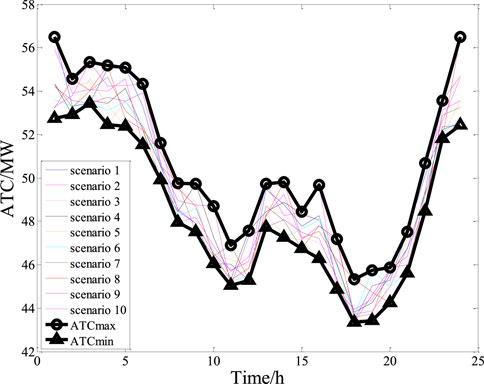
FIGURE 8. ATC under different wind power scenarios (Scheme 1).

As can be seen in Figure 8, the uncertainty in the wind power results in different curves of hourly ATC value for different wind power scenarios. The interval range (i.e., the difference in ATC values) reached a maximum of 4.07 MW (at 24:00) and a minimum of 1.62 MW (at 20:00). The range of ATC_max values was 45.33–56.50 MW and the range of ATC_min values was 43.35–53.50 MW. The ATC curve of each scenario was generally below 56.50 MW, and many ATC values were below 44.50 MW in the 17:00–20:00 time interval.

In addition, the probability of the ATC (ATC_P) for each hour after accounting for wind power uncertainty was tabulated (Table 2).

TABLE 2

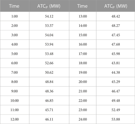
TABLE 2. Hourly ATC_P values considering wind power uncertainty (Scheme 1).

In Scheme 1, the range of values for the hourly ATC_P was 43.81–54.12 MW, with a mean of 49.25 MW, the maximum occurring at 1:00 and the minimum at 18:00 (Table 2). These results correspond to the characteristics of the load curve and the wind turbine output curve shown in Figure 4 for the following reasons: At 1:00, the load demand in zone 2 was lower and the wind farm output was greater; therefore, a large power transfer from zone 3 to zone 2 was avoided, and a higher ATC value was observed at that time. Meanwhile, at 18:00, the load was higher and the wind turbine output was lower. The higher load demand and lower wind energy input in zone 2 meant that a large amount of power had to be transmitted across the zone to meet the load demand. As there was already a large amount of power transfer on the line between zone 3 and zone 2, the ATC value was smaller.

In Scheme 2, the effect of the first improvement measure, the implementation of DR on the load side, was examined. The load curve after DR shown in Figure 7 was used as the load of each node to calculate the ATC for different wind power scenarios. The ATC_max and ATC_min for each hour were determined to form the upper and lower limits of the ATC results for all scenarios, as shown in Figure 9.

FIGURE 9

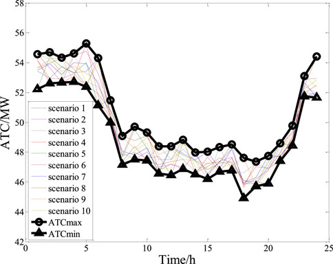
FIGURE 9. ATC considering the load DR (Scheme 2).

In Scheme 2, the ATC_max ranged from 47.36 to 55.28 MW and the ATC_min ranged from 44.92 to 52.72 MW (Figure 9). Compared to Figure 8 (without improvement measures), the ATC curve shown in Figure 9 was generally above 44.50 MW throughout the interval. The apparent improvement of the ATC_min interval indicates that 60% proportional participation of all node loads in DR can improve the ATC, especially the ATC_min.

In addition, the ATC_P values were determined for each hour after the load DR was applied and the results are summarized in Table 3.

TABLE 3

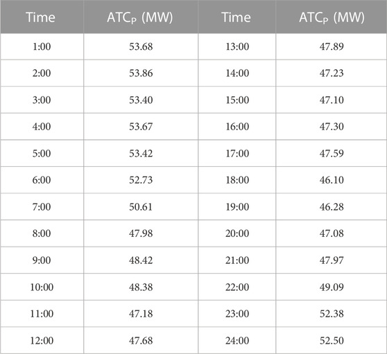
TABLE 3. Hourly ATC_P values considering the load DR (Scheme 2).

In Scheme 2, the ATC_P ranged from 46.10 to 53.86 MW, with a maximum at 2:00 and a minimum at 18:00 (Table 3). The lower limit was higher than the corresponding value without improvement measures (43.81–54.12 MW in Table 2), which confirms the effectiveness of the load DR in improving the ATC_min. The average value of 49.56 MW for the ATC_P was higher than the corresponding value without improvement measures (ATC_P is 49.25 MW in Table 2), thus verifying the improvement of the ATC performance by the DR.

In Scheme 3, the effect of the second improvement measure (i.e., the network-side optimization allocation of the TCSC) was examined. The ATC_max and ATC_min for each hour were determined to form the upper and lower limits of the ATC results for all scenarios, as shown in Figure 10.

FIGURE 10

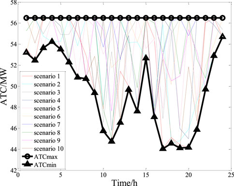
FIGURE 10. ATC considering the TCSC configuration (Scheme 3).

After configuring the TCSC separately for each scenario, the ATC_max reached 56.5 MW (i.e., not limited by the upper limit of the grid transmission, but only by the upper limit of the generator power in the sending area) and the ATC_min ranged from 44.05 to 54.68 MW (Figure 10). Compared to Scheme 1 in Figure 8 (when no improvement measures were taken), many ATC values reached 56.50 MW in several scenarios throughout the time interval shown in Figure 10. This result indicates that a reasonable configuration of the TCSC is effective in improving the ATC, especially the ATC_max.

In addition, the ATC_P was determined for each hour after the optimal allocation of the TCSC, as shown in Table 4.

TABLE 4

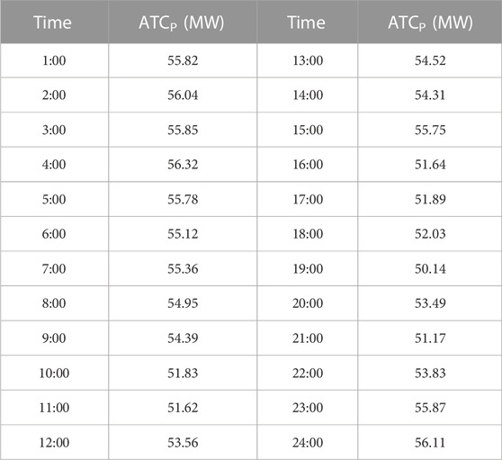
TABLE 4. Hourly ATC_P values considering the TCSC configuration (Scheme 3).

In Scheme 3 (Table 4) the value of the ATC_P ranged from 50.14 to 56.32 MW (in Table 2, the ATC_P was 43.81–54.12 MW). The maximum value of ATC_P occurred at 4:00 and the minimum value occurred at 19:00. The average value of ATC_P was 54.06 MW (ATC_P was 49.25 MW in Table 2). The results shown in Table 4 are much larger than the corresponding values shown in Table 2, which confirms the effectiveness of the optimal configuration of the TCSC for improving ATC.

In Scheme 4, the effect of the combined use of two improvement measures (i.e., optimizing the FACTS configuration and implementing load DR) was examined. The ATC values were calculated for different wind power scenarios, taking into account both the load DR and the optimal configuration of the TCSC. The ATC_max and ATC_min were determined for each hourly ATC to form the upper and lower limits of all of ATC results, as shown in Figure 11.

FIGURE 11

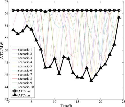
FIGURE 11. ATC considering the load DR and the TCSC configuration (Scheme 4).

When the two improvement measures were combined (Scheme 4), ATC_max reached 56.5 MW and the range of ATC_min was 44.97–55.35 MW (Figure 11). Compared to Scheme 1 (without improvement measures; Figure 8), many ATC values reached 56.50 MW throughout the time interval in Scheme 4 (Figure 11), and the ATC curve was generally greater than 44.5 MW throughout the time interval. This finding indicates that the combined application of the two measures can improve both ATC_max and ATC_min. In terms of improving the ATC_max, the combined application of the two improvement measures (Scheme 4) outperformed the case without any measures (Scheme 1) and the case with only the load DR measure (Scheme 2). Regarding the improvement of ATC_min, the combined application of the two measures (Scheme 4) outperformed the case with no improvement measures (Scheme 1) and the case with the optimally configuring of the TCSC alone (Scheme 3).

In addition, the ATC_P values for each hour after the combination of the two improvement measures were also determined, as shown in Table 5.

TABLE 5

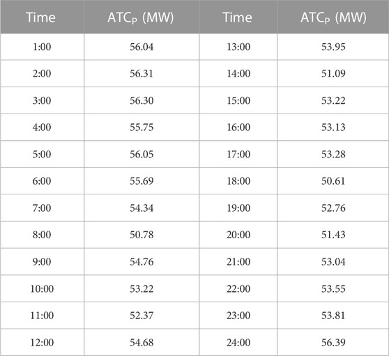
TABLE 5. Hourly ATC_P value considering the load DR and the TCSC configuration (Scheme 4).

In Scheme 4, the range of ATC_P values was 50.61–56.39 MW (this value in Table 2 is 43.81–54.12 MW), with the maximum and minimum values occurring at 24:00 and 18:00 respectively (Table 5). The average value of ATC_P was 53.86 MW (this value in Table 2 is 49.25 MW). The results presented in Table 5 (Scheme 4) are much higher than the corresponding values presented in Table 2 (Scheme 1), thus confirming the effectiveness of the combined application of the two optimization measures in improving the ATC.

5.3.2 Optimizing the ATC with a 24-h cycle

While it was easy to implement DR measures for the load in the case of hourly optimization, the configuration of the TCSC involves the overall adjustment of the TCSC position and the compensation degree during the hourly time interval, which may lead to operational difficulties. To solve this problem, based on the above experiments verifying the effectiveness of the network-side improvement measures, optimization was performed with a whole day as the time period to facilitate the actual operation. The results are shown in Table 6.

TABLE 6

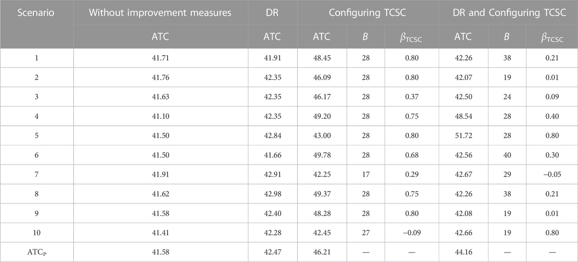
TABLE 6. ATC results and related statistics for a daily optimization cycle.

According to Table 6, the optimized ATC results with load DR measures (column 3) were better than those with no improvement measures (column 2), indicating that DR contributes to improving ATC in all scenarios. The ATC results with the optimal configuration of the TCSC (column 4) were better than those with no improvement measures (column 2), indicating that the configuration of the TCSC helps to improve the ATC for all scenarios. Meanwhile, when implementing DR at the load and optimally configuring the TCSC at the network side (column 7), the ATC results were better than those of the no-improvement-measures scenario (column 2), indicating that measures such as DR and configuring the TCSC contribute to improving the ATC for all scenarios. From the perspective of the ATC_P, the measures with the highest to lowest improvement effects are: optimal allocation of the TCSC (46.21 MW), implementation of load DR and optimal allocation of the TCSC (44.16 MW), and implementation of load DR (42.47 MW). Therefore, after selecting improvement measures according to demand, the relevant equipment locations and compensation parameters can be configured according to columns 5 and 6 or columns 8 and 9.

6 Conclusion

This paper focuses on the calculation and optimization of inter-regional ATC taking into account wind power uncertainties and load-side and grid improvement measures. Modern power systems with increasing penetration of new energy sources place high demands on the transmission capacity of power grids. The traditional method of improving transmission capacity by modifying the network structure has some limitations. In this paper, we explored the methods to improve the transmission capacity of power networks without changing the network structure based on two measures: the optimal configuration of TCSC on the grid side and the implementation of DR on the load side. The proposed random variable processing method, the source-network-load cooperative optimization ATC model, and the improved PSO algorithm for solving the model are of great reference value for solving the problem of transmission congestion in modern power systems. The conclusions drawn from the experiments based on the test system can provide a reference for engineering practice to achieve the purpose of improving the utilization efficiency of the power system and promoting the consumption of new energy. The main findings were as follows.

1) Latin hypercubic sampling and backward curtailment techniques can effectively deal with new energy with stochastic characteristics, thus prompting the transformation of uncertainty problems into deterministic ones. The price-based DR helps to manage loads to change consumption patterns, reduce peak load, narrow peak-to-valley differences, and proactively comply with transmission blockage management. The TCSC can flexibly change the grid structure by adjusting the control parameters, thereby increasing the maximum transmission capacity of the lines.

2) The source-grid-load synergistic optimization model for interregional ATC can quantify the interval of ATC variation due to wind power uncertainty and assess the impact of load-side and network-side improvement measures on ATC.

3) The good point set initialization and the variable inertia weight setting can improve the performance of the PSO algorithm. The improved PSO algorithm can be used to solve constrained non-linear optimization problems.

4) In power systems with new energy sources, load DR effectively improves the lower limit of the ATC interval. The correct configuration of the TCSC is particularly beneficial for improving the upper limit of the ATC interval. The combined application of load DR and optimal allocation of the TCSC contributes to the comprehensive improvement of ATC. From the perspective of the ATC_P of the combined scenarios, the measures with the highest to lowest improvement effects are, in order, the optimal configuration of the TCSC, the load DR, and the optimal configuration of both the TCSC and the load DR.

For the time being, the article does not consider the economic performance of each of the network-side and load-side improvement measures. In the next study, we will add the consideration of economics and re-examine the effect of these two measures on ATC improvement in an integrated manner.

Data availability statement

The original contributions presented in the study are included in the article/Supplementary Material, further inquiries can be directed to the corresponding author.

Author contributions

WL designed the experimental scheme, performed the simulation, analyzed the experimental results, and wrote this paper. TZ participated in the design of the experimental scheme, reviewed the experimental results and this paper. XY reviewed this paper and provided an experimental platform. JW proofread this paper. All authors contributed to the article and approved the submitted version.

Funding

This work was supported by the National Natural Science Foundation of China (Grant Number: 52007103) and the Science and Technology Project of the State Grid (Grant Number: 5211JX1900CX).

Conflict of interest

Author XY was employed by State Grid Jiaxing Power Supply Company.

The remaining authors declare that the research was conducted in the absence of any commercial or financial relationships that could be construed as a potential conflict of interest.

Publisher’s note

All claims expressed in this article are solely those of the authors and do not necessarily represent those of their affiliated organizations, or those of the publisher, the editors and the reviewers. Any product that may be evaluated in this article, or claim that may be made by its manufacturer, is not guaranteed or endorsed by the publisher.

References

Adewolu, B. O., and Saha, A. K. (2022). Optimal setting of thyristor controlled series compensator with brain storm optimization algorithms for available transfer capability enhancement. Int. J. Eng. Res. Afr. 58, 225–246. doi:10.4028/www.scientific.net/jera.58.225

CrossRef Full Text | Google Scholar

Ahmad, A. S., Muhammad, B., Sunusi Sani, A., and Musa, H. (2000). Coordination of multi-type FACTS for available transfer capability enhancement using PI-PSO[J]. IET Generation. Transm. Distribution 14 (21), 4866–4877. doi:10.1049/iet-gtd.2020.0886

CrossRef Full Text | Google Scholar

Avila, N. F., and Chu, C. C. (2019). Distributed probabilistic ATC assessment by optimality conditions decomposition and LHS considering intermittent wind power generation. IEEE Trans. Sustain. Energy 10 (1), 375–385. doi:10.1109/TSTE.2018.2796102

CrossRef Full Text | Google Scholar

Chauhan, Romol, Naresh, R. M. Kenedy, and Aharwar, A. (2023). A streamlined and enhanced iterative method for analysing power system available transfer capability and security. Electr. Power Syst. Res. 223, 109528. doi:10.1016/j.epsr.2023.109528

CrossRef Full Text | Google Scholar

Chen, H., Chu, Y., Zhang, H., Li, L., and Zhang, R. (2019a). Calculation of available transfer capability of wind power grid-connected system considering demand response. J. Northeast Electr. Power Univ. 39 (5), 1–8. doi:10.19718/j.issn.1005-2992.2019-05-0001-08

CrossRef Full Text | Google Scholar

Chen, H., He, X., Jiang, T., and Jiang, Q. (2019b). Integrating flexible demand response toward available transfer capability enhancement. Appl. Energy 251, 113370. doi:10.1016/j.apenergy.2019.113370

CrossRef Full Text | Google Scholar

Gao, H., Zhang, Y., Ji, X., Zhang, X., and Yu, Y. (2000). Scenario clustering based distributionally robust comprehensive optimization of active distribution network. Automation Electr. Power Syst. 44 (21), 32–41. doi:10.7500/AEPS20200307001

CrossRef Full Text | Google Scholar

Jiang, T., Li, X., Kou, X., Zhang, R., Tian, G., and Li, F. (2022). Available transfer capability evaluation in electricity-dominated integrated hybrid energy systems with uncertain wind power: an interval optimization solution. Appl. ENERGY 314, 119001. doi:10.1016/j.apenergy.2022.119001

CrossRef Full Text | Google Scholar

Karuppasamypandiyan, M., Jeyanthy, P. A., Devaraj, D., and Selvi, V. A. I. (2021). Day ahead dynamic available transfer capability evaluation incorporating probabilistic transmission capacity margins in presence of wind generators. Int. Trans. Electr. Energy Syst. 31 (1), e12693. doi:10.1002/2050-7038.12693

CrossRef Full Text | Google Scholar

Li, X., Wang, W., Wang, H., Wu, J., Xu, Q., and Cui, X. (2000). Bi-Level and multi-objective robust optimal dispatching of AC/DC hybrid microgrid with virtual power plant participation. High. Volt. Eng. 46 (7), 2350–2358. doi:10.13336/J.1003-6520.HVE.20200430022

CrossRef Full Text | Google Scholar

Liu, H., Jin, C., and Zhu, X.(2021). An incentive strategy of residential peak-valley price based on price elasticity matrix of demand. Power Syst. Prot. Control 49 (5), 116–123. doi:10.19783/j.cnki.pspc.200527

CrossRef Full Text | Google Scholar

Majumdar, K., Roy, P. K., and Banerjee, S. (2021). Available transfer capability calculation of power systems using opposition selfish herd optimizer. IETE J. Res., 1–15. doi:10.1080/03772063.2021.1960207

CrossRef Full Text | Google Scholar

Reyad, H. W., Elfar, M., and EI-Araby, E. E. (2023). Probabilistic assessment of available transfer capability incorporating load and wind power uncertainties. IEEE Access 11, 39048–39065. doi:10.1109/access.2023.3268544

CrossRef Full Text | Google Scholar

Shen, X. H., Luo, H. M., Gao, W. M., Feng, Y., and Feng, N. (2000). Evaluation of optimal UPFC allocation for improving transmission capacity. Glob. Energy Interconnect. 3 (3), 217–226. doi:10.1016/j.gloei.2020.07.003

CrossRef Full Text | Google Scholar

Shinde, P., Gamberi, G., and Amelin, M. (2023). A multi-agent model for cross-border trading in the continuous intraday electricity market. Energy Rep. 9, 6227–6240. doi:10.1016/j.egyr.2023.05.070

CrossRef Full Text | Google Scholar

Siddiqui, A. S., and Prasgant, (2022). Optimal location and sizing of conglomerate DG-FACTS using an artificial network and heuristic probability distribution mrthodology for modern power system operations. Prot. CONTROL MODEN POWER Syst. 7 (1), 1–25. doi:10.1186/s41601-022-00230-5

CrossRef Full Text | Google Scholar

Singh, J., Yadav, N. K., and Gupta, S. K. (2022). Enhancement of available transfer capability using TCSC with hybridized model: combining lion and moth flame algorithms. Concurrency Comput. Pract Exper 34 (21), e7052. doi:10.1002/cpe.7052

CrossRef Full Text | Google Scholar

Sun, S., Wu, C., Yan, W., Li, M., Liu, Y., and Yang, B. (2021). Optimal power flow calculation method based on random attenuation factor particle swarm optimization. Power Syst. Prot. Control 49 (13), 43–52. doi:10.19783/j.cnki.pspc.201050

CrossRef Full Text | Google Scholar

Sun, X., Rao, Y., Xiao, H., Li, Z., Ruan, C., Teng, W., et al. (2020). Available transfer capability calculation based on linearized optimal power flow[J]. Electr. Power Autom. Equip. 40 (10), 194–199. doi:10.16081/j.epae.202009013

CrossRef Full Text | Google Scholar

Wang, X., Wang, X., Sheng, H., and Lin, X. (2021). A data-driven sparse polynomial chaos expansion method to assess probabilistic total transfer capability for power systems with renewables. IEEE Transaction Power Syst. 36 (3), 2573–2583. doi:10.1109/TPWRS.2020.3034520

CrossRef Full Text | Google Scholar

Wei, B., Han, X., Li, W., Guo, L., and Yu, H. (2000). Multi-time scale stochastic optimal dispatch for AC/DC hybrid microgrid incorporating multi-scenario analysis. High. Volt. Eng. 46 (7), 2359–2369. doi:10.13336/j.1003-6520.hve.20200532

CrossRef Full Text | Google Scholar

Wu, J., Zhang, B., Jiang, Y., Bie, P., and Li, H. (2019). Chance-constrained stochastic congestion management of power systems considering uncertainty of wind power and demand side response. Int. J. Electr. Power & Energy Syst. 107, 703–714. doi:10.1016/j.ijepes.2018.12.026

CrossRef Full Text | Google Scholar

Xiao, Y., Yu, Y., and Zhang, G. (2000). Optimal configuration of distributed power generation based on an improved sooty tern optimization algorithm. Power Syst. Prot. control 50 (3), 148–155. doi:10.19783/j.cnki.pspc.210381

CrossRef Full Text | Google Scholar

Yan, S., Yang, P., Zhu, D., Wu, F., and Yan, Z. (2000). Improved sparrow search algorithm based on good point set. J. Beijing Univ. Aeronautics Astronautics. doi:10.13700/j.bh.1001-5965.2021.0730

CrossRef Full Text | Google Scholar

Yang, N., Qin, T., Wu, L., Huang, Y., Huang, Y., Xing, C., et al. (2022). A multi-agent game based joint planning approach for electricity-gas integrated energy systems considering wind power uncertainty. Electr. Power Syst. Res. 204, 107673. doi:10.1016/j.epsr.2021.107673

CrossRef Full Text | Google Scholar

Zhang, Y., Luo, L., Wang, H., Wang, H., Sheng, G., and Jiang, X. (2000). Method of locating abnormal acoustic source of substation equipment based on MPSO-MLE. High. Volt. Eng. 46 (9), 3145–3153. doi:10.13336/j.1003-6520.hve.20200431

CrossRef Full Text | Google Scholar

Zhang, Y., Zhang, J., He, Y., Yang, Y., and Wang, J. (2020). Review on study for probabilistic available transfer capability in wind farm. Electr. Meas. Instrum. 57 (01), 21–29+54. doi:10.19753/j.issn1001-1390.2020.001.002

CrossRef Full Text | Google Scholar

Zhao, F., Yu, X., Du, S., Guo, C., Xing, H., Fang, Y., et al. (2021). Assessment on flexibility of a power grid with large-scale wind farm integration considering demand response. Power Syst. Prot. Control 49 (1), 42–51. doi:10.19783/j.cnki.pspc.200183

CrossRef Full Text | Google Scholar