A Wasserstein-based distributionally robust neural network for non-intrusive load monitoring

Non-intrusive load monitoring (NILM) is a technique that uses electrical data analysis to disaggregate the total energy consumption of a building or home into the energy consumption of individual appliances. To address the data uncertainty problem in non-intrusive load monitoring, this paper constructs an ambiguity set to improve the robustness of the model based on the distributionally robust optimization (DRO) framework using the Wasserstein metric. Also, for the hard-to-solve semi-infinite programming problem, a novel and computationally efficient upper-layer approximation is used to transform it into an easily solvable regularization problem. Two different data feature extraction methods are used on two open-source datasets, and the experimental results show that the proposed model has good robustness and performs better in identifying devices with large fluctuations. The improvement is about 6% compared to that of the convolutional neural network model without the addition of distributionally robust optimization. The proposed method supports transfer learning and can be added to the neural network in the form of a single-layer net, avoiding unnecessary training times, while ensuring accuracy.

1 Introduction

Most countries around the world are witnessing rapid growth in building energy use; commercial and residential buildings account for more than one-third of the global energy consumption, while accounting for more than 40% of global carbon dioxide emissions (Yoon S H et al., 2018). In order to improve energy efficiency, it is necessary to adopt more suitable energy management techniques (Zhang D et al., 2021) or the use of smart devices to collect more detailed equipment data (Xie H et al., 2023). Since the 1990s, non-intrusive load monitoring (NILM) (Hart G W, 1992) has become one of the dominant frameworks in the field of energy consumption detection (Azizi E et al., 2021; Gillis J M et al., 2017). NILM is a technology that uses electrical data analysis to disaggregate the total energy consumption of a building or home into the energy consumption of individual appliances. This can be achieved without the need for additional hardware sensors, by analyzing the electrical data to identify the energy consumption of each appliance, including energy consumption, frequency of use, and energy peaks. Compared to traditional energy monitoring techniques, NILM technology has the advantages of being non-intrusive, less costly, scalable, and providing more accurate energy consumption data. This technology increases the interaction between electricity suppliers and consumers. For suppliers, NILM can help them understand the power models of various appliances more accurately, and for consumers, they can target specific appliances for a more rational use (Liu Y et al., 2018).

In general, there are two approaches to NILM technology, the event-based approach and the event-less approach. The former method usually performs device identification through state transitions of a single appliance in the total measurement data. The latter often does the matching by separating the sample data of one or more appliances from the aggregated data. In this paper, we adopt an event-based detection method, which has the following steps: event monitoring, feature extraction, and load identification. The task of the event detection phase is mainly to record the changes in aggregated data caused when one or more appliances are activated or when a state transition occurs and then, to extract the features of the data in this phase; the extracted features should maximize the differences between different appliances and minimize the differences between the same appliances (Zheng Z et al., 2018). The selection of an effective set of appliance features is still challenging and an appropriate feature representation can greatly affect the accuracy of appliance recognition (Liu Y et al., 2018), after which the feature can be used in load recognition to identify different appliance classes.

Load recognition is one of the important tasks of NILM, which uses machine learning techniques to extract the electrical feature vectors of each appliance from the aggregate measurements and match them to their respective classes at the output (Azizi E et al., 2021). The electrical appliance feature data are extracted at different sampling rates (high or low frequency) and which data are used depend on the appliance features required by the adopted algorithm. Low-frequency data usually record appliance data over long periods with long intervals between data, usually seconds or minutes. High-frequency data provide more detailed data features to allow us to consider the steady-state, transient, and other characteristics of appliances and to extract the relationship between voltage and current. Several related studies have demonstrated the feasibility of identification techniques for high-frequency features (Du L et al., 2015; De Baets L et al., 2018; De Baets L et al., 2018; Wang A L et al., 2018; Abd El-Ghany H A et al., 2021; Chea R et al., 2022; Lu J et al., 2023). Wang A L et al. (2018) developed a classification method for household appliances based on the shape features of V-I trajectories. Du L et al. (2015) used binary mapping of voltage and current trajectories to obtain features for appliance classification and to compare and analyze the different features; the binary images were directly input in the classifier, which achieved good accuracy on the PLAID (Gao J et al., 2014). De Baets L et al. (2018) proposed that the V-I trajectories were interpreted as weighted pixelated images, trained and tested on the WHITED dataset and the PLAID, and the experiments showed that it was also feasible to directly use the processed V-I pixel maps as input in the neural network.

For the practical application of NILM, there are two main common challenges: 1) the accuracy of the extracted feature-vector data directly affects the final accuracy of the model, and it is crucial to resolve the instability of the data. 2) Training a recognition model from scratch for different brands of appliances can be time-consuming and expensive in terms of computational resources, and even with an extensive coverage database, maintaining the database would be a challenge as the number of appliances increases. Transfer learning allows different tasks to use the same learning framework, which reduces modeling and computational costs and is one of the solutions to problem 2. For problem 1, currently, the common methods used to solve this problem mathematically are stochastic programming (SP) and robust optimization (RO). SP assumes that the uncertainty of the problem follows an assumed probability distribution; then, it is feasible to transform it into a deterministic problem, but the intractable problem is to find the appropriate assumed distribution (Asensio M et al., 2015). RO neglects to extract probabilistic information about the uncertainty and instead, gives rather conservative solutions, i.e., always looking for the best solution in the worst case (Wei W et al., 2014).

To combine the characteristics of SP and RO, researchers have proposed a new approach called distributionally robust optimization (DRO) (Delage E et al., 2010; Rahimian H et al., 2019; Cheramin M et al., 2022). Unlike the probability distribution assumed in SP, DRO presents the probability distribution as an ambiguity set and minimizes the expected consumption in the worst case. There are two main approaches for constructing the ambiguity set: one based on moments and the other on distances. Considering that, we only have part of the available historical data and do not know the real probability distribution information; the constructed ambiguity set should contain the real data distribution as much as possible in order to get better results. It should be noted that as the historical data gradually increases, the ambiguity set becomes progressively smaller and is closer to the true distribution than the ambiguity set at lower data volumes.

Our contribution has three main aspects: 1) we proposed the DRO approach can be used in NILM and supports transfer learning. The optimization module of DRO can be used as part of an end-to-end deep learning network, while allowing incorporation into the pipeline in the form of a single-layer network structure. This approach allows for easier modification of the network, thus improving the recognition of appliance features. 2) In addition to using V-I trajectory maps for the representation of appliance features, we apply the Euclidean distance matrix as a preprocessing of the data, and this method improved the uniqueness of appliance features. 3) We evaluate this method in two open-source datasets. Unlike traditional methods, we use aggregated data from the entire house for training and testing, instead of using data from the submeters of a single appliance for learning, which is more realistic.

2 A proposed distributionally robust method

2.1 Classical learning model

The goal of supervised learning is to derive an unknown objective function $f:\mathbb{X}\to \mathbb{Y}$ from the available historical data. We assume that the training samples are independent of each other and follow an unknown distribution $\mathbb{P}:\mathbb{X}\times \mathbb{Y}$; then, the objective function $f$ maps any input, $\mathit{x}\in \mathbb{X}$ to $\mathit{y}\in \mathbb{Y}$ (e.g., for a binary classification problem, the label is $-1$ and $1$), since the space of all mapping functions from $\mathbb{X}$ to $\mathbb{Y}$ is very large and learning the target function from an infinite number of samples is also very difficult. Therefore, it is convenient to constrain the search space to a structured family of candidate functions, $\mathbb{H}\subseteq {\mathbb{R}}^{\mathbb{X}}$, e.g., $\mathbb{H}$ is the space of all linear functions or all neural networks with a fixed number of layers, so we refer to the candidate function $h\in \mathbb{H}$ as a hypothesis and $\mathbb{H}$ as the hypothesis space.

Considering a convolutional neural network with $M$ layers, we can obtain the following:

$\mathbb{H}=\left\{h\left(\bullet \right)|\begin{array}{c}\exists {\varphi }_m\left(\bullet \right),m\in M,\\ h\left(\mathit{x}\right)={\sigma }_M\left({\mathit{W}}_M\left(\dots {\sigma }_1\left({\mathit{W}}_1\mathit{x}\right)\right)\right)\end{array}\right\}(1)$

$\sigma$ is the activation function for each layer. Empirical risk minimization (ERM) allows the trained machine learning model to achieve excellent performance on data sampled from the distribution followed by its training dataset. Then, the target problem can be written as follows:

$\underset{h\in \mathbb{H}}{\inf }\left\{\frac{1}{N}{\displaystyle \sum _{i=1}^N}\mathcal{l}\left(h\left({\mathit{x}}^i\right),{\mathit{y}}^{\mathit{i}}\right)\right\}=\underset{h\in \mathbb{H}}{\inf }\left\{{\mathbb{E}}_{{\widehat{\mathbb{P}}}_N}\left[\mathcal{l}\left(h\left(\mathit{x}\right),\mathit{y}\right)\right]\right\}(2)$

where ${\widehat{\mathbb{P}}}_N$ is a simple unbiased estimator of the unknown true distribution ${\mathbb{P}}^{*}$ based on the empirical data $\left(\mathit{x},\mathit{y}\right)$, and ${\widehat{\mathbb{P}}}_N$ can be obtained by the Dirac measure, shown as follows:

${\widehat{\mathbb{P}}}_N=\frac{1}{N}{\displaystyle \sum _{i=1}^N}{\delta }_{\left({\mathit{x}}^i,{\mathit{y}}^{\mathit{i}}\right)}(3)$

Intuitively, as $N\to \infty$, ${\widehat{\mathbb{P}}}_N$ should tend to the true distribution ${\mathbb{P}}^{*}$ of $\left(\mathit{x},\mathit{y}\right)$. For the sake of description, we note that ${\mathit{\xi }}^i=\left({\mathit{x}}^i,{\mathit{y}}^i\right)$ and $L\left(\mathit{\xi },h\right)=\mathcal{l}\left(h\left(\mathit{x}\right),\mathit{y}\right)$.

Non-intrusive load monitoring usually requires only the aggregated signals of the whole building to be collected, and by analyzing the aggregated signals, the working status of each sub-appliance in the building can be derived. Non-intrusive load monitoring can be divided into two aspects, load decomposition and load identification, and the experiments in this paper are based on load identification. Since the data used are high-frequency data, the transient characteristics are equivalent to the electrical characteristics that cause the events, and the transient characteristics include both voltage and current. Therefore, the input of the model in the experimental part of this paper is the transient electrical characteristics and the output is the equipment that matches such electrical characteristics, so as to achieve the purpose of load identification.

For the load identification problem, assuming that there are $K$ classes of appliances and we have a sample $\mathit{x}\in \mathbb{X}$, our goal is to predict its label, represented by a $K$-dim vector $\mathit{y}\in \{\mathrm{0,1}{\}}^K$, where $\mathit{y}=\left\{y_1,y_2,y_3,\dots ,y_K\right\}$, ${\displaystyle \sum _{\mathrm{i}}^{\mathrm{K}}}{\mathrm{y}}_{\mathrm{i}}=1$, and $y_i=1$, if and only if $\mathit{x}$ belongs to class $i$. For a given input $\mathit{x}$, the conditional distribution of $\mathit{y}$ can be written as follows:

$p\left(\mathit{y}|\mathit{x}\right)={\displaystyle \prod _i^K}p\left(y^i|x^i\right)={\displaystyle \prod _i^K}{p}_i^{y^i}(4)$

where $p\left(y^i|x^i\right)=e^{{\mathit{w}}^i\mathit{x}}/{\displaystyle \sum _{k=1}^K}{e}^{{\mathit{w}}^k\mathit{x}}$, $i\in \left[K\right]$, and $\mathit{W}$ are the weight matrices; the log-likelihood can be written as follows:

$\log p\left(\mathit{y}|\mathit{x}\right)={\displaystyle \sum _i^K}{y}^i\log \left(e^{{\mathit{w}}^i\mathit{x}}/{\displaystyle \sum _{k=1}^K}{e}^{{\mathit{w}}^k\mathit{x}}\right)=\mathit{y}\mathcal{W}\mathit{x}-\log \mathbf{1}{e}^{\mathcal{W}\mathit{x}}$

where $\mathcal{W}\triangleq \left[{\mathit{W}}^1,{\mathit{W}}^2,\dots ,{\mathit{W}}^K\right]$. The loss function is defined as $L\left(\mathit{\xi },h\right)=\log \mathbf{1}{e}^{\mathcal{W}\mathit{x}}-\mathit{y}\mathcal{W}\mathit{x}$. Thus, our target is as follows:

$\underset{h\in \mathbb{H}}{\inf }\left\{{\mathbb{E}}_{{\widehat{\mathbb{P}}}_N}\left[L\left(\mathit{\xi },h\right)\right]\right\}(5)$

2.2 An approximation based on the Wasserstein metric

In fact, if only the empirical risk is minimized as in (2), there are many hypotheses other than the log-loss function that are compatible with the existing training data, achieving an accurate prediction of the output value from the input values in the existing dataset (Defourny B et al., 2010). Considering only minimizing the empirical loss, it causes an overfitting of the sample; this can lead to these hypotheses producing predictions that do not match the expectations on the datasets, other than the training data. This means that even if good results are obtained on ${\mathbb{E}}_{{\widehat{\mathbb{P}}}_N}\left[L\left(\mathit{\xi },h\right)\right]$, the error ${\mathbb{E}}_{{\mathbb{P}}^{*}}\left[L\left(\mathit{\xi },h\right)\right]$ outside the existing sample will be large for an unknown true distribution ${\mathbb{P}}^{*}$.

Regularization is an effective method to combat overfitting, so it is better to approximate the solution of a regularized problem as opposed to solving the problem in (5). A common regularization is mostly seen in the following form:

$\underset{h\in \mathbb{H}}{\inf }\left\{{\mathbb{E}}_{{\widehat{\mathbb{P}}}_N}\left[L\left(\mathit{\xi },h\right)\right]+\lambda \mathrm{\Omega }\left(\bullet \right)\right\}(6)$

where $\mathrm{\Omega }\left(\bullet \right)$ is a penalty term, $\lambda$ is the regularization weight of the regularization function, and the function minimizes the sum of the average loss and penalty terms. Usually, $\mathrm{\Omega }\left(\bullet \right)={‖\bullet ‖}_p$, and the value of $p$ is $1,2$ or $\infty$. Even though there are many ideal theoretical models for the interpretation of regularization, there is a consensus that regularization methods that have been successfully validated in practice are heuristic methods (Wan L et al., 2013). Most popular interpretations of regularization methods rely on a priori probability distribution assumptions, which remain arbitrary in some perspectives. Equation 6, which consists of in-sample error and overfitting penalty, can be seen as an in-sample estimate of the out-of-sample error; however, this problem remains difficult to prove.

Based on the Wasserstein metric, we can consider getting the expected loss under distribution $\mathbb{Q}$ close to the empirical distribution ${\widehat{\mathbb{P}}}_N$, i.e., distribution $\mathbb{Q}$ is able to produce training data outside of ${\widehat{\mathbb{P}}}_N$ with high confidence. In this way, we can achieve the goal of obtaining out-of-sample data. The distance measure between the two distributions $\mathbb{P}$ and $\mathbb{Q}$ can be expressed as follows:

$\begin{array}{c}W\left(\mathbb{P},\mathbb{Q}\right)=\underset{\mathrm{\pi }\in \mathcal{m}\left(\mathrm{\Xi }\mathrm{x}\mathrm{\Xi }\right)}{\inf }\left\{{\mathbb{E}}_{\mathrm{\pi }}\left[d\left({\mathit{\xi }}^P,{\mathit{\xi }}^Q\right)\right]:{\mathit{\xi }}^P\mathbb{\sim }\mathbb{P},{\mathit{\xi }}^Q\mathbb{\sim }\mathbb{Q}\right\}\\ =\underset{\mathrm{\pi }\in \mathcal{m}\left(\mathrm{\Xi }\mathrm{x}\mathrm{\Xi }\right)}{\inf }\left\{\begin{array}{c}{{\displaystyle \mathit{\int }}}_{\mathrm{\Xi }\times \mathrm{\Xi }}d\left({\mathit{\xi }}^P,{\mathit{\xi }}^Q\right)\mathrm{\Pi }\left(\mathrm{d}{\mathit{\xi }}^P,\mathrm{d}{\mathit{\xi }}^Q\right):\\ \mathrm{\pi }\left(\mathrm{d}{\mathit{\xi }}^P,\mathrm{\Xi }\right)=\mathbb{P}\left(\mathrm{d}{\mathit{\xi }}^P\right),\\ \mathrm{\pi }\left(\mathrm{d}{\mathit{\xi }}^Q,\mathrm{\Xi }\right)=\mathbb{Q}\left(\mathrm{d}{\mathit{\xi }}^Q\right),\\ d\left({\mathit{\xi }}^P,{\mathit{\xi }}^Q\right)={‖{\mathit{x}}^P-{\mathit{x}}^Q‖}_p+\kappa {\mathbf{1}}_{\left\{y^P\ne y^Q\right\}}\end{array}\right\}\end{array}(7)$

where $\mathcal{m}\left(\bullet \right)$ is the set of probability measures on a measurable space, $\mathrm{\pi }$ is the joint distribution of ${\mathit{\xi }}^P$ and ${\mathit{\xi }}^Q$; ${\mathit{\xi }}^P$ and ${\mathit{\xi }}^Q$ follow distribution $\mathbb{P}$ and $\mathbb{Q}$, respectively. $d\left(\bullet \right)$ is the metric between two distributions on $\mathrm{\Xi }$, and $\kappa$ is a positive constant. Explained in a different way, $W\left(\mathbb{P},\mathbb{Q}\right)$ usually represents the solution to a transportation problem and mathematically represents the overall minimum cost of moving distribution $\mathbb{P}$ to distribution $\mathbb{Q}$; $d$ represents the cost of moving unit ${\mathit{\xi }}^P$ to ${\mathit{\xi }}^Q$.

2.2.1 Ambiguity set

Considering the ambiguity set, the constructed Wasserstein ball (Zhao C et al., 2018) constructed with empirical distribution ${\widehat{\mathbb{P}}}_N$ centered at a given radius $ϵ$ is as follows:

${\mathbb{B}}_{ϵ}\left({\widehat{\mathbb{P}}}_N\right)=\left\{\mathbb{P}|W\left(\mathbb{P},{\widehat{\mathbb{P}}}_N\right)\le \epsilon \right\}(8)$

subject to the constraint that a suitable and sufficiently large ball will contain all the distributions of the unknown true input–output distribution ${\mathbb{P}}^{*}$, and for the selection of the radius (Duan C et al., 2018), it gives a possible choice. At this point, the worst-case expectation is $\underset{\mathbb{P}\in {\mathbb{B}}_{ϵ}\left({\widehat{\mathbb{P}}}_N\right)}{\sup }{\mathbb{E}}_{\mathbb{P}}\left[L\left(\mathit{\xi },h\right)\right]$, which is also the upper bound on the out-of-sample error ${\mathbb{E}}_{{\mathbb{P}}^{*}}\left[L\left(\mathit{\xi },h\right)\right]$. This allows us to replace (6) with a new formulation that is able to achieve the minimum expectation in the worst case, shown as follows:

$\underset{h\in \mathbb{H}}{\inf }\left\{\underset{\mathbb{P}\in {\mathbb{B}}_{ϵ}\left({\widehat{\mathbb{P}}}_N\right)}{\sup }{\mathbb{E}}_{\mathbb{P}}\left[L\left(\mathit{\xi },h\right)\right]\right\}(9)$

2.2.2 Support set

The purpose of the data-driven support set is to capture a priori information about the range of inputs and outputs. We adopt upper and lower bounds on each dimension to specify the support set of uncertainty, given as follows:

$\mathrm{\Xi }=\left\{\mathit{\xi }|{\mathrm{\Pi }}^{-}\le \mathit{\xi }\le {\mathrm{\Pi }}^{+}\right\},(10)$

where the upper and lower bound can be determined based on ${\left\{{\mathit{\xi }}^{\mathit{i}}\right\}}_{i=1}^N$, and (10) can be reformulated as follows:

$\mathrm{\Xi }=\left\{\mathit{\xi }|\mathit{A}\mathit{\xi }\le \mathit{b}\right\}(11)$

where $\mathit{A}=\left[\mathit{I};-\mathit{I}\right]$ and $\mathit{b}=\left[{\mathrm{\Pi }}^{+},{\mathrm{\Pi }}^{-}\right]$.

3 The proposed solution methodology

3.1 Reformulation of the proposed model

Problem (9), obtained previously, is hard to reformulate because of the presence of function variables in the set of ambiguity sets in the worst-case expectation problem. In the study by Defourny B et al. (2010), the proposed strong duality conclusion can help us reformulate the worst-case expectation. Thus, the sub-problem in the inner part of Eq. 9 can be rewritten in the following form:

$\begin{array}{c}\underset{\mathrm{\pi }\in \mathcal{m}\left(\mathrm{\Xi }\mathrm{x}\mathrm{\Xi }\right)}{\sup }{{\displaystyle \int }}_{\mathrm{\Xi }}L\left(\mathit{\xi },h\right)\pi \left(d\mathit{\xi },\widehat{\mathrm{\Xi }}\right)\\ s.t.\left\{\begin{array}{c}{{\displaystyle \int }}_{\mathrm{\Xi }\times \widehat{\mathrm{\Xi }}}d\left(\mathit{\xi },\widehat{\mathit{\xi }}\right)\pi \left(d\mathit{\xi },d\widehat{\mathit{\xi }}\right)\le \epsilon \\ \pi \left(\mathrm{\Xi },d\widehat{\mathit{\xi }}\right)={\widehat{\mathbb{P}}}_N\left(d\widehat{\mathit{\xi }}\right)\\ \mathbb{P}\left(d\mathit{\xi }\right)=\pi \left(d\mathit{\xi },\widehat{\mathrm{\Xi }}\right)\end{array}\right.\end{array}(12)$

Since $\mathbb{P}$ and ${\widehat{\mathbb{P}}}_N$ are discrete, i.e., $\widehat{\mathrm{\Xi }}={\left\{{\mathit{\xi }}^i\right\}}_{i=1}^N$, we can obtain the following:

$\mathbb{P}\left(d\mathit{\xi }\right)=\pi \left(d\mathit{\xi },\widehat{\mathrm{\Xi }}\right)=\frac{1}{N}{\displaystyle {\sum }_{i=1}^N}{\mathbb{P}}^i\left(d\mathit{\xi }\right)=\frac{1}{N}{\displaystyle {\sum }_{i=1}^N}\pi \left(d\mathit{\xi }|\widehat{\mathit{\xi }}={\mathit{\xi }}^i\right)$

and

$\pi \left(d\mathit{\xi },d\widehat{\mathit{\xi }}\right)=\pi \left(d\mathit{\xi },\widehat{\mathit{\xi }}=\mathit{\xi }\right)\bullet {\widehat{\mathbb{P}}}_N\left({\mathit{\xi }}^i\right)=\frac{1}{N}{\mathbb{P}}^i\left(d\mathit{\xi }\right)$

According to these two equations, it is possible to equivalently rewrite (12) to obtain the following:

$\begin{array}{c}\underset{{\mathbb{P}}^i\ge 0}{\lim }\frac{1}{N}{\displaystyle {\sum }_{i=1}^N}{{\displaystyle \int }}_{\mathrm{\Xi }}L\left(\mathit{\xi },h\right){\mathbb{P}}^i\left(d\mathit{\xi }\right)\\ s.t.\left\{\begin{array}{c}\frac{1}{N}{\displaystyle {\sum }_{i=1}^N}{{\displaystyle \int }}_{\mathrm{\Xi }}d\left(\mathit{\xi },{\mathit{\xi }}^{\mathit{i}}\right){\mathbb{P}}^i\left(d\mathit{\xi }\right)\le \epsilon \\ {{\displaystyle \int }}_{\mathrm{\Xi }}{\mathbb{P}}^i\left(d\mathit{\xi }\right)=1,\forall i\in \left[N\right]\end{array}\right.\end{array}(13)$

Considering the Lagrangian dual function of (13), it is not difficult to obtain the following:

$\begin{array}{c}\underset{{\lambda }_i,\beta \ge 0}{\min }{\displaystyle {\sum }_{i=1}^N}{\lambda }_i+\epsilon \beta \\ s.t.\{L\left(\mathit{\xi },h\right)-N{\lambda }_i-\beta d\left(\mathit{\xi },{\mathit{\xi }}^{\mathit{i}}\right)\le 0,\forall \mathit{\xi }\in \mathrm{\Xi },\forall i\in \left[N\right]\end{array}(14)$

where $\beta \ge 0$ and ${\lambda }_i$ are dual variables of the constraints.

3.2 Upper approximation of the proposed model

Equation 14, obtained previously, is a large-scale semi-infinite programming problem that is still intractable. We solve this problem in this section by obtaining a conservative upper bound through multiple upper approximations (Everett III H, 1963). First, based on the definition of the Lipschitz constant, we further define an extended definition of Lipschitz for a function $f:X\to Y$; using the norm on $\mathbb{S}$ and $\mathbb{S}\subseteq X$, we define the Lipschitz module of $f$ as follows:

$\mathrm{l}\mathrm{i}\mathrm{p}\left(f\right):=\underset{z,z^{\prime }\in \mathbb{S}}{\lim }\left\{\frac{‖\left.f\left(z\right)-f{\left(z\right.}^{\prime }\right)‖}{‖z-z^{\prime }‖}:z\ne z^{\prime }\right\}$

Then, an approximate upper bound for (14) can be obtained as follows:

$\begin{array}{c}\left(14\right)=\underset{\lambda \ge 0}{\inf }\epsilon \beta +\frac{1}{N}{\displaystyle {\sum }_{i=1}^N}\underset{\mathit{\xi }\in \mathrm{\Xi }}{\sup }\left[L\left(yh\left(\mathit{x}\right)\right)-\lambda \left(‖\mathit{x}-{\mathit{x}}^i‖+\kappa {\mathbf{1}}_{\left\{y^P\ne y^Q\right\}}\right)\right]\\ \le \underset{\lambda \ge 0}{\inf }\epsilon \beta +\frac{1}{N}{\displaystyle {\sum }_{i=1}^N}\underset{\mathit{\xi }\in \mathrm{\Xi }}{\sup }\left[L\left(y^{i}h\left({\mathit{x}}^i\right)\right)+\mathrm{l}\mathrm{i}\mathrm{p}\left(L\right)\left(\left|yh\left(\mathit{x}\right)-y^{i}h\left({\mathit{x}}^i\right)\right|\right)-\lambda \left(‖\mathit{x}-{\mathit{x}}^i‖+\kappa {\mathbf{1}}_{\left\{y^P\ne y^Q\right\}}\right)\right]\\ \le \underset{\lambda \ge 0}{\inf }\epsilon \beta +\frac{1}{N}{\displaystyle {\sum }_{i=1}^N}\underset{\mathit{\xi }\in \mathrm{\Xi }}{\sup }\left[L\left(y^{i}h\left({\mathit{x}}^i\right)\right)+\mathrm{l}\mathrm{i}\mathrm{p}\left(L\right)\mathrm{l}\mathrm{i}\mathrm{p}\left(\mathrm{h}\right)‖\mathit{x}-{\mathit{x}}^i‖{\mathbf{1}}_{\left\{y^P\ne y^Q\right\}}+\mathrm{l}\mathrm{i}\mathrm{p}\left(L\right)\left|h\left(x\right)+h\left(x^i\right)\right|{\mathbf{1}}_{\left\{y^P\ne y^Q\right\}}-\lambda \left(‖\mathit{x}-{\mathit{x}}^i‖+\kappa {\mathbf{1}}_{\left\{y^P\ne y^Q\right\}}\right)\right]\\ \le \underset{\lambda \ge 0}{\inf }\epsilon \beta +\frac{1}{N}{\displaystyle {\sum }_{i=1}^N}\underset{\mathit{\xi }\in \mathrm{\Xi }}{\sup }\left[L\left(y^{i}h\left({\mathit{x}}^i\right)\right)-\lambda \left(‖\mathit{x}-{\mathit{x}}^i‖+\kappa {\mathbf{1}}_{\left\{y^P\ne y^Q\right\}}\right)+\mathrm{l}\mathrm{i}\mathrm{p}\left(L\right)\max \left\{2\frac{c}{\kappa },\mathrm{l}\mathrm{i}\mathrm{p}\left(\mathrm{h}\right)\right\}\left(‖\mathit{x}-{\mathit{x}}^i‖+\kappa {\mathbf{1}}_{\left\{y^P\ne y^Q\right\}}\right)\right],\end{array}$

where $c={\sup }_{h\in \mathbb{H},\mathit{x}\in \mathbb{X}}\left|h\left(\mathit{x}\right)\right|$ because of the Lipschitz continuity of $L$ and the first inequality holds; similarly, the second inequality holds because of the Lipschitz continuity of $h$. We note that $\lambda =\mathrm{l}\mathrm{i}\mathrm{p}\left(L\right)\max \left\{\mathrm{l}\mathrm{i}\mathrm{p}\left(h\right),2c/\kappa ,1/\kappa \right\}$, and we are able to obtain the upper bound on the worst-case expectation:

$\frac{1}{N}{\displaystyle {\sum }_{i=1}^N}\mathcal{l}\left(h\left({\mathit{x}}^i\right),y^i\right)+\epsilon \mathrm{l}\mathrm{i}\mathrm{p}\left(L\right)\max \left\{\mathrm{l}\mathrm{i}\mathrm{p}\left(h\right),\frac{\max \left\{\mathrm{1,2}{\sup }_{h\in \mathbb{H},x\in \mathbb{X}}\left|h\left(\mathit{x}\right)\right|\right\}}{\kappa }\right\}(15)$

If $\kappa \to \infty$, we have a further upper approximation of the DRO model, given as follows:

$\underset{h\in \mathbb{H}}{\inf }\left\{\frac{1}{N}{\displaystyle {\sum }_{i=1}^N}\mathcal{l}\left(h\left({\mathit{x}}^i\right),y^i\right)+\epsilon \mathrm{l}\mathrm{i}\mathrm{p}\left(L\right)\mathrm{l}\mathrm{i}\mathrm{p}\left(h\right)\right\}(16)$

3.3 Solving the reformulated model

Gouk H et al. (2021) provide a comprehensive analysis of the application of the Lipschitz function to neural networks. The composite property allows us to extend the single Lipschitz constant to the entire neural network; using the property $\mathrm{l}\mathrm{i}\mathrm{p}\left(h\right)\le {\displaystyle {\prod }_{m=1}^M}\mathrm{l}\mathrm{i}\mathrm{p}\left({\sigma }_m\right)‖{\mathit{W}}_m‖$, we can obtain an upper bound for $\mathrm{l}\mathrm{i}\mathrm{p}\left(h\right)$ with the following:

$\left(16\right)=\underset{h\in \mathbb{H}}{\inf }\left\{\frac{1}{N}{\displaystyle {\sum }_{i=1}^N}\mathcal{l}\left(h\left({\mathit{x}}^i\right),y^i\right)+\epsilon \mathrm{l}\mathrm{i}\mathrm{p}\left(L\right){\displaystyle {\prod }_{m=1}^M}\mathrm{l}\mathrm{i}\mathrm{p}\left({\sigma }_m\right)‖{\mathit{W}}_m‖\right\}.(17)$

${\sigma }_m$ is the activation function of the $m$th layer of the neural network with $\left[M\right]$ layers; $‖{\mathit{W}}_m‖$ is the operator norm induced by the norm on space ${\mathbb{R}}^{n_m}$ and ${\mathbb{R}}^{n_{m+1}}$. As $\kappa \to \infty$ and set $\stackrel{\sim }{\sigma }={\displaystyle {\prod }_{m=1}^M}\mathrm{l}\mathrm{i}\mathrm{p}\left({\sigma }_m\right)$, (17) satisfies the following:

$\begin{array}{c}\frac{1}{N}{\displaystyle {\sum }_{i=1}^N}\mathcal{l}\left(h\left({\mathit{x}}^i\right),y^i\right)+\epsilon \mathrm{l}\mathrm{i}\mathrm{p}\left(L\right){\displaystyle {\prod }_{m=1}^M}\mathrm{l}\mathrm{i}\mathrm{p}\left({\sigma }_m\right)‖{\mathit{W}}_m‖\\ =\frac{1}{N}{\displaystyle {\sum }_{i=1}^N}\mathcal{l}\left(h\left({\mathit{x}}^i\right),y^i\right)+\epsilon \stackrel{\sim }{\sigma }\mathrm{l}\mathrm{i}\mathrm{p}\left(L\right){\displaystyle {\prod }_{m=1}^M}‖{\mathit{W}}_m‖\\ \le \frac{1}{N}{\displaystyle {\sum }_{i=1}^N}\mathcal{l}\left(h\left({\mathit{x}}^i\right),y^i\right)+\epsilon \stackrel{\sim }{\sigma }\mathrm{l}\mathrm{i}\mathrm{p}\left(L\right){\left({\displaystyle {\sum }_{m=1}^M}\frac{‖{\mathit{W}}_m‖}{M}\right)}^M\end{array}(18)$

It has been proved in Everett III H, 1963 that when (17) has an optimal solution $h^{*}$ (since each hypothesis $h$ has its unique weight matrix, ${\mathit{W}}_{\left[M\right]}=\left({\mathit{W}}_M,\dots ,{\mathit{W}}_2,{\mathit{W}}_1\right)$, the optimal solution for $\mathit{W}$ at this point can be written as ${\mathit{W}}_{\left[M\right]}^{*}$), then $h^{*}$ is also an optimal solution to the following constraint problem:

$\begin{array}{c}\underset{h\in \mathbb{H}}{\inf }\frac{1}{N}{\displaystyle \sum _{i=1}^N}\mathcal{l}\left(h\left({\mathit{x}}^i\right),y^i\right)\\ s.t.{\left({\displaystyle {\sum }_{m=1}^M}\frac{‖{\mathit{W}}_m‖}{M}\right)}^M\le {\left(\frac{\theta }{M}\right)}^M\end{array}$

for $\theta ={\displaystyle {\sum }_{m=1}^M}‖{\mathit{W}}_m^{*}‖$. Therefore, there exists a Lagrange multiplier $\stackrel{\sim }{\lambda },$ such that ${\mathit{W}}_{\left[M\right]}^{*}$ is the solution to the minimization of the following penalized problem:

$\underset{h\in \mathbb{H}}{\inf }\frac{1}{N}{\displaystyle \sum _{i=1}^N}\mathcal{l}\left(h\left({\mathit{x}}^i\right),y^i\right)+\stackrel{\sim }{\lambda }{\displaystyle \sum _{m=1}^M}‖{\mathit{W}}_m‖.(19)$

This means that when $\kappa \to \infty$, there exists $\stackrel{\sim }{\lambda }>0$, such that the upper bound of the distributionally robust optimization model (9) is (19), which is a minimization problem with regularization terms.

4 Experiment design

4.1 Datasets

In our experiments, we use aggregated data from the whole building rather than measurements from submeters. We use two open-source datasets, PLAID (Gao J et al., 2014) and LILACD (Kahl M et al., 2019), both of which are high-frequency datasets, as the data used in the experiments. Among these, the aggregated data in PLAID are measured at 30 kHz and contain 1478 different states, such as on or off, for 12 different devices from 11 different appliance types in more than 55 households in Pittsburgh, Pennsylvania, United States of America. The latter aggregated data contain 16 different types of appliances sampled at 50 kHz. The datasets are pre-defined with labels for on and off occurrences, simplifying the identification of voltage and current details during the event. PLAID is a dataset of residential buildings where appliances are solely single-phase, unlike LILACD, which is a novel industrial dataset with an assortment of industrial and household electrical equipment. Additionally, the appliances in LILACD operate in both three-phase and single-phase modes, rendering the situation more intricate in comparison to PLAID. In the following device labeling, the prefix “3p” indicates that the device works in the three-phase mode.

4.2 Evaluation metrics

As recommended by Makonin S et al. (2015), we use the F1-score and Matthews correlation coefficient (MCC) to evaluate the classification performance by using the following equation:

$\begin{array}{c}{F}_{score}=\frac{2\times Precision\times Recall}{Precision+Recall}\\ Precision=\frac{TP}{TP+FP}\\ Recall=\frac{TP}{TP+FN}\\ F_{macro}=100\times \frac{1}{K}{\displaystyle {\sum }_{i=1}^K}{F}_{score}^i\end{array}$

where TP is true positive, TN is true negative, FP is false positive, and FN is false negative, $K$ is the number of appliances, $F_{score}$ is the harmonic mean of precision and recall, and $F_{macro}$ is the average of the $F_{score}$ of all devices, also known as the macro average. For a given confusion matrix $\mathit{C}$ with $K$ classes, the MCC can be defined as follows:

$MCC=\frac{c\times s-{\displaystyle {\sum }_i^M}{p}_i\times t_i}{\sqrt{\left(s^2-{\displaystyle {\sum }_i^M}{p}_i^2\right)\times \left(s^2-{\displaystyle {\sum }_i^M}{t}_i^2\right)}}$

where $t_i={\displaystyle {\sum }_k^M}{\mathit{C}}_{ki}$, $p_i={\displaystyle {\sum }_k^M}{\mathit{C}}_{ik}$, $c={\displaystyle {\sum }_k^M}{\mathit{C}}_{kk}$, and $s={\displaystyle {\sum }_i^M}{\displaystyle {\sum }_j^M}{\mathit{C}}_{ij}$.

4.3 Experiment setting

In our experiments, we used two methods of extracting features; the first one is the commonly used V-I trajectory map, which extracts the current and voltage trajectories at the steady state in one current cycle at high-frequency data and, thus, obtains the relationship between voltage and current in one cycle. Figure 1A indicates the aggregated current data obtained over a period of time. Starting from a current of 0, multiple cycles of fluctuations are selected, and the average value obtained is the current curve, as shown in (B). It should be noted that because the training data are selected from partial points in one measurement, the current of the original data do not always start from 0; therefore, some alignment of data is required. (C) represents the voltage data of the target appliance with the same horizontal coordinate as the current data, and the voltage data are also averaged over multiple cycles. To choose the data of the same moment, the horizontal coordinate as the voltage and the vertical coordinate as the current, we compress the data to obtain the V-I trajectory map of the specified size, and (D) is a pixelated V-I map with a width of 50. The second method uses the Euclidean distance matrix proposed in the study by Dokmanic I et al. (2015) and uses the matrix to represent the relationship between each element of the time-series signal to measure the correlation between different point locations. For example, if there are sequences $\left\{{\mathrm{t}}_1,{\mathrm{t}}_2,\dots ,{\mathrm{t}}_{\mathrm{T}}\right\}$ of length $T$, we can obtain the Euclidean distance matrix ${\mathit{E}}_{T\times T}$, shown as follows:

${\mathit{E}}_{T\times T}=\left[\begin{array}{ccc}{\mathbb{d}}_{t_1,t_1}& \cdots & {\mathbb{d}}_{t_1,t_T}\\ ⋮& \ddots & ⋮\\ {\mathbb{d}}_{t_T,t_1}& \cdots & {\mathbb{d}}_{t_T,t_T}\end{array}\right]$

where ${\mathbb{d}}_{i,j}$ denotes the difference between point $i$ and point $j$, ${\mathbb{d}}_{i,j}={‖t_i-t_j‖}_p$. The $p$ value we considered in the experiment is $1$. When the value of $\mathbb{d}$ between two points exceeds threshold $ϵ$, the value of the corresponding position in the map is $1$. Subplot (E) in Figure 1 shows the Euclidean distance matrix representation of the appliance.

FIGURE 1

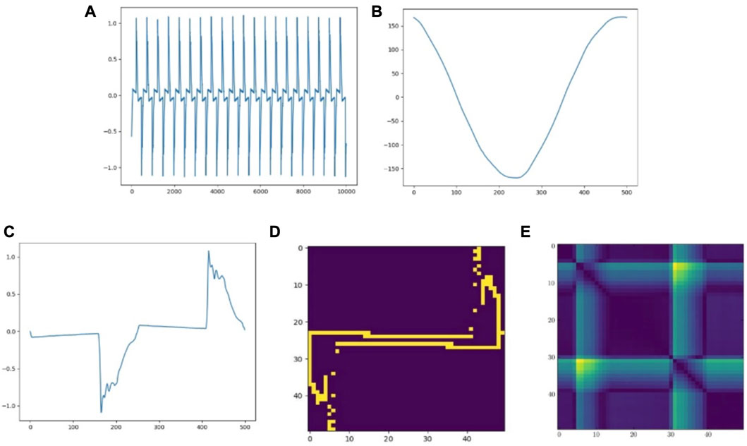
FIGURE 1. Extraction of current and voltage signals from the aggregated measurements. (A) Aggregate current. (B) Current waveform when CFL is turned on. (C) Voltage waveform when CFL is turned on. (D) V-I trajectory of CFL. (E) EDM of CFL.

In our experiments, we used a convolutional neural network to construct the structure shown in Figure 2 and trained the model using the V-I trajectories obtained from the PLAID to obtain a pre-trained convolutional neural network model capable of classifying V-I trajectory maps. The network contains five layers, including three convolutional layers and two fully connected layers, and ReLU is used as the activation function for each convolutional and fully connected layer. The first convolutional layer filters the input image with 16 kernels of size 5, straddling two pixels. The second convolutional layer takes the output of the first convolutional layer as the input and filters it with 32 kernels. The third convolutional layer filters it with 64 kernels of size 5. The role of the neural network is to perform feature extraction on the input data. The convolutional and fully connected layers of the pre-trained model can be considered as a cascade of feature extractors, and we carry out a separate process for the last fully connected layer for the purpose of fusing the DRO model, as follows:

1) All the layers except the last fully connected layer are extracted from the pre-trained model.

2) A fully connected layer combining the DRO model is linked to it.

3) Using V-I trajectory maps and the Euclidean distance matrix obtained from both datasets as the input, the last layer of the new network is separately trained until the stopping criterion is satisfied.

FIGURE 2

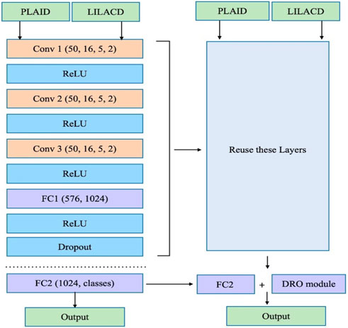
FIGURE 2. Structure of the network and addition of DRO modules.

It should be noted that in order to prevent the influence of the epoch of training sessions on the accuracy, we also carry out the same epoch of training for the pre-trained model as we did for the DRO model, so as to obtain the model without DRO added for the same epoch of training. We also performed several cross-validations of the data based on stratified sampling, and the final mean value was obtained as the final value.

As we derived previously, the empirical cross-entropy with the regularization term $‖{\mathit{W}}_m‖$ is an upper bound for the worst case of all distributions in the Wasserstein ball, $m\in \left[M\right]$, and since the empirical loss is still non-convex, it is suitable to use a local optimization method for the solution; we use a stochastic approximate gradient descent algorithm to adjust ${\mathit{W}}_m$, updated as follows:

${\mathit{W}}_m^{k+1}={\mathrm{p}\mathrm{r}\mathrm{o}\mathrm{x}}_{{\eta }_k\stackrel{\sim }{\lambda }‖{\mathit{W}}_m‖}\left({\mathit{W}}_m^k-{\eta }_k{\nabla }_{{\mathit{W}}_{\mathit{m}}}\mathcal{l}\left(h\left({\mathit{x}}^{{\mathit{i}}_{\mathit{k}}},y^{i_k}\right)\right)\right),$

where ${\eta }_k$ is the step size and ${\mathit{i}}_{\mathit{k}}$ is randomly selected from the index set $\left[N\right]$. According to Nitanda A (2014), the proximal operator of the convex function $\phi$ is defined as follows:

${\mathrm{p}\mathrm{r}\mathrm{o}\mathrm{x}}_{\phi }\left({\mathit{W}}_m\right):=\underset{{\mathit{W}}_m^{\prime }}{\mathrm{argmin}}\phi \left({\mathit{W}}_m^{\prime }\right)+\frac{1}{2}{‖{\mathit{W}}_m^{\prime }-{\mathit{W}}_m‖}_F^2,$

where ${‖\bullet ‖}_F$ stands for the Frobenius norm.

4.4 Results on the PLAID

On the PLAID, we first experimented with different initializations of the penalty coefficient, $\stackrel{\sim }{\lambda }$, for the regularization term. As shown in Figure 3, the hyperparameter $\stackrel{\sim }{\lambda }$ is $\left\{\mathrm{0,0.1,0.2,0.4},...,1.0\right\}$; 0 represents the neural network without adding the DRO model, and the remaining non-zero values represent the coefficient values of the penalty terms. It can be seen that the larger lambda values lead to an excessive upper bound on the approximation of the model, which weakens the differences between different appliances, thus leading to a lower classification performance. The classification accuracy of the model gradually decreases when the parameter is greater than $1$; when the parameter is around $0.6$, the model seems to gain stable performance, and the conclusions are roughly similar under both preprocessing methods.

FIGURE 3

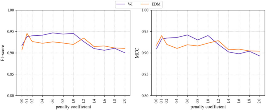
FIGURE 3. Effect of different penalty coefficients on the DRO model with PLAID data.

As a result, with the help of DRO, the F1-score of the PLAID improved from $0.9166\pm 0.023$ to $0.9261\pm 0.019$ and from $0.9065\pm 0.018$ to $0.9278\pm 0.018$ under the two preprocessing methods, respectively. In addition to which, we selected the CNN model from the literature (De Baets L et al., 2018) and the KNN method from the study by Gurbuz F B et al. (2021) to classify the appliance features, as shown in Table 1. Thus, it can be shown that the distributionally-robust optimization method effectively improves the classification ability of the network. For a more detailed analysis, we use the confusion matrix to visualize the classification of the proposed model. As shown in Figure 4, each row of the matrix represents the predicted labels; each category represents the true labels; the diagonal line indicates the number of each category correctly identified, i.e., the degree of matching between the predicted and true values; and the values outside the diagonal line indicate the portion of incorrect predictions.

TABLE 1

TABLE 1. Summary of the results of the two preprocessing methods combined with the DRO model under the PLAID.

FIGURE 4

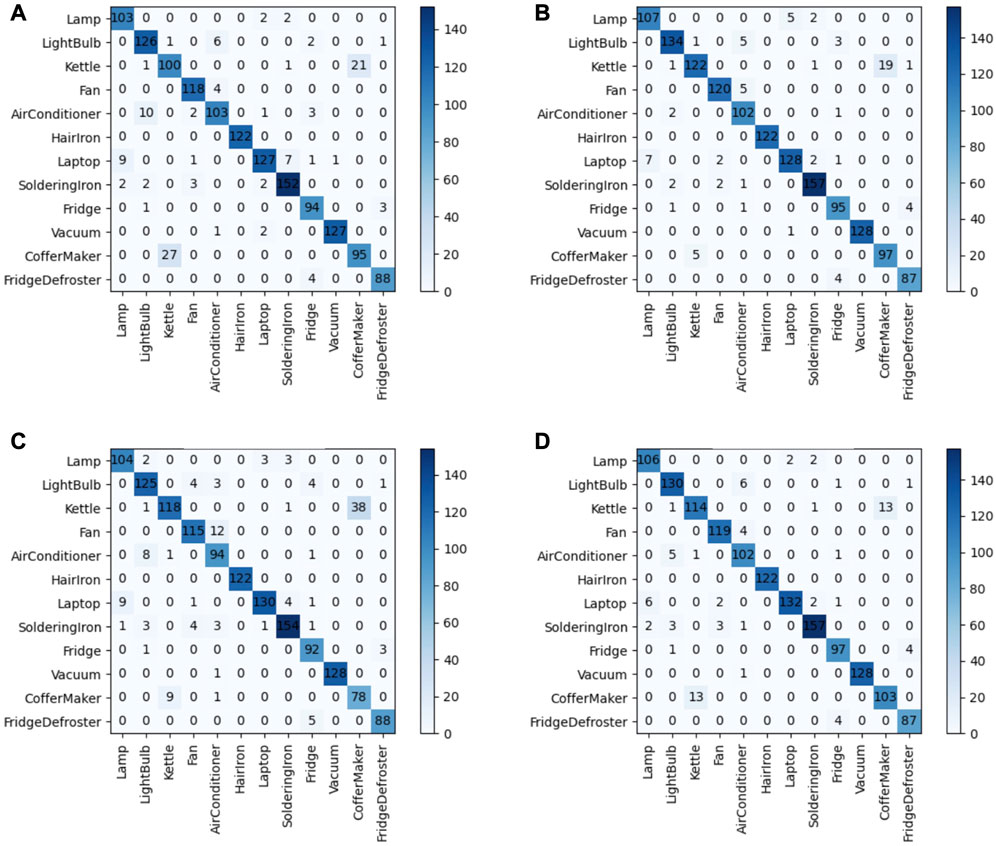
FIGURE 4. (A) V-I trajectory map without DRO addition. (B) V-I trajectory map with DRO addition. (C) Euclidean distance matrix without DRO addition. (D) Euclidean distance matrix with DRO addition.

4.5 Results on the LILACD

The LILACD contains the energy usage of some industrial and household electrical appliances, and we use the same steps as before while cross-validation is also applied. The addition of the DRO model is achieved by replacing the last layer of the pre-trained model. As a result, the network without DRO addition obtained an F1-score of $0.85\pm 0.061$ when using the V-I trajectory map as the input, while the model with DRO addition achieved an F1-score of $0.9058\pm 0.077$; SVM (Hernandez A S et al., 2021) achieved an F1-score of $0.787\pm 0.091$, and KNN obtained an F1-score of $0.77\pm 0.07$. When using the Euclidean distance matrix to represent the appliance features, the model with DRO addition achieved an F1-score of $0.87\pm 0.025$, which is about $5\%$ higher than the model without DRO addition and 15% higher than the traditional machine learning methods, SVM and KNN. To evaluate the classification performance of each appliance, Figure 5 and Figure 6 show the detailed F1-score for each appliance. It can be seen that the DRO model achieves more significant results in the classification of coffee machines, hair dryers, kettles, and raclettes, mainly because of the irregular fluctuating waveforms of the appliance, which made the accuracy significantly lower. These devices are similar in that they all work in the form of the generated heat energy, resulting in variable device states, while the different gears directly affect the final power output, making it difficult to identify methods with a low robustness.

FIGURE 5

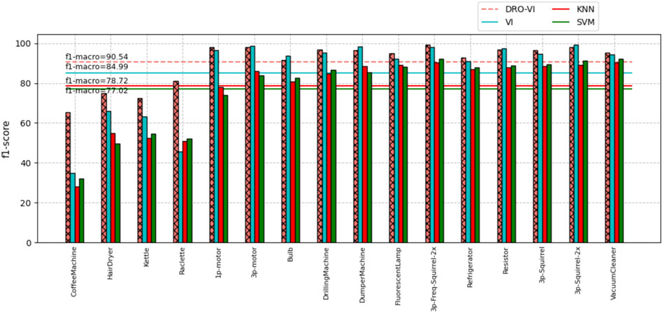
FIGURE 5. F1-score of appliance loads for the LILACD with the V-I trajectory.

FIGURE 6

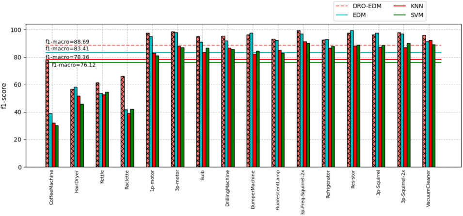
FIGURE 6. F1-score of appliance loads for the LILACD with EDM.

Overall, these results indicate that the DRO model significantly improves robustness performance, allowing the network to cope well with irregular fluctuations in equipment and to achieve high accuracy in both residential and industrial equipment classifications.

5 Conclusion and future work

In this paper, we propose a Wasserstein metric-based distributionally robust optimization framework for the non-intrusive load monitoring problem and establish a relationship between robustness and regularization in multiple variables by reformulating the min–max problem as a regularized empirical loss minimization problem through multiple upper approximations. In addition, two appliance feature extraction methods for high-frequency load data are used in the experiments to investigate the effect of the DRO method on the performance of the neural network when the convolutional neural network has different input data. In addition, the proposed DRO module can be added to the single-layer neural network in the form of constraints to improve the network performance. Experiments show that the proposed method has better robustness for devices with large fluctuations and can effectively identify device features compared to the network without DRO. Since there is no method that can directly solve the proposed DRO model, more accurate solution methods will be the focus of research in the future.

Data availability statement

The original contributions presented in the study are included in the article/Supplementary Material; further inquiries can be directed to the corresponding author.

Author contributions

QZ: conceptualization, methodology, formal analysis, writing—original draft, writing—review and editing, and visualization. YY: resources and writing—review and editing. FK: supervision and project administration. SC: methodology and validation. LY: supervision, writing—review and editing, and funding acquisition.

Funding

This work was supported by the Natural Science Foundation of Guangxi (2020GXNSFAA297173 and 2020GXNSFDA238017), the Natural Science Foundation of China (51767003), the Thousands of Young and Middle-Aged Backbone Teachers Training Program for Guangxi Higher Education [Education Department of Guangxi (2017)], and the Innovation Project of Guangxi Graduate Education (YCSW2022050).

Conflict of interest

The authors declare that the research was conducted in the absence of any commercial or financial relationships that could be construed as a potential conflict of interest.

The handling editor DZ declared a shared affiliation with the authors at the time of the review.

Publisher’s note

All claims expressed in this article are solely those of the authors and do not necessarily represent those of their affiliated organizations, or those of the publisher, the editors, and the reviewers. Any product that may be evaluated in this article, or claim that may be made by its manufacturer, is not guaranteed or endorsed by the publisher.

References

Abd El-Ghany, H. A., Elgebaly, A. E., and Taha, I. B. M. (2021). A new monitoring technique for fault detection and classification in PV systems based on rate of change of voltage-current trajectory. Int. J. Electr. Power and Energy Syst. 133, 107248. doi:10.1016/j.ijepes.2021.107248

CrossRef Full Text | Google Scholar

Asensio, M., and Contreras, J. (2015). Stochastic unit commitment in isolated systems with renewable penetration under CVaR assessment. IEEE Trans. Smart Grid 7 (3), 1356–1367. doi:10.1109/tsg.2015.2469134

CrossRef Full Text | Google Scholar

Azizi, E., Beheshti, M. T. H., and Bolouki, S. (2021). Event matching classification method for non-intrusive load monitoring. Sustainability 13 (2), 693. doi:10.3390/su13020693

CrossRef Full Text | Google Scholar

Chea, R., Thourn, K., and Chhorn, S. “Improving VI trajectory load signature in NILM spproach,” in Proceedings of the 2022 International Electrical Engineering Congress (iEECON), Khon Kaen, Thailand, March 2022, 1–4.

Google Scholar

Cheramin, M., Cheng, J., Jiang, R., and Pan, K. (2022). Computationally efficient approximations for distributionally robust optimization under moment and Wasserstein ambiguity. Inf. J. Comput. 34 (3), 1768–1794. doi:10.1287/ijoc.2021.1123

CrossRef Full Text | Google Scholar

De Baets, L., Dhaene, T., Deschrijver, D., Develder, C., Berges, M., et al. (2018b). “VI-based appliance classification using aggregated power consumption data,” in Proceedings of the 2018 IEEE international conference on smart computing (SMARTCOMP), Taormina, Italy, June 2018 (IEEE), 179–186. doi:10.1109/SMARTCOMP.2018.00089

CrossRef Full Text | Google Scholar

De Baets, L., Ruyssinck, J., Develder, C., Dhaene, T., and Deschrijver, D. (2018a). Appliance classification using VI trajectories and convolutional neural networks. Energy Build. 158, 32–36. doi:10.1016/j.enbuild.2017.09.087

CrossRef Full Text | Google Scholar

Defourny, B. (2010). “Machine learning solution methods for multistage stochastic programming,”. PhD diss (Belgium, Europe: University of Liege). https://www.lehigh.edu/defourny/PhDthesis_B_Defourny.pdf.

Google Scholar

Delage, E., and Ye, Y. (2010). Distributionally robust optimization under moment uncertainty with application to data-driven problems. Operations Res. 58 (3), 595–612. doi:10.1287/opre.1090.0741

CrossRef Full Text | Google Scholar

Dokmanic, I., Parhizkar, R., Ranieri, J., and Vetterli, M. (2015). Euclidean distance matrices: Essential theory, algorithms, and applications. IEEE Signal Process. Mag. 32 (6), 12–30. doi:10.1109/msp.2015.2398954

CrossRef Full Text | Google Scholar

Du, L., He, D., Harley, R. G., and Habetler, T. G. (2015). Electric load classification by binary voltage–current trajectory mapping. IEEE Trans. Smart Grid 7 (1), 358–365. doi:10.1109/tsg.2015.2442225

CrossRef Full Text | Google Scholar

Duan, C., Fang, W., Jiang, L., Yao, L., and Liu, J. (2018). Distributionally robust chance-constrained approximate AC-OPF with Wasserstein metric. IEEE Trans. Power Syst. 33 (5), 4924–4936. doi:10.1109/tpwrs.2018.2807623

CrossRef Full Text | Google Scholar

Everett, H. (1963). Generalized Lagrange multiplier method for solving problems of optimum allocation of resources. Operations Res. 11 (3), 399–417. doi:10.1287/opre.11.3.399

CrossRef Full Text | Google Scholar

Gao, J., Giri, S., Kara, E. C., and Bergés, M. “Plaid: A public dataset of high-resoultion electrical appliance measurements for load identification research: Demo abstract,” in Proceedings of the 1st ACM Conference on Embedded Systems for Energy-Efficient Buildings, Memphis, TN, USA, November 2014, 198–199.

Google Scholar

Gillis, J. M., Chung, J. A., and Morsi, W. G. (2017). Designing new orthogonal high-order wavelets for nonintrusive load monitoring. IEEE Trans. Industrial Electron. 65 (3), 2578–2589. doi:10.1109/tie.2017.2739701

CrossRef Full Text | Google Scholar

Gouk, H., Frank, E., Pfahringer, B., and Cree, M. J. (2021). Regularisation of neural networks by enforcing Lipschitz continuity. Mach. Learn. 110, 393–416. doi:10.1007/s10994-020-05929-w

CrossRef Full Text | Google Scholar

Gurbuz, F. B., Bayindir, R., and Vadi, S. “Comprehensive non-intrusive load monitoring process: Device event detection, device feature extraction and device identification using KNN, random forest and decision tree,” in Proceedings of the 2021 10th International Conference on Renewable Energy Research and Application (ICRERA), Istanbul, Turkey, September 2021, 447–452.

Google Scholar

Hart, G. W. (1992). Nonintrusive appliance load monitoring. Proc. IEEE 80 (12), 1870–1891. doi:10.1109/5.192069

CrossRef Full Text | Google Scholar

Hernandez, A. S., Ballado, A. H., and Heredia, A. P. D. “Development of a non-intrusive load monitoring (nilm) with unknown loads using support vector machine,” in Proceedings of the 2021 IEEE International Conference on Automatic Control and Intelligent Systems (I2CACIS), Shah Alam, Malaysia, June 2021, 203–207.

Google Scholar

Kahl, M., Krause, V., Hackenberg, R., Ul Haq, A., Horn, A., Jacobsen, H. A., et al. (2019). Measurement system and dataset for in-depth analysis of appliance energy consumption in industrial environment. Tm-Technisches Mess. 86 (1), 1–13. doi:10.1515/teme-2018-0038

CrossRef Full Text | Google Scholar

Liu, Y., Wang, X., and You, W. (2018b). Non-intrusive load monitoring by voltage–current trajectory enabled transfer learning. IEEE Trans. Smart Grid 10 (5), 5609–5619. doi:10.1109/tsg.2018.2888581

CrossRef Full Text | Google Scholar

Liu, Y., Wang, X., Zhao, L., and Liu, Y. (2018a). Admittance-based load signature construction for non-intrusive appliance load monitoring. Energy Build. 171, 209–219. doi:10.1016/j.enbuild.2018.04.049

CrossRef Full Text | Google Scholar

Lu, J., Zhao, R., Liu, B., Yu, Z., Zhang, J., and Xu, Z. (2023). An overview of non-intrusive load monitoring based on V-I trajectory signature. Energies 16 (2), 939. doi:10.3390/en16020939

CrossRef Full Text | Google Scholar

Makonin, S., and Popowich, F. (2015). Nonintrusive load monitoring (NILM) performance evaluation: A unified approach for accuracy reporting. Energy Effic. 8, 809–814. doi:10.1007/s12053-014-9306-2

CrossRef Full Text | Google Scholar

Nitanda, A. (2014). Stochastic proximal gradient descent with acceleration techniques. Adv. Neural Inf. Process. Syst. 27.

Google Scholar

Rahimian, H., and Mehrotra, S. (2019). Distributionally robust optimization: A review. arXiv preprint arXiv:1908.05659 https://arxiv.org/abs/1908.05659.

Google Scholar

Wan, L., Zeiler, M., Zhang, S., Le Cun, Y., and Fergus, R. “Regularization of neural networks using dropconnect,” in Proceedings of the International conference on machine learning, Atlanta, Georgia, USA, June 2013 (PMLR), 1058–1066.

Google Scholar

Wang, A. L., Chen, B. X., Wang, C. G., and Hua, D. (2018). Non-intrusive load monitoring algorithm based on features of V–I trajectory. Electr. Power Syst. Res. 157, 134–144. doi:10.1016/j.epsr.2017.12.012

CrossRef Full Text | Google Scholar

Wei, W., Liu, F., Mei, S., and Hou, Y. (2014). Robust energy and reserve dispatch under variable renewable generation. IEEE Trans. Smart Grid 6 (1), 369–380. doi:10.1109/tsg.2014.2317744

CrossRef Full Text | Google Scholar

Xie, H., Jiang, M., Zhang, D., Goh, H. H., Ahmad, T., Liu, H., et al. (2023). IntelliSense technology in the new power systems. Renew. Sustain. Energy Rev. 177, 113229. doi:10.1016/j.rser.2023.113229

CrossRef Full Text | Google Scholar

Yoon, S. H., Kim, S. Y., Park, G. H., Kim, Y. K., Cho, C. H., and Park, B. H. (2018). Multiple power-based building energy management system for efficient management of building energy. Sustain. Cities Soc. 42, 462–470. doi:10.1016/j.scs.2018.08.008

CrossRef Full Text | Google Scholar

Zhang, D., Zhu, H., Zhang, H., Goh, H. H., Liu, H., and Wu, T. (2021). Multi-objective optimization for smart integrated energy system considering demand responses and dynamic prices. IEEE Trans. Smart Grid 13 (2), 1100–1112. doi:10.1109/tsg.2021.3128547

CrossRef Full Text | Google Scholar

Zhao, C., and Guan, Y. (2018). Data-driven risk-averse stochastic optimization with Wasserstein metric. Operations Res. Lett. 46 (2), 262–267. doi:10.1016/j.orl.2018.01.011

CrossRef Full Text | Google Scholar

Zheng, Z., Chen, H., and Luo, X. (2018). A supervised event-based non-intrusive load monitoring for non-linear appliances. Sustainability 10 (4), 1001. doi:10.3390/su10041001

CrossRef Full Text | Google Scholar