Regional electricity market price forecasting based on an adaptive spatial–temporal convolutional network

The accurate prediction of electricity prices has great significance for the power system and the electricity market, regional electricity prices are difficult to predict due to congestion issues in regional transmission lines. A regional electricity price prediction framework is proposed based on an adaptive spatial–temporal convolutional network. The proposed framework is expected to better explore regional electricity prices’ spatial–temporal dynamic characteristics in the electricity spot market and improve the predictive accuracy of regional electricity prices. First, different areas of the electricity market are regarded as nodes. Then, each area’s historical electricity price data are used as the corresponding node’s characteristic information and constructed into a graph. Finally, a graph containing the spatial–temporal information on electricity prices is input to the adaptive spatial–temporal prediction framework to predict the regional electricity price. Operational data from the Australian electricity market are adopted, and the prediction results from the proposed adaptive spatial–temporal prediction framework are compared with those of existing methods. The numerical example results show that the predictive accuracy of the proposed framework is better than the existing baseline and similar methods. In the twelve-step forecast example in this paper, considering the spatial dependence of the spot electricity price can improve the forecast accuracy by at least 10.3% and up to 19.8%.

1 Introduction

Against the backdrop of the ongoing global low-carbon transformation, electricity markets have received widespread attention, playing an essential role in improving electricity use efficiency and optimizing power resource allocation. More than 30 countries and regions currently have electricity markets, and many developing countries have begun to explore and establish electricity market systems (Tan et al., 2018). The accurate prediction of electricity prices has great significance for the power system and the electricity market, supports the safe and stable operation of the power system, and provides optimal trading strategy guidance for market participants. From the existing electricity market’s perspective, the spot market’s electricity price fluctuates widely and is easily affected by the relationship between supply and demand, emergencies, environmental changes, bidding strategies, and renewables (Yang et al., 2021). Therefore, the accurate prediction of electricity prices has received significant attention from researchers (Jin et al., 2021).

Most of the present research on electricity price prediction is based on the time dimension. More specifically, the electricity price prediction issue is treated as a time-series prediction problem, and methods such as statistical models, machine learning, and deep learning are used to deal with the time-series prediction issue.

Statistical models are applied to electricity price prediction and have strong generality and interpretability. Chitsaz et al. (2018) used the autoregressive model with the exogenous variables (ARX) model to predict the electricity price, while a new Hilbertian autoregressive moving average with exogenous inputs (ARMAX) model for electricity price forecasting was proposed by Portela et al. (2016). Uniejewski et al. (2017) introduced the seasonal component autoregressive model, and the quantile regression average model was introduced to forecast the day-ahead electricity price, further improving the forecasting accuracy. Statistical models perform well in stable scenarios but have limited ability to predict electricity prices with large randomness, strong nonlinearity, and non-stationarity.

Rapidly developing machine learning approaches have also been applied to electricity price prediction. Wan et al. (2017) proposed an extreme learning machine and a non-dominated sorting genetic algorithm II (NSGA-II) Pareto optimal-prediction-interval construction method. Wei et al. (2021) applied the random forest regression algorithm to spot market clearing price prediction, obtaining a 25% improvement compared with a baseline algorithm; Hafeez et al. (2021) proposed an integrating feature engineering (FE) and modified firefly optimization (mFFO) algorithm with SVR method to improve computational efficiency and optimal parameter adjustment in load forecasting. Hafeez et al. (2020a) proposed a day-ahead gray wolf modified enhanced differential evolution algorithm (DA-GmEDE) based home energy management controller (HEMC), the energy management strategy proposed in this document has improved by 33.3% compared with the baseline strategy. Hafeez et al. (2020b), a fast and accurate short-term load forecasting model is proposed. The abstractive features from the historical data are extracted using modified mutual information (MMI) technique. The factored conditional restricted Boltzmann machine (FCRBM) is empowered via learning to predict the electric load. Eventually, the proposed genetic wind driven optimization (GWDO) algorithm is used to optimize the performance. The remarkable advantages of the proposed framework are the improved forecast accuracy and convergence rate. Because local electricity price prediction is often affected by dynamic electricity price changes in neighboring areas, Xiao et al. (2021) considered a new online sequential extreme learning machine algorithm to improve electricity price prediction results. Tschora et al. (2022) studied the effect of different machine learning methods in predicting electricity prices, considering the historical prices of neighboring countries to improve the prediction results. Because of the many influencing factors involved in electricity prices, traditional methods still cannot fully characterize them, so the predictive accuracy was limited (Luo et al., 2022).

Deep learning has received increasing research attention recently and has been widely used in electricity price forecasting (Niet et al., 2021). Lago et al. (2018) proposed four deep learning models to predict electricity prices while comparing and analyzing the accuracy of 27 common electricity price prediction methods. The results showed that deep learning methods generally have better accuracy than statistical models. Afrasiabi et al. (2019) applied wind speed and residential load forecasts as auxiliary inputs for electricity price prediction and proposed a deep learning algorithm to estimate the probability density of electricity prices. Zhang et al. (2020) proposed an adaptive hybrid model based on variational mode decomposition (VMD), self-adaptive particle swarm optimization (SAPSO), seasonal autoregressive integrated moving average (SARIMA) network, and deep belief network (DBN) to predict electricity market prices.

Qiao et al. (2020) proposed a hybrid electricity price prediction model based on wavelet transform-stacked autoencoder-LSTM (long short-term memory). Deng et al. (2021) used a deep learning-based man-hour cycle and multi-step price forecasting model to improve forecasting performance by capturing steep price changes. Jahangir et al. (2021) proposed the micro-clustering and bidirectional LSTM prediction method to forecast wind speed, load, and electricity prices in different periods. Toubeau et al. (2021) employed a deep bidirectional LSTM for probabilistic prediction of distributed node marginal prices to capture complex temporal dynamics. Lu et al. (2022) designed a conditional time series generative adversarial network (TSGAN) to predict electricity prices after data preprocessing and conditional selection.

In the studies described above, the essence of electricity price forecasting is a single time series prediction without considering the potential spatial influence of electricity prices in other regions. In the past few years, some investigators have proposed exploring the spatial dependence of electricity prices in different regions to improve predictive accuracy. Abate et al. (2017) derived a price–space model with temporal and spatial lags. Statistical tests showed that the electricity price across regions has a significant spatial dependence, that is as important as the time dependence. Han et al. (2022) proposed a network LSTM algorithm based on graph convolution. A graph convolutional neural network was used to mine spatial information, and LSTM was used to mine temporal information to predict marginal electricity prices. Yang et al. (2022) developed a prediction model based on the attention-based spatial–temporal graph convolutional network and designed a three-branch network structure to match the compositional structure of the node marginal electricity price.

Existing spatial–temporal prediction methods for electricity prices do not explain how to solve the problem of prior edge knowledge, that is, how to define the adjacency matrix of the input model. The adjacency matrix A can be set to a corresponding static value. For example, it can be predefined by physical adjacency information, functional similarity information, and connectivity information (Geng et al., 2019). However, it is difficult to quantitatively predefine the adjacency information of different regional electricity prices in practice. Solving this problem is the key to graph neural network (GNN) exploration of the spatial dependence of electricity prices in different regions.

This paper proposes a regional electricity price prediction framework based on an adaptive spatial–temporal convolutional network to solve the above problems. First, different regions in the electricity market are regarded as nodes. Then each region’s historical electricity price data are considered the node features and constructed into a graph. Finally, the graph containing electricity price spatial–temporal information is input into the adaptive spatial–temporal prediction framework to predict the regional electricity price. The adaptive adjacency matrix is adopted within the spatial–temporal prediction framework to solve the problem of absent prior edge knowledge.

The main contributions of this paper are:

(1) Unlike existing work, the proposed regional electricity price prediction framework applies a temporal convolutional network to mine the time-dimensional information of regional electricity prices. It considers the potential spatial influence of electricity prices in other regions while using a graph convolutional network to mine its potential. Based on the spatial dynamics of the temporal characteristics, the spatial characteristics are used to improve the predictive accuracy of regional electricity prices.

(2) The adaptive adjacency matrix enables the GNN to mine the spatial characteristic information of regional electricity prices without prior knowledge of edges, reducing the complexity of the required data.

(3) The predictive accuracy is significantly improved compared with existing baseline and similarity-working methods.

2 Graph neural networks and temporal convolution network

2.1 Graph neural networks

2.1.1 Graph neural networks

In recent years, graph neural networks (GNNs) have achieved good results in tasks related to graph-structured data. They have been widely used in many fields, such as social networks, knowledge graphs, molecular chemistry, and life sciences (Wang et al., 2021a). The advantages of GNNs have been demonstrated in detecting and locating faults in distribution networks, power system stability, and other issues, and they have been widely used in other power field areas (Sun et al., 2022). Graph structural data is divided into Euclidean and non-Euclidean structural data. Figure 1A shows Euclidean structure data with a fixed arrangement order, and Figure 1B shows non-Euclidean structure data with no fixed arrangement order. A convolutional neural network (CNN) has difficulty defining convolution kernels for non-Euclidean structural data, while a GNN can handle non-Euclidean structural data well (Xu et al., 2020).

FIGURE 1

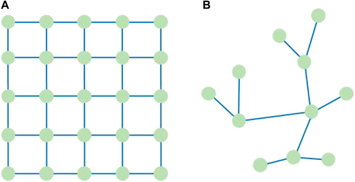
FIGURE 1. Two kinds of graph structure data. (A) Euclid structural data. (B) Non euclid structural data.

Graph $G=\left(V,E\right)$ is composed of groups of nodes V and edges E, where $v_i\in V$ represents the ith node in graph G, and $e_{ij}\in E$ is an edge from node $v_i$ to node $v_j$ in graph G. The adjacency matrix A describes the adjacent relationship between nodes in graph G. A is an $N\times N$ matrix, and N is the total number of nodes. If $e_{ij}\in E$ then $A_{ij}=1$, and if $e_{ij}\notin E$, then $A_{ij}=0$. Node V in graph G can also have the feature $X\in {\mathbb{R}}^{N\times D}$, where X is the characteristic matrix of the node, $X_{ij}\in R^{1\times D}$ is the feature vector of node $v_i$, and D is the total number of node features.

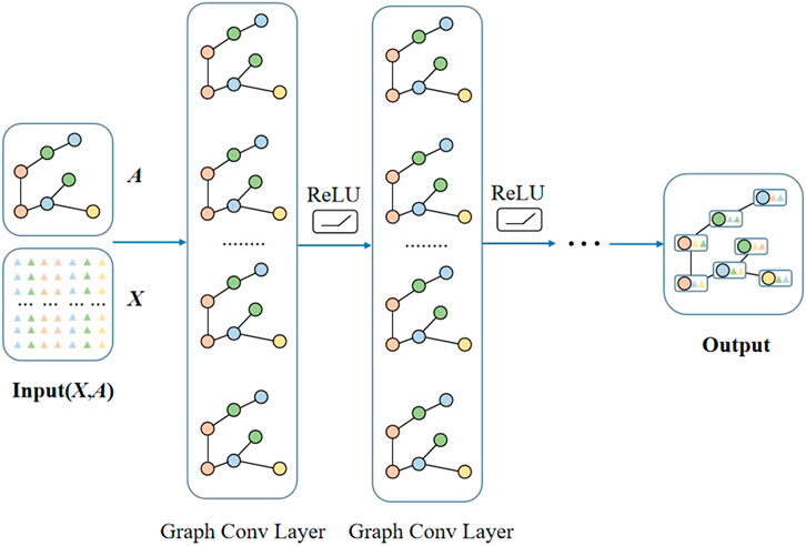
Graph convolutional networks (GCNs) can extract features from graph-structured data and be combined with other neural networks. GCNs can be divided into networks based on spectral and spatial domain methods. The method based on the spectral domain converts the data for processing from the spatial domain to the spectral domain according to spectral theory and the convolution theorem. The method based on the spatial domain defines convolution operations directly in space, updating by convolving the representations of the center and neighbor nodes. The method based on the spatial domain is more efficient and flexible and has received extensive attention in recent years. The graph convolutional network structure diagram is shown in Figure 2.

FIGURE 2

FIGURE 2. Graph convolutional network structure diagram.

Graph convolution from a diffusion convolutional neural network is based on the spatial graph convolution method (Atwood et al., 2016). It is regarded as a diffusion process in which information is transferred between adjacent nodes with a particular transition probability. Assuming that the equilibrium of the information distribution is reached after multiple diffusion steps, it is defined as (Atwood et al., 2016):

$H_k=W_{k}e{Z}_{k}X(1)$

where $Z_k=\frac{A}{rowsum\left(A\right)}\in {\mathbb{R}}^{N\times N}$ is the probability transferring matrix, k is the kth diffusion step, e represents the product of the elements of two matrices, $H_k$ indicates the hidden output of the kth diffusion step, $W_k\in {\mathbb{R}}^{D\times M}$ represents the learnable weight corresponding to the kth diffusion step, and M is the number of matrix columns. The hidden outputs $H_k$ of the diffusion steps are independent of each other, and the final graph convolution output is obtained by accumulating all hidden outputs from a finite number of diffusion steps (Li et al., 2018):

$\mathit{U}={\displaystyle \sum _{\mathit{k}=0}^{{\mathit{K}}_{\mathit{a}}}}{\mathit{Z}}_{\mathit{k}}\mathit{X}{\mathit{W}}_{\mathit{k}}(2)$

where $U\in {\mathbb{R}}^{N\times M}$ is the final graph convolution output, and $K_a$ denotes the total number of diffusion steps.

2.1.2 Graph adjacency matrix

There are many ways to construct the GNN adjacency matrix A (Geng et al., 2019). When the information between nodes in the graph is known a priori, the adjacency matrix A can be set to a corresponding static value through physical adjacency information, functional similarity information, and connectivity information to predetermine the adjacency matrix (Geng et al., 2019). Other approaches involve building a dynamic adjacency matrix in the graph training process, such as learning and updating the weights of adjacent nodes using an attention mechanism, Gaussian kernel, or adaptive path layer method, but these still require a predefined graph structure.

In regional electricity price prediction, it is difficult to quantitatively predetermine the adjacency information relationship between different regions and obtain the adjacency information relationship data. This paper solves this problem by adopting an adaptive adjacency matrix with learnable ability. This electricity price spatial–temporal prediction framework for learning and mining potential dynamic spatial dependencies is expected to improve the accuracy of the prediction model. The adaptive adjacency matrix ${\stackrel{\sim }{A}}_{adp}$ is

${\stackrel{\sim }{A}}_{adp}=\mathrm{S}\mathrm{o}\mathrm{f}\mathrm{t}\mathrm{m}\mathrm{a}\mathrm{x}\left(\mathrm{R}\mathrm{e}\mathrm{L}\mathrm{U}\left(E_1{E}_2^T\right)\right)(3)$

In Eq. 3, $\mathrm{S}\mathrm{o}\mathrm{f}\mathrm{t}\mathrm{m}\mathrm{a}\mathrm{x}$ and $\mathrm{R}\mathrm{e}\mathrm{L}\mathrm{U}$ are activation functions. $E_1$ and $E_2$ denote the source and the target node embedding, respectively (Goyal et al., 2017), where the node embedding can be learned and randomly initialized. The adaptive adjacency matrix ${\stackrel{\sim }{A}}_{adp}$ is considered a transfer matrix in the hidden diffusion process. An alternative to the probability transition matrix is given by Eq. 2. Therefore, this method can perform graph convolution when prior knowledge cannot determine the spatial dependencies between nodes.

2.2 Temporal convolution networks

2.2.1 Temporal convolution network

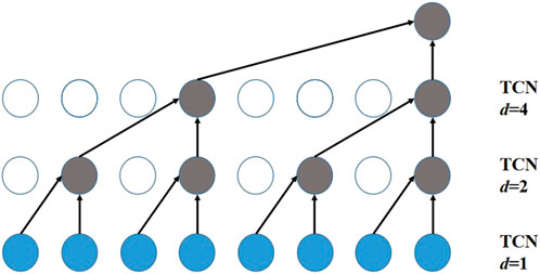
This paper uses a dilated causal convolution as a temporal convolution network (TCN) to mine the nodal temporal dimension information. Dilated causal convolution enables an exponential increase in the receptive field by increasing the hidden layer depth. Unlike recurrent neural network (RNN) methods, dilated causal convolution can process long sequences in a non-recursive manner, facilitating parallel computation and alleviating the problem of exploding gradients. Dilated causal convolution preserves causal order in time by padding the input with zeros, so predictions for the current time step involve only historical data. Dilated causal convolution, a special case of standard one-dimensional convolution, slides the input by skipping values at a particular step, as shown in Figure 3.

FIGURE 3

FIGURE 3. Dilated causal convolution.

Given a one-dimensional sequence of inputs $B\in {\mathbb{R}}^T$ and a filter $f\in {\mathbb{R}}^K$, dilated causal convolution between B and f at time t is expressed as:

$B*f\left(t\right)={\displaystyle \sum _{s=0}^{K-1}}f\left(s\right)B\left(t-d\times s\right)(4)$

In Eq. 4, K is the kernel size, d is the dilated factor controlling the jump distance, s is the kernel number, and T is the step size. By incrementally stacking the dilated causal convolution layer with a dilated factor, the receptive field of the model increases exponentially so that the dilated causal convolution network can mine longer sequences with fewer layers.

2.2.1 Gated temporal convolutional network

The simplest gated temporal convolutional network (gated TCN) contains only one output gate h. Then, given input $P\in {\mathbb{R}}^{N\times D\times T}$, its operation is expressed as:

$h=\mathrm{g}\left({\mathrm{\Theta }}_1*P+b\right)\odot \sigma \left({\mathrm{\Theta }}_2*P+c\right)(5)$

where ${\mathrm{\Theta }}_1$, ${\mathrm{\Theta }}_2$, b and c are the model parameters, g is the output activation function, and $\sigma$ represents an S-type function. The model in this paper uses a gated TCN to mine complex time series and sets the activation function as a hyperbolic tangent function based on experience.

3 Regional electricity price forecasting framework based on an adaptive spatial–temporal convolution network

3.1 Constructing a spatial–temporal infographic with regional electricity prices

The increasing frequency of cross-regional power market transactions and long-distance power transmission affects electricity price fluctuations in different regions. There is a potential spatial dependence of power flow between different regions in the power market that previous prediction algorithms based on time series have difficulty describing accurately. Unlike traditional electricity price forecasting, the regional electricity price forecasting proposed in this paper trains a model containing regional electricity price information. In addition to mining the time dimension of regional electricity price information, it also mines the potential spatial dependencies between regions to improve predictive accuracy.

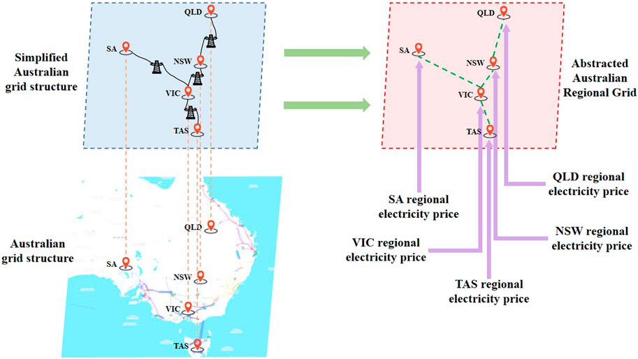
The data-driven regional electricity price forecast in the time and space dimensions can be regarded as a multivariate time series prediction problem with related spatial dependencies. As shown in Figure 4, different areas in the electricity market are first regarded as nodes to construct a spatial–temporal information map of regional electricity prices. Then, each area’s historical electricity price data is used as the node’s characteristic information. Finally, each node is constructed into a picture.

FIGURE 4

FIGURE 4. Spatial-temporal infographic of regional electricity prices.

Let $X_t=\left[x_{1,t},\cdots ,x_{N,t}\right]$ be the historical characteristic values, where $x_{i,t}=\left[x_{i,1,t},\cdots ,x_{i,t,D}\right]$ denotes the D characteristic values of the ith node at time t. Thus, the dataset of N nodes with T time steps can be represented as a three-dimensional array $\left[x_1,\cdots ,x_T\right]\in {\mathbb{R}}^{N\times T\times D}$.

The regional price is combined into a graph structure by regarding each power market region as a node, and the grid connectivity information between regions is described as edges. Graph $G_L=\left(V_L,E_L\right)$ is used to represent the graph structure of regional electricity prices, where $V_L$ is the set of all regional nodes and $E_L$ is the set of edges between regions.

According to the above definition, a graph $G_L$ is composed of N regional nodes. The regional electricity price prediction with H steps (prediction based on the last H steps of historical data) can be expressed as a learning function $f:{\mathbb{R}}^{N\times H\times D}⟶{\mathbb{R}}^{N\times 1\times D}$ that maps the historical data $\left\{X_{t-H+1},\cdots ,X_t\right\}$ to the regional electricity price of N nodes in the next time step t+1, namely,

$\left\{X_{t-H+1},\cdots ,X_t,G_L\right\}{\stackrel{f\left(\bullet \right)}{{\displaystyle \to }}X}_{t+1}(6)$

where $\left\{X_{t-H+1},\cdots ,X_t\right\}\in {\mathbb{R}}^{N\times H\times D}$, $X_{t+1}\in {\mathbb{R}}^{N\times 1\times D}$, and $X_{t+1}$ are the data of D characteristics of the N area nodes at time t+1.

3.2 Graph convolutional layers with adaptive adjacency matrix

As discussed earlier, it is challenging to quantitatively predetermine and obtain the adjacency information relationship of electricity prices in different regions. This paper adopts an adaptive adjacency matrix ${\stackrel{\sim }{A}}_{adp}$ with a learnable ability to solve this problem of describing regional nodes connectivity. This approach reduces the complexity of data requirements while ensuring prediction accuracy.

For the adaptive adjacency matrix, the random gradient descent method is used for point-to-point learning without prior knowledge of edges (see Eq. 3 for the definition of the adaptive adjacency matrix). The two learnable parameters $E_1,E_2\in {\mathbb{R}}^{N\times C}$ are initialized randomly, where C is the super parameter of the node embedding size. The spatial dependency weight between the source node and the target node is obtained by multiplying $E_1$ and $E_2$. By replacing the transition matrix Z in Eq. 2 with the adaptive adjacency matrix ${\stackrel{\sim }{A}}_{adp}$, the graph convolution output with the adaptive adjacency matrix is obtained:

$U={\displaystyle \sum _{k=0}^{K_a}}{\stackrel{\sim }{A}}_{adp}X{W}_k(7)$

3.3 Adaptive spatial–temporal prediction framework

The adaptive spatial–temporal prediction framework mines the latent spatial dependencies between different nodes without prior knowledge of edges through an adaptive adjacency matrix (Wu et al., 2019). This paper proposes an adaptive spatial–temporal prediction framework to predict regional electricity prices in the electricity market. The overall framework is shown in Figure 5. It consists of three main modules: a graph convolutional layer (GCL) with an adaptive adjacency matrix, gated temporal convolutional networks (gated TCNs), and a spatial–temporal prediction framework.

FIGURE 5

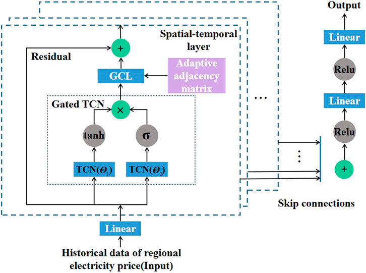
FIGURE 5. Regional electricity price forecasting framework based on adaptive spatial-temporal convolutional network.

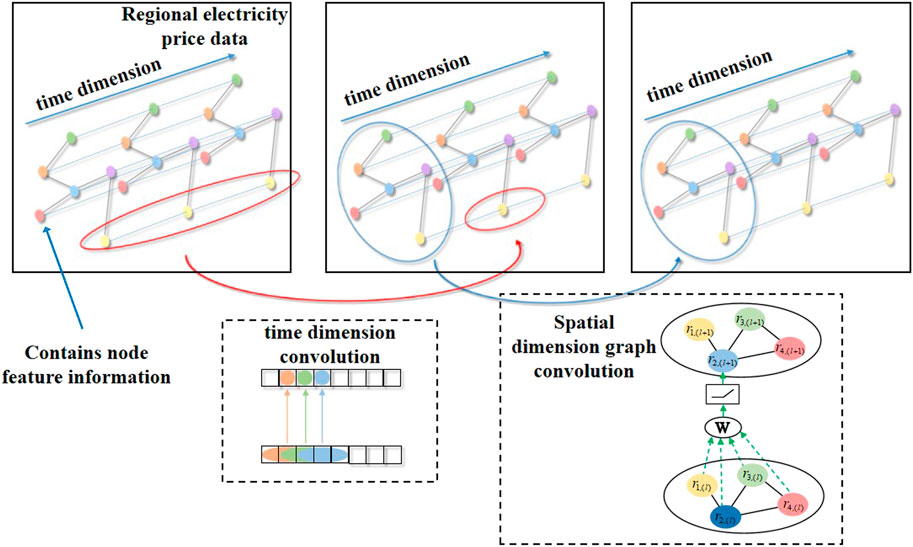
Figure 5 shows that multiple spatial–temporal layers are superimposed after the spatial–temporal information is extracted through the GCL–TCN layer (Wu et al., 2019). The framework uses a skip connection mechanism to handle spatial dependencies at different temporal levels (Wu et al., 2019). For a spatial–temporal layer, historical data is processed and input into the gated TCN and then into the GCL. The adjacency matrix in the GCL is the proposed adaptive adjacency matrix.

Figure 6 shows a schematic diagram of the GCL–TCN layer in which the principle of graph convolution is illustrated to help readers to understand it more intuitively. In this figure, $r_{1,\left(l+1\right)}$, $r_{2,\left(l+1\right)}$$r_{3,\left(l+1\right)},$ and $r_{4,\left(l+1\right)}$ are the characteristic values of the first, second, third, and fourth node $\left(l+1\right)$ layers, respectively, and $r_{1,\left(l\right)}$, $r_{2,\left(l\right)}$, $r_{3,\left(l\right)}$ and $r_{4,\left(l\right)}$ are the characteristic values of the first, second, third, and fourth node $\left(l\right)$ layers, respectively. In addition, a residual network is used to accelerate convergence and facilitate model training. The output of each spatial–temporal layer is input to an external module through skip connections, and the final output is integrated through the ReLU activation function and linear layer (Wu et al., 2019). The skip connection mechanism integrates the mined spatial dependencies at different temporal levels. For example, the outputs of the first layer represent short-term spatial dependencies, while the outputs of the last layer represent long-term spatial dependencies.

FIGURE 6

FIGURE 6. Schematic diagram of GCL-TCN layer.

3.4 Loss function of the adaptive spatial–temporal prediction model

This paper uses only historical regional electricity price data to predict regional electricity prices in the electricity spot market. The output (predictive value) of the model is expressed as $\stackrel{\sim }{X}\in {\mathbb{R}}^{N\times T_{out}\times D}$, where $T_{out}$ represents the output step. The parameters are set as output step $T_{out}$ = 12, feature number D = 1, and N as the total number of area nodes. The average absolute error $I_{\mathrm{M}\mathrm{A}\mathrm{E}}$ is selected as the training objective of the model, and the loss function is expressed as

$L\left({\stackrel{\sim }{X}}_{t+1};\mathrm{\Theta }\right)=\frac{1}{N}{\displaystyle \sum _{i=1}^N}\left|{\stackrel{\sim }{X}}_{t+1,i}-X_{t+1,i}\right|(8)$

where $\mathrm{\Theta }$ is a model parameter, ${\stackrel{\sim }{X}}_{t+1,i}$ is the prediction data of D characteristics of the ith area node at time t+1, and $X_{t+1,i}$ is the data of D characteristics of the ith area node at time t+1.

4 Example numerical analysis

4.1 Dataset analysis and processing

This article takes operating data from the Australian electricity market as an example, using the 4-month historical data from 1 January 2022 to 30 April 2022 as the data set, including New South Wales, Victoria (VIC), Queensland (QLD), South Australia (SA), and Tasmania as the five regions. Electricity prices every 5 min in various regions over 2,880 h were used, for a total of 34,559 data points.

The National Electricity Market of Australia covers thousands of kilometers across several states in the east and south. Transmission power constraints exist in the tie lines between the state power grids. The electricity price in the same area at different times reflects its time dimension information, and the electricity prices in different areas at the same time provide spatial dimension information.

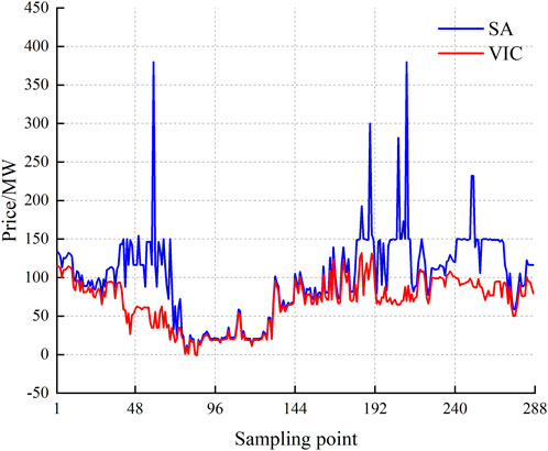
Figure 7 shows the electricity prices for 288 sampling points in the SA and VIC regions in the Australian electricity market for 1 day. The SA regional electricity price fluctuates considerably compared with the VIC regional electricity price, reflecting the spatial variation in electricity prices. The influence of regional electricity price differences is apparent. Therefore, considering the spatial characteristics of regional electricity prices can better mine regional electricity price information.

FIGURE 7

FIGURE 7. Electricity price curve in different regions.

All the data selected from the data set were divided into training, validation, and test sets according to a 7:1:2 ratio (Wang et al., 2021b). The three data sets are normalized by the mean value and standard deviation of the training set:

$\widehat{x}=\frac{x-mean\left(X_{train}\right)}{std\left(X_{train}\right)}(9)$

where x is the initial regional electricity price, $\widehat{x}$ is normalized x, $mean\left(X_{train}\right)$ is the average of the training set, and $std\left(X_{train}\right)$ is the standard deviation of the training set. This paper sets H = 12 and uses the historical data of the last 12 steps to forecast the regional electricity price of the next 12 steps, $T_{out}$ = 12.

4.2 Model parameters and evaluation indicators

The adaptive spatiotemporal prediction framework stacks eight spatiotemporal layers through the jump connection mechanism. The void factor d is sequentially set to (1,2,1,2,2,1,2,2). The size of nodes embedding $E_1$ and $E_2$ are set to 10, and $E_1$ and $E_2$ are initialized randomly. The diffusion step k of Eq. 7 is set to 2, the dropout is set to 0.3, the learning rate is 0.001, the batch size is 64, and the number of iterations is 100.

The average absolute error $I_{\mathrm{M}\mathrm{A}\mathrm{E}}$ and root mean square error $I_{\mathrm{R}\mathrm{M}\mathrm{S}\mathrm{E}}$ are used to compare the predictions of different methods. $I_{\mathrm{M}\mathrm{A}\mathrm{E}}$ and $I_{\mathrm{R}\mathrm{M}\mathrm{S}\mathrm{E}}$ are calculated as follows:

$I_{\mathrm{M}\mathrm{A}\mathrm{E}}=\frac{1}{H_b}{\displaystyle \sum _{m=1}^{H_b}}\left|{\widehat{y}}_m-y_m\right|(10)$

$I_{\mathrm{R}\mathrm{M}\mathrm{S}\mathrm{E}}=\sqrt{\frac{1}{H_b}{\displaystyle \sum _{m=1}^{H_b}}{\left({\widehat{y}}_m-y_m\right)}^2}(11)$

where $y_m$ is the actual value of the mth time step, ${\widehat{y}}_m$ is the predicted value of the mth time step, and $H_b$ is the total number of data sampling points in the test set.

4.3 Example results

This paper compares three different spatial–temporal convolutional networks: the spatial–temporal convolutional network (STGCN), the adaptive spatial–temporal convolutional network (Ada-STGCN), and the non-adaptive spatial–temporal convolutional network (TCN). The spatial–temporal convolutional network contains an adjacency matrix and a learnable adjacency matrix for the geographic information of the five Australian electricity market regions. The adaptive spatial–temporal convolutional network has only one learnable adjacency matrix, the static non-adjacency matrix of the adaptive spatial–temporal convolutional network, which is an identity matrix., Although non-adaptive spatial-temporal convolutional networks have the same framework as spatial–temporal convolutional networks and adaptive spatial–temporal convolutional networks, they only explore temporal features and do not use graph convolutional layers to explore spatial dependencies. In addition, this paper also compares results with the autoregressive model (AR), long short–term memory (LSTM), diffusion convolutional recurrent neural network (DCRNN), and attention based spatial–temporal graph convolutional network (ASTGCN) algorithms.

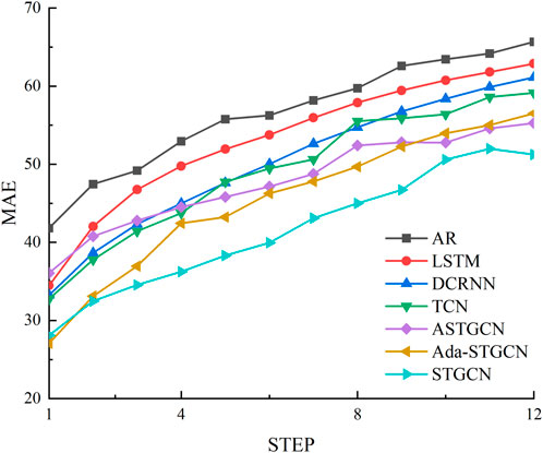
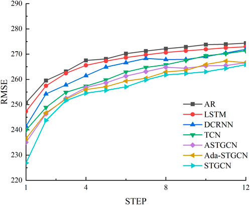
The indicators of the seven models are compared using the algorithm shown in Figure 8 to predict the electricity prices in the five Australian regions. The STGCN is significantly better than the Ada-STGCN and ASTGCN, and the twelve-step STGCN prediction is always better. Compared with the ASTGCN, the STGCN first-step predictions are slightly lower than the Ada-STGCN and are better in the other eleven-step predictions. The Ada-STGCN is better than the ASTGCN in the prediction before nine steps, while the ASTGCN is better than the Ada-STGCN starting from the 10th step, and the ASTGCN is better for longer-step predictions. The non-adaptive spatial–temporal convolutional network is slightly better than the LSTM because the LSTM only mines the temporal dimension information by TCN. Among the seven models, the spatial–temporal convolutional network has the best predictions, and its $I_{\mathrm{M}\mathrm{A}\mathrm{E}}$ is the lowest, with a maximum 22% improvement compared with the ASTGCN, but with the same disadvantages as the ASTGCN. It must provide a connected adjacency matrix, and the input data is complex and difficult to obtain.

FIGURE 8

FIGURE 8. MAE comparison of predictive models.

Figure 9 compares the indicators of the seven models. The trends of the $I_{\mathrm{R}\mathrm{M}\mathrm{S}\mathrm{E}}$ indicators are the same as for the $I_{\mathrm{M}\mathrm{A}\mathrm{E}}$, and the prediction results of the STGCN are better than those of the other six model algorithms. The indicators of the Ada-STGCN and ASTGCN models are similar. Each model has certain advantages.

FIGURE 9

FIGURE 9. RMSE comparison of predictive models.

In Figures 8, 9, the prediction results of the adaptive spatial–temporal convolutional network are always better than those of the non-adaptive spatial–temporal convolutional network. This result shows that the adaptive adjacency matrix can learn the spatial dimension of the regional electricity price. If the adjacency matrix in the spatial–temporal convolutional network is simply a static identity, the spatial dimension features of regional electricity prices cannot be effectively mined. The adaptive spatial–temporal convolutional network prediction framework proposed in this paper has no prior knowledge of the edges between regions. Compared with the STGCN, a certain amount of predictive accuracy is sacrificed, but it has the advantage that the required data is only electricity price historical data, which does not increase the data requirements. The adaptive spatial–temporal convolutional network is a compromise after weighing the predictive accuracy and the difficulty of data acquisition and improves the predictive accuracy to a certain extent without increasing the data requirements. From the evaluation indicators, the Ada-STGCN is better than the ASTGCN and does not require prior edge knowledge.

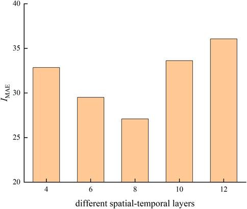
This paper also analyzes the influence on the prediction results when the model parameters are changed. The number of spatial–temporal layers of the adaptive spatial–temporal convolutional network and the k value of the diffusion step noticeably influence the prediction results. The void factor d, node embedding size, dropout value, learning rate, and batch size values used are based on general experience.

From Figure 10, given the influence of different diffusion step k values on the prediction results, the prediction result is best when the diffusion step k is set to 2. The predictive accuracy increases initially and then decreases with increasing diffusion step k. The k value of the diffusion step refers to the influence range between nodes, where k = 1 represents the influence between a node and the adjacent node, k = 2 represents the influence between the node, the adjacent node, and the next adjacent node, and so on when k takes other values. The results in Figure 10 show that the prediction results are best when considering the second-order adjacent regions. Considering only the first-order adjacent regions leads to insufficient exploration. When considering the third and higher orders, uncorrelated regional features become mixed, leading to a decline in predictive accuracy.

FIGURE 10

FIGURE 10. Influence of k value of different diffusion steps on prediction results.

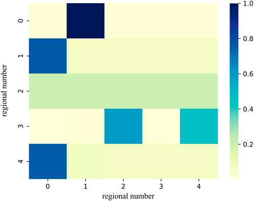
The adaptive adjacency matrix of the spatial–temporal convolutional network is randomly initialized and trained using stochastic gradient descent. The adaptive adjacency matrix changes every spatial–temporal convolutional network cycle and is closely related to its random initialization parameters. Figure 11 is an adaptive adjacency matrix for electricity price prediction of the five Australian regions, reflecting the spatial connectivity relationship between electricity prices in different regions learned for each cycle. The numbers 0–4 in Figure 11 represent the five regions, and each matrix element represents the spatial connectivity relationship between the two regions (ranging from 0 to 1).

FIGURE 11

FIGURE 11. Adaptive adjacency matrix for spatial-temporal convolutional networks.

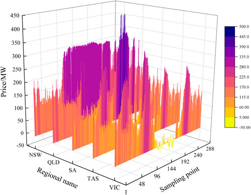
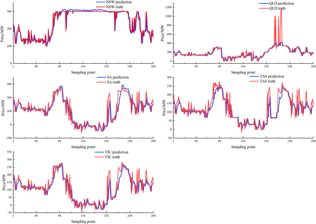
Figure 12 shows the spatial–temporal forecast of electricity prices for the five regions for 288 sampling points over 1 day, indicating spatial differences between regions. The price fluctuation in the QLD region is the largest because the power grid in this region is not connected to the main network. Over many periods, the regional power grid cannot operate at the price of the national electricity market. Power flows between the power grids in different regions may be blocked, leading to regional power price fluctuations, meaning that the power output area market price is low, and the power input area market price is high. These factors impact the spatial distribution of electricity prices. The adaptive spatial–temporal prediction framework proposed in this paper can effectively learn and mine its spatial–temporal dependencies without prior knowledge. Figure 13 shows the predicted and actual values of electricity prices in the five regions for 288 sampling points over the day in Figure 12. The electricity price prediction results for the five regions are very good, indicating that the adaptive spatiotemporal forecasting framework proposed in this paper can effectively excavate the potential spatial dependence of electricity prices in different regions.

FIGURE 12

FIGURE 12. Spatial-temporal forecasting of regional electricity prices.

FIGURE 13

FIGURE 13. Prediction and actual value of regional electricity prices.

5 Conclusion

This paper proposes an electricity price prediction framework based on an adaptive spatial–temporal convolutional network. The study is aimed at large fluctuations in the regional electricity price spot market, forecasting challenges, and difficulty obtaining spatial adjacency information, taking the operational data of the Australian electricity market as an example. The following conclusions are drawn from the analysis of calculations examples:

(1) The prediction framework proposed in this paper, on the basis of mining the time dependence of spot electricity prices, considers the spatial influence of other spot electricity prices, and adopts GCN to mine the spatial dependence of spot electricity prices. In the 12-step forecast of this example, considering the spatial dependence of the spot electricity price can improve the prediction accuracy by at least 10.3% and at most 19.8%. The example results show that mining the spatial dependence of the spot electricity price can help Improve forecast accuracy.

(2) The adaptive adjacency matrix proposed in this paper can solve the problem that GCN cannot be used to mine the spatial dependence of spot electricity prices when the edge prior knowledge is unknown or lacking.

(3) The prediction framework proposed in this paper has further improved prediction accuracy compared with baseline models (AR, LSTM, and TCN) and other similar models (DCRNN, ASTGCN). In the twelve-step prediction, the prediction accuracy of STGCN is up to 32.8% higher than AR, up to 27.2% higher than LSTM, up to 19.8% higher than TCN, up to 20.2% higher than DCRNN, and up to 22.1% higher than ASTGCN.

The adaptive spatial–temporal convolutional network prediction framework in this paper requires the same lengths for the electricity price historical data in all regions. This means that the step size is the same for all nodes, representing a shortcoming of the proposed adaptive spatial–temporal convolutional network prediction framework. Future research will combine this paper’s method with time series decomposition to improve forecast accuracy. We will also study other GNN prediction issues related to applications in the power field.

Data availability statement

Publicly available datasets were analyzed in this study. This data can be found here: https://www.aemo.com.au/energy-systems/electricity/national-electricity-market-nem/data-nem/aggregated-data.

Author contributions

JX: Conceptualization, data curation, writing original draft, writing—review and editing. BH: Funding acquisition, methodology, project administration. PZ: Conceptualization, data curation, writing—original draft, writing—review and editing. XZ: Conceptualization, data curation, funding acquisition, writing—review and editing. ZX: Conceptualization, data curation, writing-original draft, writing—review and editing. ZH: Formal analysis, validation, visualization, writing—review and editing. All authors contributed to the article and approved the submitted version.

Funding

This work was supported by the National Key R&D Program of China (2022YFB4100802), National Natural Science Foundation of China (U1908217 and U22B20115).

Conflict of interest

Author BH was employed by State Grid Dalian Electric Power Supply Company. XZ was employed by State Grid Liaoning Electric Power Co. Ltd.

The remaining authors declare that the research was conducted in the absence of any commercial or financial relationships that could be construed as a potential conflict of interest.

Publisher’s note

All claims expressed in this article are solely those of the authors and do not necessarily represent those of their affiliated organizations, or those of the publisher, the editors and the reviewers. Any product that may be evaluated in this article, or claim that may be made by its manufacturer, is not guaranteed or endorsed by the publisher.

References

Abate, G. D., and Haldrup, N. (2017). Space-time modeling of electricity spot prices. Energy J.38, 175–196. doi:10.5547/01956574.38.5.GABA

CrossRef Full Text | Google Scholar

Afrasiabi, M., Mohammadi, M., Rastegar, M., and Kargarian, A. (2019). Probabilistic deep neural network price forecasting based on residential load and wind speed predictions. Renew. Power Gener. IET13 (11), 1840–1848. doi:10.1049/iet-rpg.2018.6257

CrossRef Full Text | Google Scholar

Atwood, J., and Towsley, D. “Diffusion-convolutional neural networks,” in Proceedings of the Conference and Workshop on Neural Information Processing Systems (NIPS), Barcelona, Spain, 2016, 1993–2001. doi:10.48550/arXiv.1511.02136

CrossRef Full Text | Google Scholar

Chitsaz, H., Zamani-Dehkordi, P., Zareipour, H., and Parikh, P. (2018). Electricity price forecasting for operational scheduling of behind-the-meter storage systems. IEEE Trans. Smart Grid9 (6), 6612–6622. doi:10.1109/TSG.2017.2717282

CrossRef Full Text | Google Scholar

Deng, Z., Liu, C., and Zhu, Z. (2021). Inter-hours rolling scheduling of behind-the-meter storage operating systems using electricity price forecasting based on deep convolutional neural network. Int. J. Electr. Power and Energy Syst.125, 106499. doi:10.1016/j.ijepes.2020.106499

CrossRef Full Text | Google Scholar

Geng, X., Li, Y., Wang, L., Zhang, L., Liu, Y., Ye, J., et al. (2019). Spatiotemporal multi-graph convolution network for ride-hailing demand forecasting. Proc. AAAI Conf. Artif. Intell.33, 3656–3663. doi:10.1609/aaai.v33i01.33013656

CrossRef Full Text | Google Scholar

Goyal, P., and Ferrara, E. (2017). Graph embedding techniques, applications, and performance: A survey. Knowledge-Based Syst.151, 78–94. doi:10.1016/j.knosys.2018.03.022

CrossRef Full Text | Google Scholar

Hafeez, G., Alimgeer, K. S., Wadud, Z., Khan, I., Usman, M., Qazi, A. B., et al. (2020a).An innovative optimization strategy for efficient energy management with day-ahead demand response signal and energy consumption forecasting in smart grid using artificial neural network. IEEE Access8, 84415–84433. doi:10.1109/ACCESS.2020.2989316

CrossRef Full Text | Google Scholar

Hafeez, G., Javaid, N., Riaz, M., Ali, A., Umar, K., and Iqbal, Z. (2020b). Day ahead electric load forecasting by an intelligent hybrid model based on deep learning for smart grid. Adv. Intelligent Syst. Comput.993, 36–49. doi:10.1007/978-3-030-22354-0_4

CrossRef Full Text | Google Scholar

Hafeez, G., Khan, I., Jan, S., Shah, I. A., Khan, F. A., and Derhab, A. (2021). A novel hybrid load forecasting framework with intelligent feature engineering and optimization algorithm in smart grid. Appl. Energy299, 117178. doi:10.1016/j.apenergy.2021.117178

CrossRef Full Text | Google Scholar

Han, S., Hu, F., Chen, Z., Zhang, L., and Bai, X. (2022). Day ahead market marginal price forecasting based on GCN-LSTM. Proc. CSEE42 (9), 3276–3285. doi:10.13334/j.0258-8013.pcsee.202548

CrossRef Full Text | Google Scholar

Jahangir, H., Tayarani, H., Gougheri, S. S., Golkar, M. A., and Elkamel, A. (2021). Deep learning-based forecasting approach in smart grids with microclustering and bidirectional LSTM network. IEEE Trans. Industrial Electron.68 (9), 8298–8309. doi:10.1109/TIE.2020.3009604

CrossRef Full Text | Google Scholar

Jin, L., Liu, W., Wang, X., Yu, J., and Zhao, P. (2021). Analyzing information disclosure in the Chinese electricity market. Front. Energy Res.9, 655006. doi:10.3389/fenrg.2021.655006

CrossRef Full Text | Google Scholar

Lago, J., Ridder, F. D., and Schutter, B. D. (2018). Forecasting spot electricity prices: Deep learning approaches and empirical comparison of traditional algorithms. Appl. Energy221, 386–405. doi:10.1016/j.apenergy.2018.02.069

CrossRef Full Text | Google Scholar

Li, Y., Yu, R., Shahabi, C., and Liu, Y. (2018). Diffusion convolutional recurrent neural network: Data-driven. Traffic Forecast. Int. Conf. Learn. Represent.3, 1–16. doi:10.48550/arXiv.1707.01926

CrossRef Full Text | Google Scholar

Lu, X., Qiu, J., Lei, G., and Zhu, J. (2022). Scenarios modelling for forecasting day-ahead electricity prices: Case studies in Australia. Appl. Energy308, 118296. doi:10.1016/j.apenergy.2021.118296

CrossRef Full Text | Google Scholar

Luo, Y., Zhang, S., Zhou, B., Li, G., Hu, B., Liu, Y., et al. (2022). Multi-time scale trading profit model of pumped storage power plant for electricity market. Front. Energy Res.10, 975319. doi:10.3389/fenrg.2022.975319

CrossRef Full Text | Google Scholar

Niet, I., van Est, R., and Veraart, F. (2021). Governing AI in electricity systems: Reflections on the EU artificial intelligence bill. Front. Artif. Intell.4, 690237. doi:10.3389/frai.2021.690237

PubMed Abstract | CrossRef Full Text | Google Scholar

Portela, J., Munoz, A., and Alonso, E. (2016). Forecasting functional time series with a new hilbertian ARMAX model: Application to electricity price forecasting. IEEE Trans. Power Syst.33 (1), 545–556. doi:10.1109/TPWRS.2017.2700287

CrossRef Full Text | Google Scholar

Qiao, W., and Yang, Z. (2020). Forecast the electricity price of U.S. using a wavelet transform-based hybrid model. Energy193, 116704. doi:10.1016/j.energy.2019.116704

CrossRef Full Text | Google Scholar

Sun, W., Zhu, S., and Yang, J. (2022). Topology identification of microgrid based on graph convolutional network. Automation Electr. Power Syst.46 (5), 71–81. doi:10.7500/AEPS20210531005

CrossRef Full Text | Google Scholar

Tan, Z., Ruan, G., Zhong, H., and Xia, Q. (2018). Security pre-check method of bilateral trading adapted to independence of power exchange. Automation Electr. Power Syst.42 (10), 106–113. doi:10.7500/AEPS20171005002

CrossRef Full Text | Google Scholar

Toubeau, J. F., Morstyn, T., Bottieau, J., Zheng, K., Apostolopoulou, D., Vallee, F., et al. (2021). Capturing spatio-temporal dependencies in the probabilistic forecasting of distribution locational marginal prices. IEEE Trans. Smart Grid12 (3), 2663–2674. doi:10.1109/TSG.2020.3047863

CrossRef Full Text | Google Scholar

Tschora, L., Pierre, E., Plantevit, M., and Robardet, C. (2022). Electricity price forecasting on the day-ahead market using machine learning. Appl. Energy313, 118752. doi:10.1016/j.apenergy.2022.118752

CrossRef Full Text | Google Scholar

Uniejewski, B., Marcjasz, G., and Weron, R. (2017). On the importance of the long-term seasonal component in day-ahead electricity price forecasting: Part II - probabilistic forecasting. Energy Econ.79, 171–182. doi:10.1016/j.eneco.2018.02.007

CrossRef Full Text | Google Scholar

Wan, C., Niu, M., Song, Y., and Xu, Z. (2017). Pareto optimal prediction intervals of electricity price. IEEE Trans. Power Syst.32 (1), 817–819. doi:10.1109/TPWRS.2016.2550867

CrossRef Full Text | Google Scholar

Wang, J., Jiang, J., Jiang, W., Li, C., and Zhao, W. “LibCity: An open library for traffic prediction,” in Proceedings of the 29th International Conference on Advances in Geographic Information Systems, New York, NY, United States, November 2021b, 45–148.

Google Scholar

Wang, Z., Zhou, Y., Guo, Q. Q., and Sun, H. (2021a). Transient stability assessment of power system considering topological change: A message passing neural network-based approach. Proc. CSEE41 (7), 2341–2350. doi:10.13334/j.0258-8013.pcsee.202139

CrossRef Full Text | Google Scholar

Wei, Q., Chen, S., HuanMa, W., and Tao, C. (2021). Forecasting method of clearing price in spot market by random forest regression. J. Chin. Electr. Eng. Sci.41 (4), 1360–1367. doi:10.13334/j.0258-8013.pcsee.191904

CrossRef Full Text | Google Scholar

Wu, Z., Pan, S., Long, G., Jiang, J., and Zhang, C. “Graph wavenet for deep spatial-temporal graph modeling,” in Proceedings of the International Joint Conference on Artificial Intelligence (IJCAI), Macao, China, August 2019, 1907–1913. doi:10.24963/ijcai.2019/264

CrossRef Full Text | Google Scholar

Xiao, C., Sutanto, D., Muttaqi, K. M., Zhang, M., Meng, K., and Dong, Z. (2021). Online sequential extreme learning machine algorithm for better predispatch electricity price forecasting grids. IEEE Trans. Industry Appl.57 (2), 1860–1871. doi:10.1109/TIA.2021.3051105

CrossRef Full Text | Google Scholar

Xu, B., Cen, K., and Huang, J. (2020). A survey on graph convolutional neural network. Chin. J. Comput.43 (5), 755–780. doi:10.11897/SP.J.1016.2020.00755

CrossRef Full Text | Google Scholar

Yang, Y., Liu, J., Xu, X., Xie, K., Lai, Z., Xue, Y., et al. (2022). Cooperative trading strategy of carbon emitting power generation units participating in carbon and electricity markets. Front. Energy Res.10, 977509. doi:10.3389/fenrg.2022.977509

CrossRef Full Text | Google Scholar

Yang, Y., Tan, Z., Yang, H., Ruan, G., Zhong, H., and Liu, F. (2021). Short-term electricity price forecasting based on graph convolution network and attention mechanism. IET Res. Journals16, 2481–2492. doi:10.1049/rpg2.12413

CrossRef Full Text | Google Scholar

Zhang, J., Tan, Z., and Wei, Y. (2020). An adaptive hybrid model for short term electricity price forecasting. Appl. Energy258, 114087. doi:10.1016/j.apenergy.2019.114087

CrossRef Full Text | Google Scholar