Assay data of spent nuclear fuel: the lab-work behind the numbers

Computational modelling for spent nuclear fuel (SNF) characterization is already widely used and continuously further developed for a plethora of safety related applications and licensing issues in SNF management. An essential step in the development of these methodologies is the validation: the demonstration that the SNF elemental and isotopic composition is sufficiently accurately predicted by the code calculations. This validation step requires experimentally measured nuclide concentrations in SNF, together with an estimation of related uncertainties. The SFCOMPO 2.0 database of OECD/NEA is a database of such publicly available assay data of SNF. A basic understanding of all analytical steps that finally result in assay data of SNF is important for modelers when assessing the “fit-for-validation” requirement of an experimental dataset. The aim of this article is to explain users of such datasets the complex analytical pathway towards assay data. Points of attention, challenges and pitfalls all along the analytical pathway will be discussed, from sampling, dissolution procedures, necessary dilutions and separations, available analytical techniques, some related uncertainties, up to reporting of the results.

Introduction

Safe and secure nuclear fuel management requires detailed knowledge of the nuclear fuel composition at all stages of the fuel cycle. This is particularly true for Spent Nuclear Fuel (SNF), the nuclear fuel after discharge from the nuclear reactor in which it was used. Many applications require the detailed composition of SNF as input data, e.g., criticality safety calculations, source term data for accident research, safety assessments of wet and dry storage systems, transportation cask designs, reprocessing schemes, and geological repository safety analyses. Destructive chemical analysis can provide the more detailed composition of SNF samples. Non-destructive analyses (NDA) can also provide valuable composition data, however, NDA is a completely different domain and out of the scope of this article.

SNF analyses are challenging because of the high dose-rate of the samples. The first part of the sample preparation can only be performed in hot-cells. Only after further dilutions and/or separations, the dose-rate will be low enough for further sample handling in glove boxes and/or fume hoods. Depending on the nature and dose-rate of the ready-to-measure samples, the analytical instruments might need ‘nuclearization’ for the analysis of SNF samples. An example of such ‘nuclearized’ system is a mass spectrometer of which the sample introduction system is installed in a glove box for safe sample handling. These specificities of SNF analyses make them very demanding, time-consuming and expensive. Computational modelling of SNF characterization is an interesting alternative methodology. An essential step in the development of these methodologies is the validation: the demonstration that the SNF elemental and isotopic composition is sufficiently accurately predicted by the code calculations. This validation step requires experimentally measured nuclide concentrations in SNF, together with an estimation of related uncertainties.

Many experimental SNF analysis programs (Nodvik, 1966; Nodvik, 1969; Atkin, 1981; Davis and Pasupathi, 1981; Bierman and Talbert, 1994; Guenther et al, 1994; Belgonucléaire, 2000; Brady-Raap and Talbert, 2001; Baeten et al, 2003; Shinohara et al, 2003; Boulanger et al, 2004; Zwicky et al, 2004; Conde et al, 2006; Markova et al, 2006; Yamamoto and Kawashima, 2007; Makarova et al, 2008; Zwicky, 2008; Alejano et al, 2009; Zwicky et al, 2010; Govers et al, 2015) have been organized, aiming at new datasets of nuclide concentrations for, e.g., code validation. Most of these datasets remain confidential for a certain time, only available for the financers of the program. OECD/NEA has a long tradition of collecting the datasets after the confidentiality period, and making them publicly available via the SF-COMPO database (Michel-Sendis et al, 2017). For an experimental dataset of SNF characterization to be useful for code validation, also the detailed irradiation history of the SNF samples needs to be known and is included in the SF-COMPO database.

This article aims at informing the modelers about the complex analytical pathway leading to such experimental data sets of SNF composition, including many challenges and pitfalls. Also for modelers, a basic understanding of all analytical steps is important when assessing the ‘fit-for-validation’ requirement of an experimental dataset. However, this article does not claim for completeness, as many variations are possible. This article can serve as introduction to similar and more extensive descriptions of SNF analyses as published in the past (Wolf et al, 2005; Brennetot and Chartier, 2006; Wachel, 2007; Günther-Leopold et al, 2008; OECD NEA, 2011). These references can be consulted for additional information and further references.

Spent nuclear fuel

Every analytical chemist can confirm: the better you know your sample, the better you can perform your analysis. That is not different for Spent Nuclear Fuel (SNF) and as some of the analytical challenges find their origin in the very nature of SNF, it is worth discussing them upfront. The most used nuclear fuel for modern light-water reactors (LWR) is ceramic UO₂ in the shape of pellets, about 1 cm in height and 1 cm in diameter. The fresh nuclear fuel, before irradiation in a nuclear reactor, is very homogeneous and pure. Quality control of the production guarantees a concentration limit on impurities.

After irradiation in the reactor, the story is completely different as the now spent nuclear fuel became very inhomogeneous with variations in composition depending on a. o. reactor type, irradiation history, (local) burn-up and cooling time. Fission of the fissile nuclides resulted in a multitude of fission products whereas neutron capture by fertile heavy nuclides produced higher actinides. At fuel pin level, there is a longitudinal elemental concentration profile of all these fission and activation products, depending on the local burn-up. At pellet level, there is also a radial elemental concentration profile due to the difference in local burn-up. These concentration profiles also depend on the type of fission product. Kleykamp (Kleykamp, 1985) categorized the fission products in.

• Elements that are soluble in the uranium dioxide matrix, such as the rare earth elements (REE), Zr and Nb

• Inert gases (Xe and Kr) that have a very low solubility in the ceramic matrix and accumulate in gas bubbles

• Metallic precipitates that contain noble metals (Ru, Rh, Tc, Pd) as well as Mo

• Oxide precipitates such as the so-called grey phase (Ba,Sr) (Zr,U,Pu)O₃ or caesium uranates

• Other secondary phases such as CsI

In addition, the huge radial temperature difference between the cooler pellet rim and hotter pellet center affect the local concentration of some fission products. The more volatile species like Cs and I will tend to diffuse to the rim, while elements like Zr and Nb will tend to move to the center. A detailed discussion of fission product behavior in SNF (Olander, 1976; Ballagny et al, 2009; Konings et al, 2010; Spahiu, 2021) is beyond the scope of this article, but these phenomena just illustrate the complexity and inhomogeneity of SNF. It may be clear that already the sampling of such inhomogeneous material like SNF is a crucial step in producing representative SNF composition results by destructive analysis.

Lab work

Sampling

In view of the inhomogeneity of SNF, the sampling strategy for a representative sample for destructive chemical and radiochemical characterization analysis has to be chosen carefully.

It is general practice to perform first a gamma scan of the complete fuel pin to determine the axial variations in activity. Such gamma scan clearly shows the activity profile, with lower activities at bottom and top of the fuel pin and a more stable activity level in the middle part of the fuel pin (corresponding to the more stable neutron densities in the middle part of the reactor during irradiation time). The exact positions of the fuel pellets are also clearly visible in such longitudinal fuel pin scans, which is very helpful in defining the precise segment of the fuel pin to sample for destructive analysis.

The sample size should be “fit for purpose”. Figure 1 shows the cutting of a slice of SNF in a hot-cell. When aiming for a complete inventory analysis, the inhomogeneity of the SNF has to be taken into account. As mentioned above, part of the more volatile fission products tend to migrate to the cooler outer sides of the fuel pellet and might accumulate in the fuel–cladding gap and the inter-pellet areas. Therefore, a large enough sample should be chosen, including such inter-pellet area when sampling for complete inventory analysis. This is best achieved by cutting from mid-pellet to mid-pellet, including that way a full inter-pellet area. The corresponding equivalent of one full pellet is the minimum sample size for a complete inventory analysis, though two or three pellets (thus including two or three inter-pellet areas) might even be preferred. For the same reason, the SNF sample should not be de-cladded as the fuel-cladding gap, enriched in more volatile fission products, might be disturbed. This risk is less pronounced with lower burn-up fuels, as the fuel-cladding gap might not be closed yet. For non-mobile nuclides, smaller sample sizes can still be adequate.

FIGURE 1

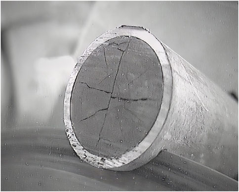
FIGURE 1. cutting a slice of a SNF rod in a hot-cell (remark: this slice is too small for a full inventory analysis of the SNF but it was used for other research purposes).

Dissolution and dilution

The next step along the analytical pathway is the dissolution of the properly weighed SNF sample with its cladding. The cladding is still around the SNF sample not to disturb the fuel-cladding gap where the more volatile and mobile fission products might have moved to. Preferably, the cladding itself will not be dissolved in the dissolution procedure, as that extra (mainly natural) material in the final solution might cause some interferences in later analyses. An example of such interference is the natural Zr-90 interference from dissolved Zircaloy cladding on the fission Sr-90 measurement by mass spectrometry.

The acid of choice in most dissolution procedures for LWR uranium-based fuels is HNO₃ (nitric acid) (Inoue, 1986). HCl (hydrochloric acid), is too corrosive for extensive use in a hot-cell environment. In a first step, the fuel sample + cladding is put in boiling 8–10 M HNO₃ under reflux for several hours. Figure 2 shows such dissolution set-up in a hot-cell. Most of the SNF will have dissolved but the cladding remains undissolved. The cladding will be removed, rinsed, dried and properly weighed. The net SNF sample weight is then calculated by subtracting the weight of the undissolved cladding from the original “sample + cladding” weight. Depending on the amount of remaining residue of undissolved fuel, a second dissolution step can be decided for. Mostly to make sure that all PuO₂ was dissolved. The residue will be filtered off and submitted to a second dissolution step in boiling 8–10 M HNO₃ + 0.1 M HF (hydrofluoric acid) for several hours. Once cooled down and again filtered off, this second solution is added to the first one and together they form the ‘mother or stock solution’ of the dissolved SNF.

FIGURE 2

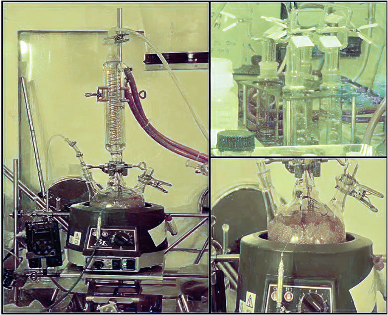
FIGURE 2. Dissolution set-up in a hot-cell: boiling nitric acid under reflux; top right: alkaline wash-bottles to neutralize the acid off-gases and eventually trap the volatile iodine.

There exist slight variations on this dissolution scheme, mainly in terms of molarity of the nitric acid solution and time of heating (Desigan et al, 2019; Momotov et al, 2022). Anyhow, the solubility of SNF has much improved over time as new fabrication methods were developed, specifically for better solubility of SNF in view of later reprocessing schemes. Most modern LWR fuels do not need a two-step procedure anymore to dissolve >99.5% of its U and Pu, but older fuels, especially those with higher Pu-content, remain often a challenge to dissolve completely.

Whether a one-step or a two-step acid dissolution is applied, some residue will anyhow remain (Momotov et al, 2022). The amount of residue varies and depends a. o. on the type of fuel, burnup and dissolution procedure. Typical amounts of residue vary between <0.2% and 2% of the initial SNF amount to be dissolved (Günther-Leopold et al, 2008; Momotov et al, 2022). The residues consist mainly of the so-called ε-particles, metallic precipitates that contain noble metals (Ru, Rh, Tc, Pd) as well as Mo, Ag and Sb. For a complete inventory analysis, these residues will need an extra dissolution step. This can be in a closed bomb system using a combination of concentrated acids or a fusion procedure in molten salts (Wolf et al, 2005; Brennetot and Chartier, 2006; Wachel, 2007; Momotov et al, 2022).

When iodine is also an element of interest for the analysis, special precautions have to be taken at the dissolution step. Iodine in acidic media will form iodine gas and escapes with the off-gases during dissolution. By leading the acidic off-gases through a series of wash-bottles filled with alkaline solution (e.g., 4 M NaOH), the iodine can be trapped (Günther-Leopold et al, 2008). In order to make during dissolution the carry-over of fission iodine to the trapping solution a quantitative process, it is advisable to add a known amount of natural iodine carrier (e.g., KI or NaI) in the dissolution flask.

The whole sampling and dissolution process is hot-cell work. Working clean, not spilling any material, not contaminating any sample, weighing properly in the under-pressure conditions with considerable air-flow of the ventilation system, these are all (daily) challenges for the specialized hot-cell operator.

The stock solution(s) of successfully dissolved SNF are properly weighed and kept under weight control. As the analysis of a complete inventory often takes weeks/months, regularly some further samples or subsamples are needed for the consecutive analysis of all nuclides of interest. Each time a new sample is taken, the stock solution is properly weighed before and after the sample taking so that possible evaporation losses can be checked and corrected for.

To bring dissolved sample material out of the hot-cell for all further analyses, the stock solution will need to be diluted to a level where the dose-rate is low enough to handle in glove boxes. The dilution level needed depends of course of the dose-rate of the stock solution, which reflects the SNF material and amount dissolved, irradiation history and cooling time.

Analyses

A plethora of analytical techniques is available for a detailed characterization of SNF. The best-suited technique depends of course of the nuclide of interest and the envisaged uncertainty level of the final results. E.g., Table 1 resumes the recommended techniques for the actinides. Similar information for relevant fission products can be found in literature (OECD NEA, 2011). However also economical aspects influence the choice. Unfortunately, the costs of an analysis will rather raise exponentially and not linearly, the lower the envisaged uncertainty is.

TABLE 1

TABLE 1. Recommended techniques for actinides and main safety-related spent fuel applications (OECD NEA, 2011).

The most used analytical techniques can be classified in two different groups. At the one hand, there are the radiometric techniques, measuring the decay processes in the SNF by alpha-, beta- and gamma-spectrometry. Neutron emitting nuclides can eventually be measured by neutron-coincidence counting. At the other hand, different mass spectrometry (MS) techniques are often reference techniques for the determination of isotopic vectors and concentrations of elements of interest. These elements of interest may include radionuclides and/or stable nuclides, as both can be measured by MS.

Many of the above-mentioned analytical techniques will need a preliminary separation method, whenever radiometric or isobaric interferences hamper the proper analysis of the nuclide of interest. E.g., separating off the high active Cs before applying gamma spectrometry will decrease the background allowing better gamma analyses of low-energy radionuclides. In MS, typical interference problems in SNF analysis are Pu-238/U-238, Pu-241/Am-241, Pu-242/Cm-242, Pu-244/Cm-244, Nd-148/Sm-148, Nd-150/Sm-150, Nd-144/Ce-144, Sr-90/Zr-90, just to name a few of them.

Separation

Basically, there are two approaches to separations: off-line and on-line. In off-line separations, the separation process is independent from the analytical measurement process. Different fractions of the separation process are collected and the purest ones selected for later analysis. Pure fractions of the element of interest are later on measured with an appropriate analytical technique for the nuclides of interest. This approach allows for longer measurement times on continuous and more stable signals, which is advantageous for the data statistics. In on-line separations, the separation technique is directly coupled to a measurement technique for immediate analysis. This is a much faster and consequently much cheaper approach but by definition dealing with transient, varying signals. Having to deal with transient signals evidently limits the time for data gathering and results in poorer data statistics. As a consequence, the best possible precision of on-line techniques is by definition worse than the best possible precision after off-line separation. However, most often, the choice for off-line or on-line separation is also an economical one. On-line separation coupled with the analytical measurement is by far cheaper as it is much faster, often combines many nuclides of interest in one run (e.g., all lanthanides separated and analyzed in one run) and produces less waste.

Most off-line separations are performed as sample preparation for subsequent Thermal Ionization Mass Spectrometry analysis (TIMS; see description further on) as this analytical technique requires pure elemental fractions for analysis. Most on-line separations (e.g., with Ion Chromatography (IC) or High Performance Liquid Chromatography (HPLC)) are coupled to Inductively Coupled Plasma–Mass Spectrometry (ICP-MS) as ‘detector’ after the separation (e.g., seeFigure 3). It is also common practice in SNF analyses to perform first an off-line separation of the most important matrix elements, U and Pu. Further analyses, eventually including separations, of minor actinides and fission products are then performed on the U- and Pu-free fraction. This eliminates possible matrix effects in later separations and analyses.

FIGURE 3

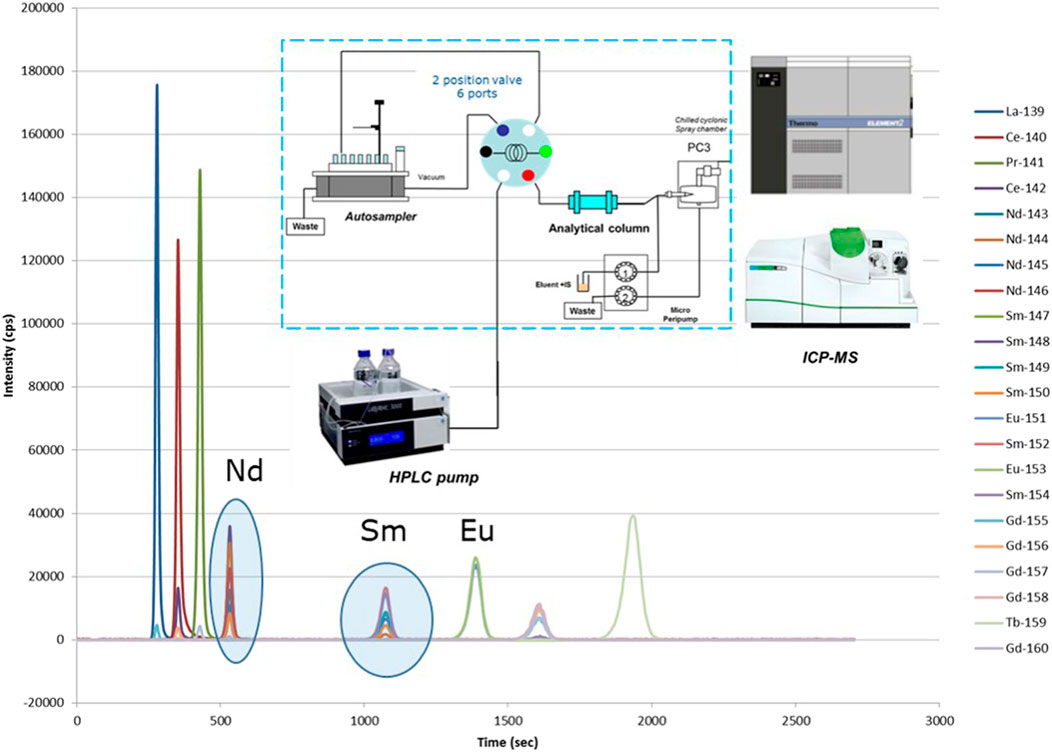
FIGURE 3. Online separation of the lanthanides by HPLC coupled to ICP-MS. Remark: burnup indicator Nd-148 is clearly separated from its isobaric interference Sm-148.

Besides the purity of the separated fractions, another important aspect when discussing separations is whether they need to be quantitative or at least quantified as well. That depends on the analytical technique and calibration used later on. Whenever isotopic dilution is used (see discussion later on), only the purity of the separation is important and not the separation yield (as long as enough material is gathered for the analysis). As isotopic dilution is based on the measurement of isotopic ratios, this calibration technique is insensitive to the separation yield. The isotopic ratios in the pure separated fraction remain the same, independent of the separation yield. Only the counting statistics might be influenced if too little amount of material is gathered after separation. However, when isotopic dilution cannot be used, the separation yield must be determined in order to make a quantitative analysis, e.g., by using tracers. The uncertainty of the separation yield must be taken along when determining the complete experimental uncertainty of the SNF characterization analysis.

Detailed technical information for different separations as applied in SNF characterization analyses can be found in open literature (Röllin et al, 1996; Betti, 1997; Morgenstern et al, 2002; Perna et al, 2002; Todd et al, 2002; Wolf et al, 2005; Brennetot and Chartier, 2006; Isnard et al, 2006; Wachel, 2007; Günther-Leopold et al, 2008; OECD NEA, 2011; Martelat et al, 2018; Trojanowicz et al, 2018; Lin et al, 2020; Wanna et al, 2020; Wanna et al, 2021).

Analysis by radiometric techniques

It is kind of logic that for radioactive nuclides, radiometric analysis techniques are a first option to look at. Depending on the decay mode of the nuclide, the technique of choice can be alpha-spectrometry, liquid scintillation counting (for pure beta-emitters) or gamma-spectrometry.

Alpha-spectrometry can give valuable information about the alpha-emitting nuclides in the SNF solution. In practice (some of the) actinides can be readily analyzed this way. The sample preparation is the most cumbersome step. Only tiny amounts of diluted SNF solution must be loaded on a clean carrier in well-defined way to assure a well-controlled and reproducible geometry. Due to the nature of alpha radiation, self-absorption is a possible issue whenever the sample loading has not been properly made. Alpha-spectrometry of the actinides show discrete peaks according to the energy of the alpha-particle. For quantitative analysis, first the total alpha activity is being measured on a diluted SNF sample. Eventually, different dilutions are being measured of which the results should confirm each other when self-absorption does not play a significant role. The alpha-spectrometry will provide the information how to divide the total activity results over the alpha-emitting nuclides. Unfortunately, some peaks in the alpha-spectrum will be sum-peaks as the energy of the alpha-particles is too close to each other to be separated in the spectrum. In such cases, other techniques will be needed to resolve the interference. A typical example in SNF analysis is the alpha sum-peak of Pu-238 and Am-241. As Am-241 can also be measured by gamma-spectrometry, that gamma result can be used to resolve the interference in alpha-spectrometry. Alternatively, elemental separations can clarify such interferences, as long as the two interfering nuclides are from different elements. The overall measurement uncertainty of alpha-spectrometry is 2% or more at a 95% confidence interval, with as main contributors the sample preparation, the counting statistics and the standard used for calibration (OECD NEA, 2011). Mass spectrometry (MS) is the other technique of choice for the analysis of the actinides in SNF solutions. As the performances of MS (and the required separations) improved a lot over the recent decades, it became the preferred technique for the analysis of actinides in many analytical labs.

Some radionuclides are pure beta-emitters. As beta particles do not have discrete energies, any measurement of beta-activity can only be linked to the nuclide of interest when it has been purified before. Only when measuring pure fractions of the pure beta-emitter, including careful tracking the separation yield, a quantitative analysis is possible. This is a very challenging task when dealing with very radioactive SNF solutions, in which the activity of the pure beta-emitters is overwhelmed by a multitude of gamma- and alpha-emitters. After careful separation, the purified beta-emitter solution is mixed with a commercially available scintillation cocktail. The scintillating organic molecules in the mixture will be excited by the beta-particles from the beta-decay. When going from the excited state back to the ground state, these molecules emit that energy as a photon which can be measured by a photomultiplier. The efficiency of this measurement process needs also to be determined for a quantitative end-result of the analysis. In practice, liquid scintillation counting (LSC) of pure beta-emitters is such a specialized and time-consuming technique that applications in SNF analyses are limited. The overall measurement uncertainty of LSC for a moderately active sample (good counting statistics) is 2% or more at a 95% confidence interval (OECD NEA, 2011). Thanks to the improved sensitivity and selectivity of more recent MS instrumentation, MS became the technique of choice for most beta-emitters as well. Examples of pure beta-emitters of interest in SNF analysis are, e.g., Sr-90, Se-79, …

Gamma-spectrometry remains a very well-established and readily available technique for the analysis of many radionuclides. There are different types of detectors available, each one with its advantages and disadvantages. The best results are relying on semi-conductor technology as developed in high-purity Ge-detectors. The detectors require a careful energy and efficiency calibration. This is readily performed with commercially available calibration solutions, containing certified amounts of gamma-emitting nuclides nicely spread over the energy spectrum. Another important aspect in gamma-spectrometry is the geometry in which calibration standards and samples are measured. As measurement efficiency depends on the geometry of the set-up, this geometry is kept the same for standards and samples. Excellent software help a lot with the interpretation of the gamma-spectra. Figure 4 shows a gamma-spectrum of a SNF. In practice, gamma-spectrometry can be used all along the analytical pathway of SNF solutions: first as orienting analysis technique, based on the most radioactive nuclides in the solution, later for the measurement of specific nuclides in non-separated and/or separated solutions. Cs-137 and Cs-134 nuclides are most often dominating the gamma-spectrum of SNF solutions. The high background this creates on the lower energy side of the spectrum often complicates the analysis of low-energy gamma-emitting nuclides like, e.g., Am-241. A Cs separation can improve significantly the determination of such lower-energy gamma emitting nuclides (Todd et al, 2002; Lin et al, 2020). Many tracers, added to quantify separation yields, are gamma-emitters as their measurement is rather straightforward. The overall uncertainty of a gamma measurement is 3% or more at a 95% confidence interval, with as main contributors the uncertainty of the standard used for efficiency calibration, the counting statistics and to a lesser extent the sample preparation (OECD NEA, 2011). Many of the gamma-emitting nuclides can also be measured by MS. The longer the half-life of the gamma-emitter, the more MS becomes the better choice in terms of sensitivity and achievable uncertainty. Whereas 2 decades ago, as a rule of thumb, MS was the better choice when the half-life of the gamma-emitter was longer than ∼1000 years, this has now become even shorter as the sensitivity of MS improved.

FIGURE 4

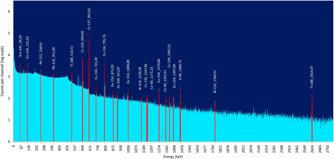
FIGURE 4. Gamma spectrum of SNF from a High Temperature Reactor.

Analysis by mass spectrometry

In SNF analyses, inorganic mass spectrometry (MS), in whatever of its many appearances, is a reference technique. Its success is related to the information it provides: detailed isotopic information for the analyzed elements. The application range is broader, compared to the radiometric analysis techniques, as it is not limited to the radioactive nuclides. The principle of inorganic MS is based on the atomization and ionization of the elements, the separation of the charged atoms (or molecules) in an electrical and/or magnetic field followed by a detector to measure the separated ions. Different mass-spectrometric techniques use different ionization mechanisms, different mass analyzers and different detectors. The first applications of MS in SNF analysis were for the analysis of the long-lived actinides. Nowadays, also many fission products are being analyzed by MS. The most used inorganic MS techniques in SNF analysis are Thermal Ionization Mass Spectrometry (TIMS) and Inductively Coupled Plasma–Mass Spectrometry (ICP-MS).

TIMS

TIMS is a mono-elemental analysis technique for highly purified samples, requiring careful separations in the sample preparation. The analysis is based on the measurement of isotope ratios. As the name already reveals, the ionization mechanism in TIMS is based on heating. A tiny amount (µg-level) of liquid sample is carefully put on a ribbon filament and dried. In the vacuum of the ionization chamber of the instrument, an electrical current heats up the filament to a few hundred degrees and the sample is evaporated, atomized and ionized. Instrumental conditions will differ according to the element to be analyzed. The ions are accelerated and focused into an ion beam. In the magnetic field of a magnetic sector, the ions are separated according to their mass-to-charge ratio. The most used detector for the ions after the mass analyzers is the Faraday cup. In mono-detector instruments, the accelerating voltage and/or magnetic field must be changed for each separated mass-to-charge ratio in order to reach the detector. However, most TIMS instruments are multi-collector instruments, having multiple Faraday cups for measuring simultaneously all isotopes of the element being measured. Simultaneous measurement of all isotopes of an element is very beneficial when measuring isotopic ratios as all signal variations are accounted for. All Faraday cups of a multi-collector instrument need to be calibrated so that (generally small) differences in sensitivity between different Faraday cups can be corrected for.

TIMS instruments are expensive, requiring good maintenance, and sample preparation is tedious and time-consuming. However, TIMS measurements, more specifically when using Isotopic Dilution as quantification method (see calibration methods below), remain a reference technique with excellent precision and accuracy for isotopic measurements of the actinides and (some) fission products in SNF. Measurement uncertainties can be as low as 0.1%–0.5%. Multi-collector ICP-MS instruments nowadays challenge this TIMS status as the reference technique for isotopic measurements.

ICP-MS

ICP-MS is a relatively young technique, with the first instruments becoming commercially available in 1983. The ionization source is an inductively coupled plasma (ICP), well-known from ICP - Optical Emission Spectrometry. In its standard configuration, a liquid sample is sent as aerosol within an Ar gas stream, through a hot ICP (∼7000 K). In the plasma, most elements are ionized with an efficiency of >90%. The fact that ICP is an ionization source at atmospheric pressure makes it unique in the MS field, as all other standard MS techniques have an ionization source already under vacuum. This unique feature allows ICP-MS to be combined online with a wide choice of sample preparation and/or separation techniques like, e.g., ion chromatography, high performance liquid chromatography, direct injection techniques, capillary electrophorese, laser ablation, electro-thermal vaporization and others.

MS requires a high vacuum. This transition from atmospheric pressure to high vacuum goes in two steps. The ions of the ICP first travel through the small orifice of a topped-off cone, the sampler, into an intermediate vacuum. Passing through a second small orifice of a second topped-off cone, the skimmer, brings the ions into the high vacuum of the mass analyzer section. An extraction lens at high negative voltage collects the positive ions and leads them through a set of ion lenses to form an ion beam.

Nowadays there are different types of ICP-MS instruments commercially available on the market (see Figure 5). The first mass analyzers used for ICP-MS were quadrupoles. A quadrupole mass analyzer acts as a mass filter: only one mass-to-charge ratio can follow a stable path through the electrical and magnetic field of the quadrupole before reaching the detector. The quadrupole parameters can be changed very rapidly thus allowing fast scanning of the complete mass range. This fast scanning speed is a major advantage with a rather noisy ionization source like an ICP and when transient signals (e.g., after online separation) are being measured. Quadrupole technologies further developed and nowadays instruments are often equipped with Reaction and/or Collision Cells to cope with isobaric and/or polyatomic interferences. Triple MS instruments are another variant in this type of technologies.

FIGURE 5

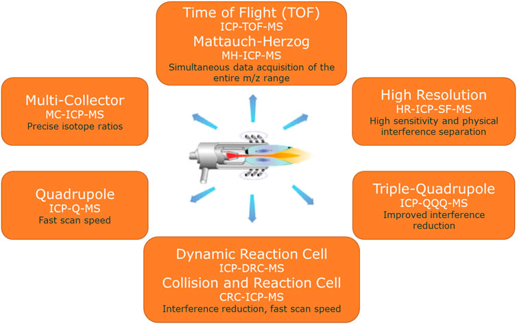
FIGURE 5. Overview of the most prominent ICP-MS instruments with their main characteristic(s).

Another class of mass analyzers used in combination with ICP are the Sector Field (SF) instruments (with a magnetic and an electrical sector). Behind the ion optics, the magnetic sector field focuses the ions with diverging angles of motion from the entrance slit to the intermediate (beta) slit. The magnetic sector field is dispersive with respect to ion energy and mass (exactly: momentum [m*v]). The electric sector analyzer (ESA) focuses ions with diverging angles of motion from the beta slit on to the exit slit. The electric field is dispersive with respect to ion energy (½m*v²) only. Together, if the energy dispersion of magnet and ESA are equal in magnitude but of opposite direction, magnet and ESA focus both ion angles (first focusing) and ion energies (double focusing), while being dispersive for the mass-to-charge ratio (m/z). This order of fields is called reversed Nier-Johnson geometry and is used in single detector SF-ICP-MS instruments. Unlike quadrupole instruments, Sector Field instruments can be equipped with a Multi-collector (MC) system. MC-ICP-MS instruments have another geometry with first the ESA and then the magnet, for better spatial resolution and stability. In terms of achievable precision and accuracy for isotope ratio measurements, modern MC-ICP-MS instruments now compete with TIMS (Isnard et al, 2009). ICP remains a noisier ionization source compared to thermal ionization, but as it is more powerful, more elements can be analyzed (in a shorter time) by MC-ICP-MS.

Single detector ICP-MS instruments are mostly equipped with a Secondary Electron Multiplier (SEM) as detector, whereas multi-collector instruments have a series of Faraday Cups as detectors. SEM detectors are more sensitive, Faraday cups are more robust and stable. Also instruments with the combination of both technologies are available on the market. One additional Faraday Cup in a SEM instrument enlarges the dynamic range of the instrument whereby the instrument automatically switches to the Faraday Cup for the higher concentrations. One SEM in a multi-collector instrument gives the possibility of measuring the lowest abundant isotope with the more sensitive SEM and provides the possibility of scanning a mass range.

The major drawbacks of ICP-MS technology is that it suffers from isobaric and polyatomic interferences. Different approaches are available to cope with these interferences. Simply spoken, in Reaction and/or Collision Cell technologies, a reaction gas or collision gas is used to react or collide the interference away. In SF instruments, the mass resolution can be improved by narrowing the slits in the ion beam path. Mainly poly-atomic interferences can be split from the nuclide of interest, providing the mass difference between nuclide and poly-atomic interference is high enough. By using narrower slits, less ions can enter the mass analyzer and the higher resolution is at the expense of sensitivity. Isobaric interferences like U and Pu on mass 238 or Pu and Am on mass 241 cannot be separated by using narrower slits as the mass difference between these isobaric nuclides is too small. Figure 6 illustrates such interferences in the Am-Cm range of an ICP-MS spectrum of a SNF solution.

FIGURE 6

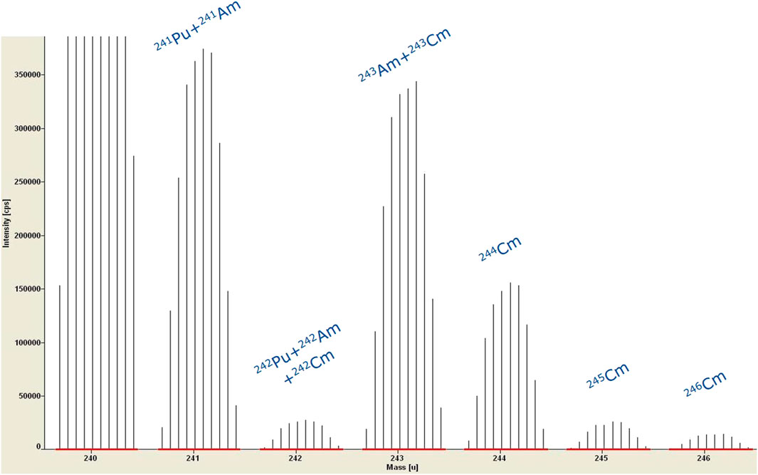
FIGURE 6. ICP-MS spectrum of a SNF solution without any separation; example of isobaric interferences in the Am-Cm range.

In inorganic MS, besides the instrumentation as such (TIMS versus ICP-MS; quadrupole versus sector field MS; single collector versus multi-collector instruments) also the calibration method influences a lot the achievable precision and accuracy. The best precision and accuracy can be reached by using the Isotope Dilution (ID) method on multi-collector instruments (TIMS or MC-ICP-MS). Other calibration methods, mostly for single detector ICP-MS instruments, are external calibration and standard addition.

Isotope dilution mass spectrometry (IDMS)

IDMS (Berglund and De Groot, 2004; Vogl, 2007; Vanhaecke et al, 2009; Vogl and Pritzkow, 2010) is a calibration technique based on isotope ratio measurements (and as such not applicable to mono-isotopic elements). The principle is straightforward at the condition that you have a well-characterized spike of the same element available, being a certified concentration of the element, but with a different certified isotopic composition. By adding a known amount and concentration of such spike with different isotopic composition to a known amount of the sample, a change in isotopic ratios is induced in this blend. Knowing the isotope ratios in the sample (= measured), the isotope ratios in the spike (= certified or measured), the isotope ratios in the blend (= measured), the amount of sample and spike in the blend (= both weighed) and the elemental concentration of the spike (= certified), the elemental concentration in the sample can be calculated. As isotope ratios can be measured with high precision and this ID method is only based on measurements of isotope ratios, the concentration in the sample can be measured with high precision and accuracy.

Just because IDMS is based only on the measurement of isotope ratios and amount weightings, it is such a powerful method. Once the spike is added to your sample and well equilibrated, possible losses of some material due to evaporation or spilling, or small dilution errors do not influence the quality of the end result anymore as the isotope ratios remain unaffected. Separation yields do not need to be known, as they do not affect the isotope ratios either. The purity of the separated fraction is important to avoid isobaric interferences. Systematic errors should be corrected for (e.g., mass discrimination or fractionation effects, detector dead time, … ). As correctly stated by Vanhaecke et al (Vanhaecke et al, 2009): “Finally, ID has the potential to provide very accurate and precise results. It should however be stressed that the use of ID does not guarantee analysis results to be very accurate and precise. If ultimate accuracy and precision are aimed at, then all steps have to be executed with great care and a complete elimination of all sources of systematic error and minimization of all sources of uncertainty have to be aimed at.” The state-of-the-art report (OECD NEA, 2011) of the Nuclear Energy Agency (2011) reports for the analysis of the U-238 concentration in solution by simple ID using U-235 as spike and off-line separation, an uncertainty of better than 0.5% when using MC-ICP-MS and TIMS and better than 2%–3% when using (single detector) quadrupole ICP-MS.

External calibration

For many nuclides, external calibration is the most straightforward approach to come to quantitative results. Especially when the nuclide of interest does not suffer from any isobaric interference. By measuring a series of standards with different concentration, a calibration curve can be established, showing the relation between concentration (= known concentration from the standard solutions) and measurement intensity (mostly expressed as net counts per second). The calibration range should cover the concentration range as expected in the sample. By measuring the intensity of an unknown sample, the calibration curve will tell to which concentration it corresponds. The measurement uncertainty of the end-result depends on the quality of the calibration curve, the intensity of the unknown sample and the position of the unknown sample on the calibration curve. The measurement uncertainty when using external calibration is at its best a few percent.

Standard addition

When the nuclide of interest is free from any isobaric interference but the sample matrix might influence the measurement intensity (e.g., in spent fuel analyses, the high U-concentration might suppress the intensities of other lower concentration nuclides), then ‘standard addition’ is a better choice for calibration. Besides the unknown sample, three to four ‘standards’ are measured in which different amounts of known concentration are added to the unknown sample. A calibration curve can be calculated, this time with the ‘added concentrations’ on the x-axis and the measured (net) intensities on the y-axis. The linear curve will pass through the y-axis at the measured (net) intensity of the unknown sample without any standard addition. The absolute value of the intercept corresponds to the concentration in the unknown sample. The measurement uncertainty when using standard addition is at its best also a few percent, like for external calibration. However, this approach avoids possible systematic errors in case (rotational) matrix effects might cause problems (Ellisson and Thompson, 2008). As different standard concentrations need to be added to each sample, standard addition is a more time-consuming calibration.

Reporting

Nuclear data

Due to the radioactive nature of the samples, assay data always have a reference date linked to the results. The original measurement results most often refer to the day of the measurement. Besides the measurement date as reference date, results are also calculated for one common date for the whole set of measurement results. Most commonly used is the End-Of-Life (EOL) date, the day that the irradiation of the nuclear fuel ended. All decay and in-growth calculations for the timespan between measurement date and EOL reference date make use of nuclear data. For consistency, users of the assay data should check whether their set of nuclear data correspond to the nuclear data used for the EOL calculations as different libraries may contain different nuclear data (Doran et al, 2022). Just to give an example: the half-life of Cm-244 in the ENDF/B-VIII.0 library (18.11 ± 0.03 years) is 0.6% higher than the one in the JEFF3.3 library (18.00 ± 0.10 years). Uncertainty calculations should also include the uncertainties on the nuclear data. Calculations get more complex when off-line separations were made, possibly influencing decay and/or in-growth calculations like, e.g., for Ce-144 and Nd-144, or Pu-241 and Am-241. In such cases, two separate time windows are to be considered: the time in between EOL and the separation date and the time in between separation and measurement dates.

Uncertainties

Analytical measurements always are “best estimates” of the “real value”. How good these estimates (via measurements) are, is expressed in the uncertainty related to the measurement result. The Eurachem/CITAC guide on “Quantifying Uncertainty in Analytical Measurement” (Eurachem/CITAC Guide CG4, 2012) defines the uncertainty (of measurement) as a “parameter associated with the result of a measurement that characterizes the dispersion of the values that could reasonably be attributed to the measurand”.

Each step along the analytical pathway, from sampling up to final result, adds to the total experimental uncertainty. The abovementioned guide (Eurachem/CITAC Guide CG4, 2012) lists typical sources of uncertainty (not necessarily independent!).

• Sampling

• Storage conditions (e.g., contamination; losses over storage time; …)

• Instrument effects (e.g., calibration of analytical balance; memory effects in instruments; …)

• Reagent purity

• Assumed stoichiometry

• Measurement conditions (e.g., humidity; temperature; …)

• Sample effects (e.g., varying recovery; matrix effects; …)

• Computational effects (e.g., selection of calibration model; …)

• Blank correction including uncertainty of the blank

• Operator effects

• Random effects (contribute in all determinations)

The guide stresses the importance of listing all possible sources of uncertainty with proper evaluation of each contribution. This is a tedious and time-consuming task, however, this evaluation effort should not be disproportionate and consider the intended use of the measurement. In practice, this evaluation will help identifying the most important sources of uncertainty. Figure 7 illustrates in a fishbone diagram some typical sources of uncertainty in SNF analyses. Guidelines and examples of such uncertainty evaluations can be found in literature (Eurachem/CITAC Guide CG4, 2012; JCGM 100:2008, 2008; Gluschke et al., 2005; Peters et al, 2011), although this remains a case-by-case effort, which has to be repeated for each analytical procedure. Too many parameters and variables play a role (sample specific, lab specific, procedure specific, …) so that “for each procedure the uncertainties have to be re-evaluated and recalculated” (Peters et al, 2011).

FIGURE 7

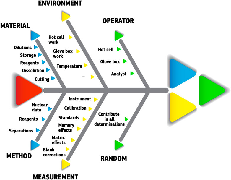
FIGURE 7. Fishbone diagram of some typical contributors to the total experimental uncertainty in SNF analyses. Quantitative data require case-by-case assessment, preferably following internationally accepted guidelines like the “Guide to the expression of uncertainty of measurement” (JCGM 100:2008, 2008) (GUM) or the Eurachem guide “Quantifying uncertainty in analytical measurement” (Eurachem/CITAC Guide CG4, 2012).

Once all sources of uncertainty have been identified and estimated (expressed as standard deviation), all contributions have to be combined into the combined standard uncertainty of the end-result. In assay data, the aim is to have the ‘total experimental uncertainty’ linked to the SNF characterization data. The mathematical correct way of combining all standard uncertainties into a combined standard uncertainty passes via the partial differentials of each component. As such calculations easily get very complicated (for poor chemists like the authors), the guide recommends using a numerical method as developed by Kragten (Kragten, 1994). That method is easily applicable using spreadsheet software. In the Kragten method, the biggest contributors to the combined uncertainty are clearly recognizable. This is very useful during method development, as it shows where most improvements can be made.

The “Guide to the expression of uncertainty in measurement” (JCGM 100:2008, 2008) (also known as ‘the GUM’) correctly states: ‘The evaluation of uncertainty is neither a routine task nor a purely mathematical one; it depends on detailed knowledge of the nature of the measurand and of the measurement procedure’.

The above-described procedure of defining all sources of uncertainty, quantifying them and finally calculating the combined uncertainty, is one way of expressing uncertainty of an analytical measurement. An alternative to this bottom-up approach is the (completely opposite) top-down approach (Maroto et al, 1999; EUROLAB, 2007). In its extreme version, the reproducibility standard deviation, describing the spread of results from the complete analytical procedure in different laboratories, is taken as uncertainty of that analytical procedure. The idea behind this approach is that there will always be unknown sources of uncertainty which then remain unaccounted for and lead to an underestimation of the real uncertainty of the analytical procedure. A detailed discussion on this polarizing topic is out of the scope of this article. However, as inter-laboratory tests for SNF characterization do not exist (and can only be dreamed of) due to the complexity and costs of such an endeavor, only the above-described bottom-up approach can be used to define the uncertainty on SNF analytical results.

It is also worth mentioning that in general, despite all efforts in defining, estimating, calculating measurement uncertainties, existing inter-laboratory studies still show a higher spread in results than can be expected based on the declared measurement uncertainties (AMC, 2003; Thompson and Ellison, 2011; Thompson and Ellison, 2012; Pommé, 2016). Apparently, some contributions to uncertainty are overlooked and as these are not visible in the uncertainty budget, it is called ‘dark uncertainty’ (Thompson and Ellison, 2011; Thompson and Ellison, 2012). There is no easy way out of this discussion. The simplest approach is to raise the coverage factor as suggested in AMC Technical Brief No. 15 ‘Is my uncertainty estimate realistic’ (AMC, 2003): “in cases where information on random and other effects is sparse, rounding k up to 3 instead of using a factor k = 2 is eminently justified on the grounds that the effective degrees of freedom are genuinely low and k = 2 provides inadequate coverage.”

In assay data on SNF with the respective listed uncertainties, it is not always clearly stated what exactly the reported uncertainties represent: is it only the ‘measurement uncertainty’ or is it indeed the ‘total experimental uncertainty’ for the complete analytical pathway. Tracing back the data in the original laboratory report of the analytical lab can help clarifying this important and essential information.

It is also worth noting that correlation data are usually not provided and might need additional inquiries with the analytical lab in order to get a view on that aspect of the assay data. It is clear that, e.g., isotopic compositions based on isotope ratio measurements are correlated (Hibbert, 2003; Meija and Mester, 2007), the sum of all abundances being 100%. That correlation also persists in the concentration results. However, correlations between different elements can be more difficult to trace back, depending, e.g., on the fractions in which the different elements have been determined and the complete analytical pathway of all analyses.

Burnup

Burnup is a key parameter for many codes. By definition, the real burnup is not known but there are several approaches to come to a best estimate. The reactor operator gives already a first estimate, based on the irradiation history of the fuel. A burnup value (in % FIMA (Fissions per Initial Metal Atom)) can also be derived from the assay data, but is not an assay data as such. It is only discussed here as analytical labs are often requested to provide a burnup value based on the results of the chemical analyses of the SNF. The burnup based on assay data are regarded as being more reliable compared to the burnup estimation of the operator of the nuclear reactor.

The burnup can be calculated based on different burnup indicators, nuclides for which the fission yield is (almost) independent of the fissile actinide. Nd-148 is the reference burnup indicator for most LWR fuels as its fission yield for U-235 and Pu-239 is almost the same. Also the other Nd-isotopes can be used as burnup indicators, as well as Cs-137. It is important to check how the analytical lab calculated the burnup, as some steps in the calculation are based on approximations which can be refined by the modelers. One critical step in burnup calculations is the determination of the averaged fission yield. Different approaches for the determination of the averaged fission yield exist and recently, Govers et al (Govers et al, 2022) compared and assessed these approaches. To avoid the shortcomings of existing methods, a novel approach was developed, enabling radiochemical labs to calculate the burnup without the need of dedicated core physics calculations. Whatever the burnup result the analytical lab comes up with, modelers are of course free to calculate themselves a burnup based on the chemical assay data. They might model more detailed fuel composition data at any time of the irradiation, resulting in better estimations of the averaged fission yield and better estimation of the burnup and/or use different nuclear data sets for the calculation. It is also good practice to calculate the burnup based on different burnup indicators. Consistency of the burnups based on different burnup indicators gives more confidence to the dataset.

Conclusion

It may be clear that SNF characterization is a long, complex, time- and resources-consuming effort. Many specialized people are involved along the analytical pathway: the hot-cell operator for the cutting and sampling, often another hot-cell operator for the dissolution and dilutions, lab technicians for the different analytical techniques and a manager to keep track of all the data and combine them in a final analytical result+/-uncertainty in a detailed and complete report. As this is a completely different world compared to the modeling and simulation space, only continuous discussion and communication between the different communities can lead to the best understanding of each other’s questions and needs, and finally to the best results.

Data availability statement

The original contributions presented in the study are included in the article/Supplementary material, further inquiries can be directed to the corresponding author.

Author contributions

SVW wrote the first draft of the manuscript. RA-S, DS, LA, and SVW wrote sections of the manuscript. All authors contributed to the article and approved the submitted version.

Conflict of interest

The authors declare that the research was conducted in the absence of any commercial or financial relationships that could be construed as a potential conflict of interest.

Publisher’s note

All claims expressed in this article are solely those of the authors and do not necessarily represent those of their affiliated organizations, or those of the publisher, the editors and the reviewers. Any product that may be evaluated in this article, or claim that may be made by its manufacturer, is not guaranteed or endorsed by the publisher.

Abbreviations

AMC, Analytical Methods Committee, a committee of the Royal Society of Chemistry Analytical Science Community; CITAC, Cooperation on International Traceability in Analytical Chemistry; ENDF/B-VIII, 8th major release of U.S.‘s Evaluated Nuclear Data File (ENDF); EOL, end of life; ESA, electric sector analyzer; Eurachem, a network of organizations in Europe having the objective of establishing a system for the international traceability of chemical measurements and the promotion of good quality practices; FIMA; fissions per initial metal atom; GUM, guide to the expression of uncertainty in measurement; HPLC, high performance liquid chromatography; IC, ion chromatography; ICP, inductively coupled plasma; ICP-MS, inductively coupled plasma—mass spectrometry/spectrometer; ID, isotope dilution; IDMS, isotope dilution mass spectrometry; JEFF3.3, joint evaluated fission and fusion nuclear data library 3.3; LSC, liquid scintillation counting; LWR, light-water reactor; MC, multi-collector; MC-ICP-MS, multi-collector inductively coupled plasma mass spectrometer; MS, mass spectrometry; NDA, non-destructive analysis; NEA, Nuclear Energy Agency; OECD, Organization for Economic Co-operation and Development; REE, rare-earth element; SEM, secondary electron multiplier; SF, sector field; SF-ICP-MS, sector field inductively coupled plasma mass spectrometry; SFCOMPO, the OECD/NEA web-based spent nuclear fuel isotopic database;SNF, spent nuclear fuel; TIMS, thermal ionization mass spectrometry.

References

Alejano, C., Conde, J. M., Quecedo, M., Lloret, M., Gago, J. A., Zuloaga, P., et al. (2009). “PWR and BWR fuel assay data measurements,” in IAEA International Workshop on Advances in Applications of Burnup Credit for Spent Fuel Storage, Transport, Reprocessing, and Disposition, Córdoba, Spain, 27–30 October 2009.

Google Scholar

AMC (2003). Technical Briefs No 15 (Dec 2003): Is my uncertainty estimate realistic?Available at: www.rsc.org/lap/rsccom/amc/amc_index.ht.

Google Scholar

Atkin, S. D. (1981). Destructive examination of 3-cycle LWR fuel rods from Turkey point unit 3 for the climax – spent fuel test. Washington: Hanford Engineering Development Laboratory. HEDL-TME 80-89 (UC-70).

Google Scholar

Baeten, P., D'hondt, P., Sannen, L., Marloye, D., Lance, B., Renard, A., et al. (2003). “The REBUS experimental programme for burn-up credit,” in Proceedings of the 7th International Conference on Nuclear Criticality Safety (ICNC2003), Tokai-mura, Japan, 20–24 October 2003, 645–649. JAERI–Conf 2003–019.

Google Scholar

Ballagny, A., Béchade, J.-L., Bonin, B., Brachet, J.-C., Delpech, M., Dubois, S., et al. (2009). Nuclear fuels, nuclear energy division monograph. Editor Y. Guérin, and J. L. Guillet (France: CEA). CEA/DEN Direction scientifique, CEA Saclay, Gif-sur-Yvette Cedex.

Google Scholar

Belgonucléaire, (2000). “ARIANE international programme final report,”. Report No: AR2000/15 BN Ref 0000253/221 Rev B.

Google Scholar

Berglund, M. (2004). “Introduction to isotope dilution mass spectrometry (IDMS),” in Handbook of stable isotope analytical techniques. Editor P. De Groot (Netherland: Elsevier), 1, 820–834.

CrossRef Full Text | Google Scholar

Betti, M. (1997). Review: Use of ion chromatography for the determination of fission products and actinides in nuclear applications. J. Chromatogr. A789, 369–379. doi:10.1016/s0021-9673(97)00784-x

CrossRef Full Text | Google Scholar

Bierman, S. R., and Talbert, R. J. (1994). Benchmark data for validating irradiated fuel compositions used in criticality calculations. Richland, United States: Pacific Northwest Laboratory. PNL-10045.

Google Scholar

Boulanger, D., Lippens, M., Mertens, L., Basselier, J., and Lance, B. (2004). “High burnup pwr and bwr mox fuel performance: A review of Belgonucléaire recent experimental programs,” in Proceedings of the International Meeting LWR Fuel Performance, Orlando, Florida, September 19–22, 2004 (American Nuclear Society).

Google Scholar

Brady-Raap, M. C., and Talbert, R. J. (2001). Compilation of radiochemical analyses of spent nuclear fuel samples. Richland, United States: Pacific Northwest National Laboratory. PNNL-13677.

Google Scholar

Brennetot, R., and Chartier, F. (2006). “Isotopic and elementary analysis techniques applied to the spent nuclear fuel characterisation,” in The Need for Post-irradiation Experiments to Validate Fuel Depletion Calculation Methodologies: Workshop Proceedings, Prague, Czech Republic, May 2006, 11–12. NEA/NSC/DOC (OECD/NEA, Paris, 2006.31

Google Scholar

Conde, J-M., Alejano, C., and Rey, J-M. (2006). “Nuclear fuel research activities of the consejo de Seguridad nuclear,” in International Conference on LWR Fuel Performance, Salamanca, Spain, October 2006 (Top Fuel).

Google Scholar

Davis, R. B., and Pasupathi, V. (1981). Data summary report for the destructive examination of rods G7, G9, J8, I9, and H6 from Turkey point fuel assembly B17. Washington: Hanford Engineering Development Laboratory. HEDL-TME 80-85 (UC-70).

Google Scholar

Desigan, N., Bhatt, N., Shetty, M. A., Sreekumar, G. K. P., Pandey, N. K., Kamachi Mudali, U., et al. (2019). Dissolution of nuclear materials in aqueous acid solutions. Rev. Chem. Eng.35 (6), 707–734. doi:10.1515/revce-2017-0063

CrossRef Full Text | Google Scholar

Doran, H. R., Cresswell, A. J., Sanderson, D. C. W., and Falcone, G. (2022). Nuclear data evaluation for decay heat analysis of spent nuclear fuel over 1-100 k year timescale. Eur. Phys. J. Plus137, 665. doi:10.1140/epjp/s13360-022-02865-7

CrossRef Full Text | Google Scholar

Ellisson, S. L. R., and Thompson, M. (2008). Standard additions: Myth and reality. Analyst133, 992–997. doi:10.1039/b717660k

PubMed Abstract | CrossRef Full Text | Google Scholar

Eurachem/Citac Guide Cg4, (2012). “The clinical biomist review,” in Quantifying uncertainty in analytical measurement. Editors S. L. R. Ellisson, and A. Williams3 (Europe: Eurachem). Available at: www.eurachem.org.

Google Scholar

EUROLAB (2007). EUROLAB Technical Report 1/2007: Measurement uncertainty revisited: Alternative approaches to uncertainty evaluation. İstanbul, Türkiye: EUROLAB. Available at: https://www.eurolab.org/pubs-techreports.

Google Scholar

Gluschke, M., Wellmitz, J., and Lepom, P. (2005). A case study in the practical estimation of measurement uncertainty. Accred. Qual. Assur.10, 107–111. doi:10.1007/s00769-004-0895-x

CrossRef Full Text | Google Scholar

Govers, K., Adriaensen, L., Dobney, A., Gysemans, M., Cachoir, C., and Verwerft, M. (2022). Evaluation of the irradiation-averaged fission yield for burnup determination in spent fuel assays. EPJ Nucl. Sci. Technol.8, 18. doi:10.1051/epjn/2022018

CrossRef Full Text | Google Scholar

Govers, K., Dobney, A., Gysemans, M., and Verwerft, M. (2015). Technical scope of the REGAL base program, Revision 1.2. Extern. Rep. SCK•CEN-ER-110.

Google Scholar

Guenther, R. J., Blahnik, D. E., and Wildung, N. J. (1994). Radiochemical analyses of several spent fuel approved testing materials. Richland, United States: Pacific Northwest Laboratory. PNL-10113 (UC-802).

Google Scholar

Günther-Leopold, I., Kivel, N., Kobler Waldis, J., and Wernli, B. (2008). Characterization of nuclear fuels by ICP mass-spectrometric techniques. Anal. Bioanal. Chem.390, 503–510. doi:10.1007/s00216-007-1644-x

PubMed Abstract | CrossRef Full Text | Google Scholar

Hibbert, D. B. (2003). The measurement uncertainty of ratios which share uncertainty components in numerator and denominator. Accred. Qual. Assur.8, 195–199. doi:10.1007/s00769-003-0615-y

CrossRef Full Text | Google Scholar

Inoue, A. (1986). Mechanism of the oxidative dissolution of UO₂ in HNO₃ solution. J. Nucl. Mat.138, 152–154. doi:10.1016/0022-3115(86)90271-0

CrossRef Full Text | Google Scholar

Isnard, H., Aubert, M., Blanchet, P., Brennetot, R., Chartier, F., Geertsen, V., et al. (2006). Determination of ⁹⁰Sr/²³⁸U ratio by double isotope dilution inductively coupled plasma mass spectrometer with multiple collection in spent nuclear fuel samples with in situ⁹⁰Sr/⁹⁰Zr separation in a collision-reaction cell. Spectrochim. Acta B61, 150–156. doi:10.1016/j.sab.2005.12.003

CrossRef Full Text | Google Scholar

Isnard, H., Granet, M., Caussignac, C., Ducarme, E., Nonell, A., Tran, B., et al. (2009). Comparison of thermal ionization mass spectrometry and Multiple Collector Inductively Coupled Plasma Mass Spectrometry for cesium isotope ratio measurements. Spectrochim. Acta B64, 1280–1286. doi:10.1016/j.sab.2009.10.004

CrossRef Full Text | Google Scholar

JCGM 100:2008 (2008). Evaluation of measurement data - guide to the expression of uncertainty in measurement, corrected version 2010. available from https://www.bipm.org/en/committees/jc/jcgm/publications.

Google Scholar

Kleykamp, H. (1985). The chemical state of the fission products in oxide fuels. J. Nucl. Mater.131, 221–246. doi:10.1016/0022-3115(85)90460-x

CrossRef Full Text | Google Scholar

Konings, R. J. M., Wiss, T., and Guéneau, C. (2010). “Nuclear fuels,” in The chemistry of the actinide and transactinide elements. Editors L. R. Morss, N. M. Edelstein, and J. Fuger (Dordrecht: Springer). doi:10.1007/978-94-007-0211-0_34

CrossRef Full Text | Google Scholar

Kragten, J. (1994). Tutorial review. Calculating standard deviations and confidence intervals with a universally applicable spreadsheet technique. Analyst119, 2161–2166. doi:10.1039/an9941902161

CrossRef Full Text | Google Scholar

Lin, M., Kajan, I., Schumann, D., Türler, A., and Fankhauser, A. (2020). Selective Cs-removal from highly acidic spent nuclear fuel solutions. Radiochim. Acta108 (8), 615–626. doi:10.1515/ract-2019-3187

CrossRef Full Text | Google Scholar

Makarova, T. P., Bibichev, B. A., and Domkin, V. D. (2008). Destructive analysis of the nuclide composition of spent fuel of WWER-440, WWER-1000, and RBMK-1000 reactors. Radiochemistry50 (4), 414–426. doi:10.1134/s1066362208040152

CrossRef Full Text | Google Scholar

Markova, L., Chrapciak, V., and Chetverikov, A. (2006). “Draft of proposal on VVER-440 PIE supporting BUC methodology, NRI 12 754, rez, Czech republic,” in Also published in The Need for Post-irradiation Experiments to Validate Fuel Depletion Calculation Methodologies: Workshop Proceedings, Prague, Czech Republic, May 2006, 11–12. NEA/NSC/DOC (OECD/NEA, Paris 2006.31

Google Scholar

Maroto, A., Riu, J., Boqué, R., and Rius, F. X. (1999). Estimating uncertainties of analytical results using information from the validation process. Anal. Chim. Acta391, 173–185. doi:10.1016/s0003-2670(99)00111-7

CrossRef Full Text | Google Scholar

Martelat, B., Isnard, H., Vio, L., Dupuis, E., Cornet, T., Nonell, A., et al. (2018). Precise U and Pu isotope ratio measurements in nuclear samples by hyphenating capillary electrophoresis and MC-ICPMS. Anal. Chem.90, 8622–8628. doi:10.1021/acs.analchem.8b01884

PubMed Abstract | CrossRef Full Text | Google Scholar

Meija, J., and Mester, Z. (2007). Signal correlation in isotope ratio measurements with mass spectrometry: Effects on uncertainty propagation. Spectrochim. Acta B62, 1278–1284. doi:10.1016/j.sab.2007.09.005

CrossRef Full Text | Google Scholar

Michel-Sendis, F., Gauld, I., Martinez, J., Alejano, C., Bossant, M., Boulanger, D., et al. (2017). SFCOMPO-2.0: An OECD NEA database of spent nuclear fuel isotopic assays, reactor design specifications, and operating data. Ann. Nucl. Energy110, 779–788. doi:10.1016/j.anucene.2017.07.022

CrossRef Full Text | Google Scholar

Momotov, V. N., Erin, E. A., and Tikhonova, D. E. (2022). Dissolution of spent nuclear fuel samples for analytical purposes. Radiochemistry64 (5), 551–580. doi:10.1134/s1066362222050010

CrossRef Full Text | Google Scholar

Morgenstern, A., Apostolidis, C., Carlos-Marquez, R., Mayer, K., and Molinet, R. (2002). Single-column extraction chromatographic separation of U, Pu, Np and Am. Radiochim. Acta90 (2), 81–85. doi:10.1524/ract.2002.90.2_2002.81

CrossRef Full Text | Google Scholar

Nodvik, R. J. (1966). Evaluation of mass spectrometric and radiochemical analyses of yankee core I spent fuel. Pennsylvania: Westinghouse Electric Corporation - Atomic Power Division. WCAP-6068.

Google Scholar

Nodvik, R. J. (1969). Supplementary report on evaluation of mass spectrometric and radiochemical analyses of yankee core I spent fuel, including isotopes of elements thorium through curium. Pennsylvania: Westinghouse Electric Corporation - Atomic Power Division. TID 4500, WCAP-6086.

Google Scholar

OECD NEA (2011). “Spent nuclear fuel assay data for isotopic validation: State-of-the-art report,”. Report No:NEA/NSC/WPNCS/DOC.5

Google Scholar

Olander, D. R. (1976). Fundamental aspects of nuclear reactor fuel elements. Berkeley, United States: University of California. Technical Report TID-26711-P1. doi:10.2172/7343826

CrossRef Full Text | Google Scholar

Perna, L., Bocci, F., Aldave de las Heras, L., Pablo, J. D., and Betti, M. (2002). Studies on simultaneous separation and determination of lanthanides and actinides by ion chromatography inductively coupled plasma mass spectrometry combined with isotope dilution mass spectrometry. J. Anal. At. Spectrom.17, 1166–1171. doi:10.1039/b202451a

CrossRef Full Text | Google Scholar

Peters, R. J. B., Elbers, I. J. W., Klijnstra, M. D., and Stolker, A. A. M. (2011). Practical estimation of the uncertainty of analytical measurement standards. Accred. Qual. Assur.16, 567–574. doi:10.1007/s00769-011-0829-3

CrossRef Full Text | Google Scholar

Pommé, S. (2016). When the model doesn’t cover reality: Examples from radionuclide metrology. Metrologia53, S55–S64. doi:10.1088/0026-1394/53/2/s55

CrossRef Full Text | Google Scholar

Röllin, S., Kopatjtic, Z., Wernli, B., and Magyar, B. (1996). Determination of lanthanides and actinides in uranium materials by high-performance liquid chromatography with inductively coupled plasma mass spectrometric detection. J. Chromatogr. A739, 139–149. doi:10.1016/0021-9673(96)00037-4

CrossRef Full Text | Google Scholar

Shinohara, N., Nakahara, Y., Kohno, N., and Tsujimoto, K. (2003). “Recent activity on the post-irradiation analysis of nuclear fuels and actinide samples in JAERI,” in Proc. of the 7th Int. Conference on Nuclear Criticality Safety (ICNC2003), Tokai-Ibaraki, Japan, 20-24 October 2003 (Japan Atomic Energy Research Institute). JAERI-Conf 2003-019.

Google Scholar

Spahiu, K. (2021). EURAD state of the knowledge (SoK) report: Spent nuclear fuel. Europe: EURAD. Domain 3.1.1.

Google Scholar

Thompson, M., and Ellison, S. L. R. (2011). Dark uncertainty. Accred. Qual. Assur.16, 483–487. doi:10.1007/s00769-011-0803-0

CrossRef Full Text | Google Scholar

Thompson, M., and Ellison, S. L. R. (2012). Dark uncertainty. Anal. Methods4, 2609–2612. doi:10.1039/c2ay90034c

PubMed Abstract | CrossRef Full Text | Google Scholar

Todd, T. A., Mann, N. R., Tranter, T. J., Šebesta, F., John, J., and Motl, A. (2002). Cesium sorption from concentrated acidic tank wastes using ammonium molybdophosphate-polyacrylonitrile composite sorbents. J. Radioanal. Nucl. Chem.254 (1), 47–52. doi:10.1023/a:1020881212323

CrossRef Full Text | Google Scholar

Trojanowicz, M., Kołacinska, K., and Grate, J. W. (2018). A review of flow analysis methods for determination of radionuclides in nuclear wastes and nuclear reactor coolants. Talanta183, 70–82. doi:10.1016/j.talanta.2018.02.050

PubMed Abstract | CrossRef Full Text | Google Scholar

Vanhaecke, F., Balcaen, L., and Malinovsky, D. (2009). Use of single-collector and multi-collector ICP-mass spectrometry for isotopic analysis. J. Anal. At. Spectrom.24, 863–886. doi:10.1039/b903887f

CrossRef Full Text | Google Scholar

Vogl, J. (2007). Characterisation of reference materials by isotope dilution mass spectrometry. J. Anal. At. Spectrom.22, 475–492. doi:10.1039/b614612k

CrossRef Full Text | Google Scholar

Vogl, J., and Pritzkow, W. (2010). Isotope dilution mass spectrometry - a primary method of measurement and its role for rm certification. MAPAN - J. Metrology Soc. India25 (3), 135–164. doi:10.1007/s12647-010-0017-7

CrossRef Full Text | Google Scholar

Wachel, D. E. S. (2007). Radiochemical analysis methodology for uranium depletion measurements. New York: Knolls Atomic Power Laboratory. KAPL-4859, DOE/LM-06K140.

Google Scholar

Wanna, N. N., Dobney, A., Van Hoecke, K., Vasile, M., and Vanhaecke, F. (2021). Quantification of uranium, plutonium, neodymium and gadolinium for the characterization of spent nuclear fuel using isotope dilution HPIC-SF-ICP-MS. Talanta: HPIC, 221.

Google Scholar

Wanna, N. N., Van Hoecke, K., Dobney, A., Vasile, M., Cardinaels, T., and Vanhaecke, F. (2020). Determination of the lanthanides, uranium and plutonium by means of on-line high-pressure ion chromatography coupled with sector field inductively coupled plasma – mass spectrometry to characterize nuclear samples. J. Chromatogr. A1617, 460839. doi:10.1016/j.chroma.2019.460839

PubMed Abstract | CrossRef Full Text | Google Scholar

Wolf, S. F., Bowers, D. L., and Cunnane, J. C. (2005). Analysis of high burnup spent nuclear fuel by ICP-MS. J. Radioanal. Nucl. Chem.263 (3), 581–586. doi:10.1007/s10967-005-0627-7

CrossRef Full Text | Google Scholar

Yamamoto, T., and Kawashima, K. (2007). “Status of isotopic composition data and benchmark calculation of BWR fuel in Japan,” in Proc. Int. Conf. ICNC2007, St. Petersburg, Russia, 28 May-1 June 2007.

Google Scholar

Zwicky, H-U. (2008). “Isotopic data of sample F3F6 from a rod irradiated in the Swedish boiling water reactor forsmark 3,”. Zwicky Consulting Report No: ZC-08/001.

Google Scholar

Zwicky, H-U., Low, J., Kierkegaard, J., Schrire, D., and Quecedo, M. (2004). “Isotopic analysis of irradiated fuel samples in the Studsvik Hot Cell laboratory”, in International Meeting on LWR Fuel Performance, Orlando, FL, 19–22 September, 2004.

Google Scholar

Zwicky, H-U., Low, J., Granfors, M., Alejano, C., Conde, J., Casado, C., et al. (2010). Nuclide analysis in high burnup fuel samples irradiated in vandellós 2. J. Nucl. Mater.402, 60–73. doi:10.1016/j.jnucmat.2010.04.023

CrossRef Full Text | Google Scholar