Improving solar radiation source efficiency using adaptive dynamic squirrel search optimization algorithm and long short-term memory

Artificial intelligence and machine learning are used to optimize the design parameters of renewable energy sources, which are now regarded as vital components in current clean energy sources. As a result, system requirements can be reduced, and a well-designed system can improve performance. Artificial intelligence approaches in renewable energy sources and system design would significantly cut optimization time while maintaining high modeling accuracy and optimum performance. This study examines machine learning in depth, emphasizing how it can be used in developing renewable energy sources because of the vast range of technologies it can use. This paper approximates the hourly tilted solar irradiation using climate factors. The irradiance is estimated using a hybrid ensemble-learning approach. This approach combines a proposed adaptive dynamic squirrel search optimization algorithm (ADSSOA) with long short-term memory (LSTM) methods. To the best of our knowledge, this combination has not been used for solar radiation. The results are analyzed and contrasted with the outcomes of several recent swarm intelligence algorithms, such as the genetic algorithm, particle swarm optimization, and gray wolf optimizer. The binary ADSSOA approach performed as expected, with an average error of 0.1801 and a standard deviation of 0.0656. The ADSSOA–LSTM model had the lowest root mean square error (0.000388) compared to LSTM’s (0.001221). In addition, the statistical analysis uses 10 iterations of each presented and evaluated method to provide accurate comparisons and reliable results.

1 Introduction

In recent years, the growing demand for energy has led to the exploration of new energy generation methods. One such method is solar energy, which is generated using solar radiation and is used both at home and in commercial settings (Li et al., 2016). However, the amount of solar energy produced is affected by uncontrollable factors and cannot be easily predicted. This unpredictability can lead to negative consequences and decrease the reliance on solar energy. The use of machine-learning algorithms to analyze historical data on solar radiation can help predict solar radiation for short-term periods, such as 5–10 min or even up to 24 h (Li et al., 2013; Voyant et al., 2017).

The ARMA and ARIMA models were utilized by Belmahdi et al. in order to produce global predictions of solar radiation. The findings of their research suggest that these models can predict monthly mean daily global solar radiation time series for several months in advance (Belmahdi et al., 2020). It is absolutely essential to have accurate forecasting in order to maintain a steady and reliable supply of solar energy (Ahmed et al., 2020). For the purpose of predicting solar radiation, meteorological data can be gathered from a variety of radiometric stations situated in various locations, and these data can be used (Hossain et al., 2017). In order for researchers to obtain accurate prediction results, a variety of algorithms and adaptations of those algorithms have been devised. When it comes to improving risk management, probabilistic forecasting is frequently advised (Sobri et al., 2018). Probabilistic forecasting can be generated with the help of Browell and Gilbert’s framework, which is called ProbCast (Browell and Gilbert, 2020). This framework makes use of predictive models, visualization, and evaluation of forecasting outcomes. For effective forecasting of solar radiation, machine-learning algorithms make use of a variety of meteorological variables like wind, temperature, latitude, and atmospheric pressure, amongst others. In order to make accurate forecasts, it is essential to routinely gather, store, and examine data relating to the aforementioned atmospheric variables.

Modeling strategies such as the genetic algorithm (GA) and the neural network (NN) have been utilized by researchers for the purpose of forecasting solar radiation (Quaiyum et al., 2011). As part of their investigation, a NN is given as an input parameter of the daily mean atmospheric pressure as well as other weather-related data from the day before. According to the available research, NN models are capable of producing more accurate predictions of solar radiation. The use of the GA is more suited in settings where only the strongest individuals survive (Khosravi et al., 2018a). The mathematical equations that make up a physical model are used to provide a description of the physical condition and the dynamic motion of the atmosphere (Khosravi et al., 2018b). However, GA-based algorithms are not appropriate for these kinds of physical models (Mishra and Palanisamy, 2018), while the NN methodology demands a considerable quantity of input data, which can sometimes include non-relevant characteristics (El-Kenawy et al., 2022a). In addition, GA-based algorithms are not as accurate as NN-based methodologies.

A methodology that operates in two stages was developed by Narvaez et al. (2021). The first stage involves selecting the optimal data source for improved spatio-temporal resolution, and the second stage involves utilizing deep learning for forecasting solar radiation. Forecasting solar radiation requires taking into account a number of critical elements, including the geographic and climatic variables of a particular site (Yadav and Chandel, 2014; Marzouq et al., 2017; Praynlin and Jensona, 2017). Al-Hajj et al. came up with a predictive model that was based on dynamic recurrent neural networks (DRNNs) and had short-term delay units (Al-Hajj et al., 2018). This model was intended to estimate the daily intensity of solar radiation. In comparison to the root mean square error (RMSE) and mean bias error (MBE), the model’s predictions were more accurate. Dealing with regular weather conditions, such as rain, wind, fog, snow, thunder, humidity, and sunshine, presents another obstacle for researchers who are trying to collect data on global solar radiation. For such data gathering, the correct installation of solar radiation measuring sensors, also known as pyranometers, is essential. These sensors can be pricey, and many nations do not have sufficient network resources to obtain these data (Cao et al., 2020; Gupta et al., 2020; Huynh et al., 2020). Under circumstances like this, it is best to create empirical models that are able to make use of the meteorological data obtained by stations located in close proximity (Feng et al., 2020; Wang et al., 2020).

Support vector regression (SVR) is a type of supervised learning algorithm that can be used for both linear and non-linear regression problems. It is based on the principle of support vector machines (SVMs), which are commonly used for classification tasks. SVR aims to find a linear or non-linear function that can best approximate the relationship between the input variables and the output variable (Abdelhamid et al., 2022). The algorithm constructs a boundary (or “hyperplane”) that maximally separates the data points into different classes (in case of SVM) or that has the maximum margin to the closest data points (in case of SVR) (El-kenawy et al., 2022b). This boundary is then used to make predictions on new unseen data. SVR can handle non-linear and non-continuous data, and it has been successfully applied in various fields such as finance, bioinformatics, and geology.

Long short-term memory (LSTM) is a form of recurrent neural network (RNN) architecture that is able to record long-term dependencies in sequential data. This capability allows LSTM to be used in artificial intelligence applications. By incorporating a memory cell, gates (input, output, and forget gates) that are able to control the flow of information into and out of the cell, as well as a hidden state, the vanishing gradient problem that occurs in conventional RNNs can be circumvented using LSTM networks. These networks are designed to accomplish this. Natural language processing, speech recognition, and time series forecasting are just some of the applications that could benefit from the ability of LSTMs to selectively retain or forget information over extended periods of time (Eid et al., 2022).

Recently, a study by Ibrahim et al. (2023) predicted the performance of a hybrid solar desalination system using a supervised machine-learning algorithm based on the al-Biruni Earth radius (BER) and particle swarm optimization (PSO) algorithms. Their proposed BER–PSO method is trained and evaluated using experimental data, which shows its ability to identify the nonlinear relationship between operating conditions and process responses. The method offers better statistical performance measures compared to other models for predicting the outlet temperature of hot and cold fluids and pressure drop values. A method for predicting wind speed with high accuracy based on a weighted ensemble model optimized by an adaptive dynamic gray wolf-dipper throated optimization (ADGWDTO) algorithm was recently proposed by El-kenawy et al. (2023). The ADGWDTO algorithm optimizes the hyperparameters of the MLP, KNR, and LSTM regression models, achieving better results than state-of-the-art wind speed forecasting algorithms. The algorithm’s stability and robustness are confirmed by statistical analysis of several tests, such as ANOVA and Wilcoxon’s rank-sum, using the Global Energy Forecasting Competition 2012 dataset.

The primary contribution of this study is as follows:

• Introducing an adaptive dynamic squirrel search optimization algorithm (ADSSOA)

• Presenting a binary version of this algorithm (bADSSOA) which can be used for feature selection

• Proposing a hybrid ensemble-learning approach that combines the ADSSOA with the LSTM method for modeling solar radiation

• Demonstrating the effectiveness of the proposed algorithm in regression tasks

• Utilizing the HI-SEAS dataset, which contains information on weather conditions from NASA’s Hackathon’s Solar Radiation Prediction task, in this research

2 Literature review

For the purpose of evaluating solar energy resources, researchers have shown a growing interest in hybrid learning methods, which bring together a number of different approaches. Alrashidi et al. (2021) proposed a framework that forecasts the values of global solar radiation at a variety of locations in Saudi Arabia using a combination of SVR, grasshopper optimization algorithm (GOA), and the Boruta-based feature selection algorithm. This framework was developed using these three distinct algorithms. According to the findings of the research, this technique had a lower mean absolute percentage error (MAPE) and performed better than conventional SVR models by a range of 32.15%–39.69% for the areas that were investigated.

Demircan et al. (2020) developed a new way to improve the performance of the Angstrom–Prescott model for estimating solar radiation by using the artificial bee colony (ABC) algorithm in the city of Mugla, Turkey. They created both annual and semi-annual models and found that the performance of the models improved when using the ABC algorithm. They also discovered that models that only used sunshine duration data were not reliable, and thus, including the sunset–sunrise hour angle in the models improved performance. Zhou et al. (2021) conducted a review of machine-learning models based on previously published research articles. They examined the input parameters, feature selection methods, and model development procedures used in the studies. They defined seven classes of machine-learning models based on pre-processing data algorithms, output ensemble methods, and the purpose of the models. They advised that future studies should focus on developing novel and combined machine-learning models and that the data used for model development should be thoroughly checked for errors and instrument failure.

Pang et al. (2020) used deep learning to estimate Alabama solar radiation. They investigated the accuracy and efficiency of an artificial neural network (ANN) model with an RNN using different sampling frequencies and moving window techniques. The RNN was 26% more accurate than the ANN in the study. A moving window method reduced RNN’s NMBE from 0.9± % to 0.2± %. Bellido-Jiménez et al. (2021) constructed and compared machine-learning algorithms to estimate solar radiation in southern Spain and the United States. Machine-learning methods outperformed self-calibrated empirical models when intraoral inputs were used. In medium aridity areas, the multi-layer perceptron (MLP) algorithm performed best. The study also revealed that SVR and RF models were better for the most arid and humid sites.

In prior research, scientists either used climate variables to estimate the solar radiation on a horizontal plane or used horizontal solar radiation as an input variable to estimate the radiation on a tiled surface (Bouchouicha et al., 2019; Almorox et al., 2020). Both of these methodologies produced similar results. This study intended to establish the hourly solar irradiation that is skewed by using a combination of weather-related elements as the independent variables. To estimate the irradiance, a novel approach that had not been attempted before in solar radiation modeling was utilized. This strategy involved the hybridization of the advanced squirrel search optimization algorithm (ASSOA) with the LSTM algorithm. The results were then compared to those produced from other swarm intelligence algorithms that are often used, such as the GA, PSO (Ibrahim et al., 2020), and gray wolf optimizer (GWO) (Khafaga et al., 2022). These algorithms are all examples of common swarm intelligence methods.

3 Methodology of research

The ADSSO algorithm is a new optimization technique that is inspired by the foraging behavior of squirrels. It combines the exploration ability of the squirrel search algorithm with the exploitation ability of the cuckoo search algorithm to improve the global search capability. The algorithm uses a dynamic adaptation mechanism to balance the exploration and exploitation trade-off, which helps to avoid getting stuck in local optima and improves the convergence speed. The algorithm has been applied to various optimization problems and has shown promising results in terms of solution quality and computational efficiency.

3.1 The proposed ADSSOA

The search process for flying squirrels involves incorporating additional movements such as horizontal, vertical, diagonal, and exponential, which are included in the ADSSOA). Similar to the fundamental SS algorithm, the ADSSOA approach posits that the squirrels move between three types of trees: regular trees, oak trees, and hickory trees. The oak and hickory trees are the only ones that have food sources for the nuts, while the other trees do not have any food sources. The ADSSOA assumes mathematically that the squirrels are flying in directions to find the optimal hickory tree, as well as the next best options, which are three oak trees, to gather nutrient-rich food resources, N_fs, for a certain number of flying squirrels (FS).

The agents are divided into smaller groups, and within each group, the agents are adaptively adjusted to improve the balance between exploration and exploitation. In total, 70% of the population belongs to the exploration group, while 30% belongs to the exploitation group. To increase the fitness level of the individuals in each group, the individuals in the exploration and exploitation groups are modified to enable a larger increase in the overall average fitness of the individuals. Mathematically, agents in the exploration group search for potential areas near their current position in the search space by repeatedly seeking out the best option in terms of fitness among the available options in the surrounding area.

The positions and velocities of the flying squirrels are represented by matrices as follows:

$FS=\left[\begin{array}{ccccc}\hfill F{S}_{\mathrm{1,1}}\hfill & \hfill F{S}_{\mathrm{1,2}}\hfill & \hfill F{S}_{\mathrm{1,3}}\hfill & \hfill \dots \hfill & \hfill F{S}_{1,d}\hfill \\ \hfill F{S}_{\mathrm{2,1}}\hfill & \hfill F{S}_{\mathrm{2,2}}\hfill & \hfill F{S}_{\mathrm{2,3}}\hfill & \hfill \dots \hfill & \hfill F{S}_{2,d}\hfill \\ \hfill F{S}_{\mathrm{3,1}}\hfill & \hfill F{S}_{\mathrm{3,2}}\hfill & \hfill F{S}_{\mathrm{3,3}}\hfill & \hfill \dots \hfill & \hfill F{S}_{3,d}\hfill \\ \hfill \dots \hfill & \hfill \dots \hfill & \hfill \dots \hfill & \hfill \dots \hfill & \hfill \dots \hfill \\ \hfill F{S}_{n,1}\hfill & \hfill F{S}_{n,2}\hfill & \hfill F{S}_{n,3}\hfill & \hfill \dots \hfill & \hfill F{S}_{n,d}\hfill \end{array}\right],(1)$

$V=\left[\begin{array}{ccccc}\hfill V_{\mathrm{1,1}}\hfill & \hfill V_{\mathrm{1,2}}\hfill & \hfill V_{\mathrm{1,3}}\hfill & \hfill \dots \hfill & \hfill V_{1,d}\hfill \\ \hfill V_{\mathrm{2,1}}\hfill & \hfill V_{\mathrm{2,2}}\hfill & \hfill V_{\mathrm{2,3}}\hfill & \hfill \dots \hfill & \hfill V_{2,d}\hfill \\ \hfill V_{\mathrm{3,1}}\hfill & \hfill V_{\mathrm{3,2}}\hfill & \hfill V_{\mathrm{3,3}}\hfill & \hfill \dots \hfill & \hfill V_{3,d}\hfill \\ \hfill \dots \hfill & \hfill \dots \hfill & \hfill \dots \hfill & \hfill \dots \hfill & \hfill \dots \hfill \\ \hfill V_{n,1}\hfill & \hfill V_{n,2}\hfill & \hfill V_{n,3}\hfill & \hfill \dots \hfill & \hfill V_{n,d}\hfill \end{array}\right],(2)$

where the notation FS_i,j represents the location of the ith flying squirrel in the jth dimension, where i ranges from 1 to n and j ranges from 1 to d. Similarly, V_i,j represents the velocity of the ith flying squirrel in the jth dimension. The starting locations of FS_i,j are determined by a uniform distribution within defined lower and upper limits. The fitness values, f = f₁, f₂, f₃, … , f_n, are calculated for each flying squirrel, with the optimal value representing a hickory tree. These values are then arranged in the ascending order. The top solution is considered to be FS_ht on the hickory nut tree, followed by the next three best solutions, FS_at, on the acorn nut trees. The remaining solutions are assumed to be FS_nt on normal trees.

In the ADSSOA, the location of each flying squirrel is updated based on the following cases. The specific case to be applied is determined by a randomly generated value p. If p is greater than or equal to 0.5, then the following cases will be implemented.

Case 1: Location of FS_at and moving to the hickory nut tree:

$F{S}_{at}^{t+1}=\left\{\begin{array}{cc}F{S}_{at}^t+d_g\times G_c\left(F{S}_{ht}^t-F{S}_{at}^t\right)\hfill & \text{if\hspace{0.17em}}{R}_1\ge P_{dp}\hfill \\ Randomlocation\hfill & otherwise.\hfill \end{array}\right.(3)$

Case 2: Location of FS_nt and moving to the acorn nut trees:

$F{S}_{nt}^{t+1}=\left\{\begin{array}{cc}F{S}_{nt}^t+d_g\times G_c\left(F{S}_{at}^t-F{S}_{nt}^t\right)\hfill & \text{if\hspace{0.17em}}{R}_2\ge P_{dp}\hfill \\ Randomlocation\hfill & otherwise,\hfill \end{array}\right.(4)$

Case 3: Location of FS_nt and moving to the hickory nut tree:

$F{S}_{nt}^{t+1}=\left\{\begin{array}{cc}F{S}_{nt}^t+d_g\times G_c\left(F{S}_{ht}^t-F{S}_{nt}^t\right)\hfill & \text{if\hspace{0.17em}}{R}_3\ge P_{dp}\hfill \\ Randomlocation\hfill & otherwise,\hfill \end{array}\right.(5)$

where in this process, R₁, R₂, and R₃ are random numbers chosen from the interval between 0 and 1. The variable d_g represents a random distance for gliding, and t represents the current iteration. The constant value of G_c is set to 1.9 in order to achieve the balance between exploration and exploitation. Additionally, the probability value of P_dp is set to 0.1 for all three cases.

In the case where the random value p is less than 0.5, the algorithm will apply the following cases.

Case 4: Location of FS_nt and moving diagonally:

$F{S}_{nt}^{t+1}=\left\{\begin{array}{c}F{S}_{nt}^t+V_{nt}^t+\hfill \\ c_{1}r\left(F{S}_{ht}^t-F{S}_{nt}^t\right)+\hfill \\ c_{2}r\left(F{S}_{at}^t-F{S}_{nt}^t\right)\hfill & \text{if\hspace{0.17em}}{P}_a<a\hfill \\ RandomF{S}_{\mathit{rand}}^t\in F{S}_{nt}^t\hfill & otherwise,\hfill \end{array}\right.(6)$

These cases involve the use of random numbers c₁, c₂, r, P_a, and a that are chosen from the range of [0, 1]. If a random agent, FS^trand, is selected from the normal agents, FS^tnt, the fitness values for FS^trand and FSnt^t will be calculated to determine the direction of movement. If F_n(FS^trand) is less than F_n(FSnt^t), the movement will be in the vertical direction, otherwise, it will be in the horizontal direction.

Case 5: Location of FS_nt and moving vertically or horizontally based on the fitness value $F_n(F{S}_{\mathit{rand}}^t)$:

$F{S}_{nt}^{t+1}=\left\{\begin{array}{c}F{S}_{nt}^t+V_{nt}^t+\hfill \\ c_{3}r\left(F{S}_{\mathit{rand}}^t-\right.\hfill \\ \left.F{S}_{nt}^t\right)\hfill & \text{if\hspace{0.17em}}{F}_n\left(F{S}_{\mathit{rand}}^t\right)<F_n\left(F{S}_{nt}^t\right)\hfill \\ F{S}_{nt}^t+V_{nt}^t+\hfill \\ c_{1}r\left(F{S}_{ht}^t-F{S}_{nt}^t\right)\hfill & otherwise,\hfill \end{array}\right.(7)$

where c₃ is a random number ∈ [0, 1]. In the final scenario, if the criteria for horizontal and vertical movement are not met, an additional case is applied.

Case 6: Location of FS_nt and moving will be exponential:

$F{S}_{nt}^{t+1}=F{S}_{nt}^t+\left|\left(F{S}_{\mathit{rand}}^t-F{S}_{nt}^t\right)\right|\exp \left(bt\right)\cos \left(2\pi t\right),(8)$

where b is a random number ∈ [0, 1].

The ADSSOA uses a seasonal constant (S_c) and a minimum value for the seasonal constant (S_min) to monitor the progress of the algorithm. The value of S_min can affect the algorithm’s ability to explore and exploit solutions during the iterations. If a certain condition is met, the movement of the flying squirrels is modeled by Eq. 9 which can have an impact on finding both local and global optima.

$F{S}_{nt}^{\mathit{new}}=F{S}_{ht}^t+2r\left(\left(F{S}_{ht}^t-F{S}_{nt}^t\right)\left(1-{\left(\frac{F{S}_{ht}^t+F{S}_{nt}^t}{F{S}_{nt}^t}\right)}^2\right)\right).(9)$

Algorithm 1 step by step explains the proposed ADSSOA. The computational complexity of the algorithm is discussed in Algorithm 1 as well. The time complexity is defined by considering the number of population as n = n₁ + n₂ + n₃ and the maximum number of iterations as t_m. The time complexity of different parts of the ADSSOA is as follows:

• Initializing ADSSOA population and parameters: O (1)

• Calculating the fitness function for each agent: O(n)

• Sorting the agents in the ascending order: O(n)

• Finding the first best, next three best, and normal individuals: O(n)

• Updating the positions of each agent in case 1: O(t_m × n₁)

• Updating the positions of each agent in case 2: O(t_m × n₂)

• Updating the positions of each agent in case 3: O(t_m × n₃)

• Updating the positions of each agent in case 4: O(t_m)

• Updating the positions of each agent in case 5: O(t_m)

• Updating the positions of each agent in case 6: O(t_m)

• Calculating the seasonal constant: O(t_m)

• Calculating the minimum value of seasonal constant: O(t_m)

• Relocating the agents: O(t_m)

• Incrementing the iteration number: O(t_m)

• Returning the best individual: O (1)

The aforementioned analysis shows that the proposed ADSSOA complexity of computation is O(t_m × n) and in case of a problem with d dimensions is O(t_m × n × d).

Algorithm 1. Proposed ADSSOA.

1: Initialize ADSSOA population FS_i(i = 1, 2, … , n) with size n, velocities V_i(i = 1, 2, … , n), iterations t_m, and objective function F_n, parameters, t = 1

2: CalculateF_n for each agent FS_i and Sort squirrels locations in the ascending order

3: Find the first best FS_ht, next three best FS_at, the normal FS_nt individuals

4: whilet ≤ t_mdo

5:  if(p ≥ 0.5)then

6:   for(t = 1: n₁)do

7:    if(R₁ ≥ P_dp)then

8:     $F{S}_{at}^{t+1}=F{S}_{at}^t+d_g\times G_c(F{S}_{ht}^t-F{S}_{at}^t)$

9:    else

10:     $F{S}_{at}^{t+1}=Randomlocation$

11:    end if

12:   end for

13:   for(t = 1: n₂)do

14:    if(R₂ ≥ P_dp)then

15:     $F{S}_{nt}^{t+1}=F{S}_{nt}^t+d_g\times G_c(F{S}_{at}^t-F{S}_{nt}^t)$

16:    else

17:     $F{S}_{nt}^{t+1}=Randomlocation$

18:    end if

19:   end for

20:   for(t = 1: n₃)do

21:    if(R₃ ≥ P_dp)then

22:     $F{S}_{nt}^{t+1}=F{S}_{nt}^t+d_g\times G_c(F{S}_{ht}^t-F{S}_{nt}^t)$

23:    else

24:     $F{S}_{nt}^{t+1}=Randomlocation$

25:    end if

26:   end for

27:  else

28:   Else-part

29:  end if

30:  Calculate the seasonal constant $(S_c^t)$

31:  Calculate the minimum value of the seasonal  constant (S_min)

32:  if$(S_c^t<S_{\min })$then

33:   $F{S}_{nt}^{\mathit{new}}=F{S}_{ht}^t+2r((F{S}_{ht}^t-F{S}_{nt}^t)(1-{(\frac{F{S}_{ht}^t+F{S}_{nt}^t}{F{S}_{nt}^t})}^2))$

34:  end if

35:  UpdateS_min and Sett = t + 1

36: end while

37: Return optimal solution FS_ht

Algorithm 2. Else-part of the proposed ADSSOA.

1: if(P_a < a)then

2:  $F{S}_{nt}^{t+1}=F{S}_{nt}^t+V_{nt}^t+c_{1}r(F{S}_{ht}^t-F{S}_{nt}^t)+c_{2}r(F{S}_{at}^t-F{S}_{nt}^t)$

3: else

4:  Choose a random agent $F{S}_{\mathit{rand}}^t$ from normal agents $F{S}_{nt}^t$

5:  if(P_d < d) then

6:   Calculate the fitness function $F_n(F{S}_{\mathit{rand}}^t)$ for    $F{S}_{\mathit{rand}}^t$

7:   if$(F_n(F{S}_{\mathit{rand}}^t)<F_n(F{S}_{nt}^t))$ then

8:    $F{S}_{nt}^{t+1}=F{S}_{nt}^t+V_{nt}^t+c_{3}r(F{S}_{\mathit{rand}}^t-F{S}_{nt}^t)$

9:   else

10:    $F{S}_{nt}^{t+1}=F{S}_{nt}^t+V_{nt}^t+c_{1}r(F{S}_{ht}^t-F{S}_{nt}^t)$

11:   end if

12:  else

13:   $F{S}_{nt}^{t+1}=F{S}_{nt}^t+|(F{S}_{\mathit{rand}}^t-F{S}_{nt}^t)|\exp (bt)\cos (2\pi t)$

14:  end if

15: end if

3.2 Binary optimizer

The proposed ADSSOA is adapted to handle feature selection problems, in which the search space is limited to binary values of 0 and 1. For this purpose, the continuous values produced by the algorithm are converted into binary values for use in feature selection. This conversion is achieved by applying the following equation:

$\begin{array}{ll}\hfill & F{S}_d^{\left(t+1\right)}=\left\{\begin{array}{cc}1\hfill & \text{if\hspace{0.17em}}Sigmoid\left(x\right)\ge 0.5\hfill \\ 0\hfill & otherwise\hfill \end{array}\right.\hfill \\ \hfill & Sigmoid\left(x\right)=\frac{1}{1+{\exp }^{-10\left(x-0.5\right)}},\hfill \end{array}(10)$

where $F{S}_d^{(t+1)}$ represents the binary value of the d dimension at iteration t. The sigmoid function is used to scale the continuous values to either 0 or 1, and a condition of Sigmoid(x) ≥ 0.5 is applied to filter the values to either 0 or 1. The value of x in this equation represents the best solution found by the algorithm, which is denoted as FS_ht in Algorithm 1.

A detailed description of the binary version of the ADSSOA, referred to as bADSSOA, can be found here. The algorithm starts by initializing its parameters and determining the fitness function value for each agent. The best agent is then identified. The solutions are then converted to binary values of 0 or 1. The algorithm then enters a loop where it runs for a maximum number of iterations. Within this loop, if a certain condition is met (R_ADSSOA is greater than 0.5), the positions of the agents are updated. If the condition is not met, the positions of the agents are updated in a different way. After each iteration, the fitness function value is determined for each agent, parameters are updated, and the best agent is identified. The best agent is then set as the overall best agent, and the updated solution is converted to binary using a specific equation. The loop continues until the maximum number of iterations is reached, and the algorithm returns the overall best agent.

3.3 Fitness function

The fitness function is used to determine the quality of solutions generated by the optimizer. It takes into account both the classification error rate and the chosen features. A good solution is one that has a lower error rate and a smaller set of features. Eq. 11 can be used to evaluate the solution quality. It takes into account the optimizer error rate Err(O), the set of features selected by the optimizer s, the total number of features f, and the importance of the classification error rate and the number of selected features, which are represented by the values of h₁ and h₂. These values are between 0 and 1 and h₂ is equal to 1 minus h₁.

$F_n=h_{1}Err\left(O\right)+h_2\frac{|s|}{|f|}.(11)$

3.4 Dataset

The HI-SEAS dataset was collected during a four-month-long analog mission conducted by NASA to simulate living conditions on Mars. The dataset was obtained from sensors installed in the habitat where six crew members lived and worked, providing a comprehensive record of the environmental conditions during the simulation. The dataset has been preprocessed and cleaned to remove any missing or erroneous values, ensuring the reliability of the data. The static analysis included in the dataset provides valuable insights into the distribution, range, and statistical properties of the various meteorological factors, enabling researchers to better understand the data and its potential applications.

Figure 1 presents a visualization of the distribution of values for the different parameters included in the dataset, highlighting the range and frequency of values for each factor. This visualization provides a useful overview of the dataset and can help researchers identify any patterns or anomalies that may be present in the data. The HI-SEAS dataset from Kaggle ([Dataset], 2017) provides a valuable resource for researchers interested in studying environmental conditions and their impact on human life and technology in space analog environments.

FIGURE 1

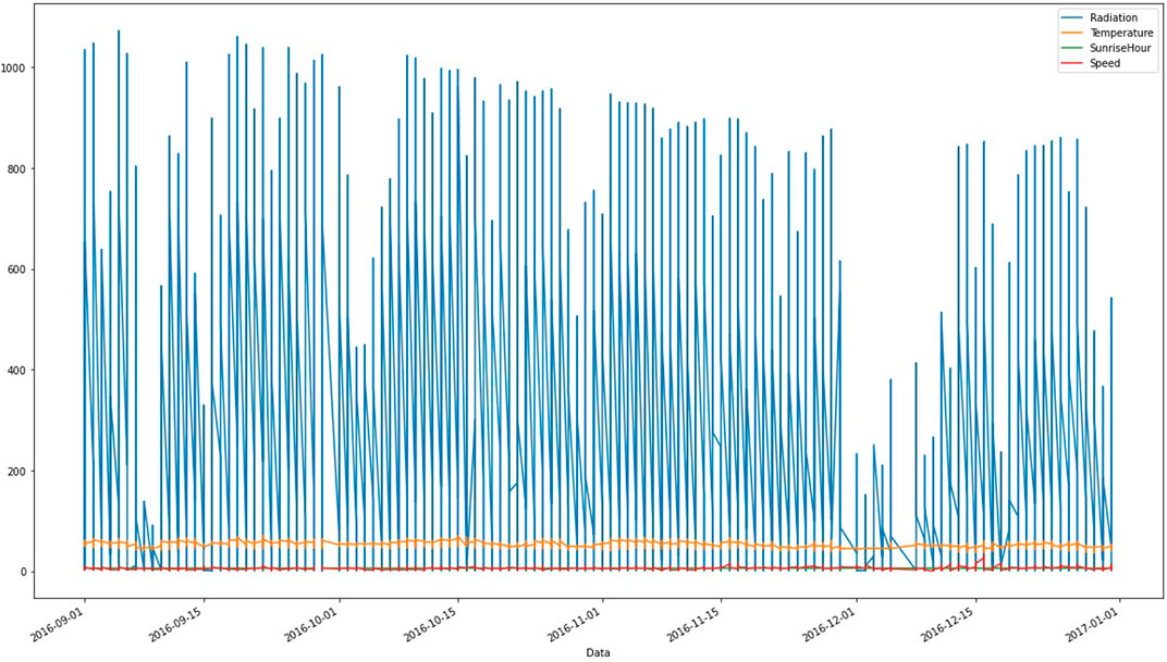
FIGURE 1. Distribution of parameter values of the tested dataset.

4 Experimental results

This section’s sole mission is to deliver an in-depth analysis of the investigation’s results, and that is exactly what it does. The investigations were conducted in a couple of different settings. The capabilities of the proposed binary ADSSOA for feature selection are addressed in the first scenario, and the capabilities of the algorithm for regression are illustrated in the second scenario. Both scenarios are applied to the dataset that is being evaluated. Both of these possible outcomes are detailed in the following section. Analyses and comparisons are performed on the ADSSOA method with respect to other algorithms that are regarded as being at the forefront of their fields, such as the squirrel search optimization algorithm (SS) (El-Kenawy et al., 2021), PSO (Bello et al., 2007), GWO (Khafaga et al., 2022), GA (El-Kenawy et al., 2020), firefly algorithm (FA) (Fister et al., 2012), and whale optimization algorithm (WOA) (Eid et al., 2021). As shown in Table 1, there is a presentation of the setup for the comparison algorithms, and in Table 2, there is a presentation of the ADSSOA configuration, which covers all of the experiment’s applicable parameters.

TABLE 1

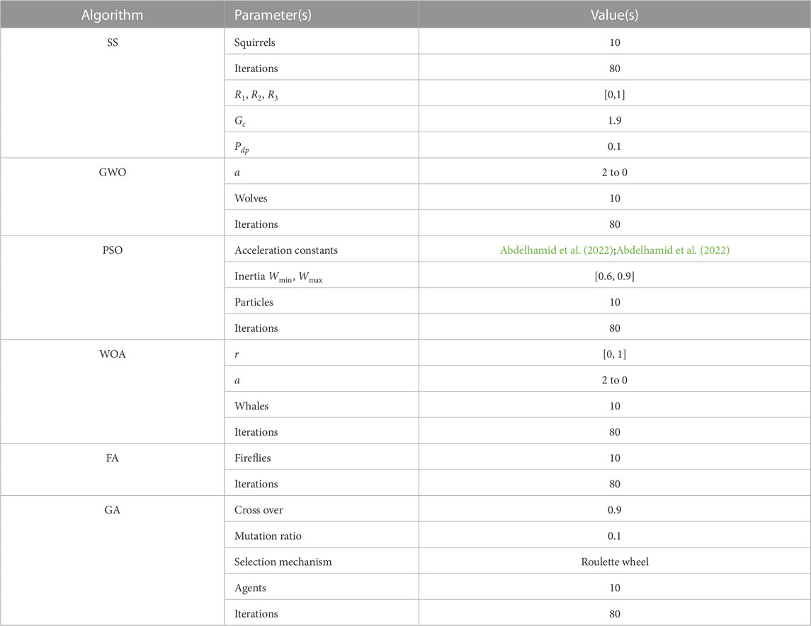
TABLE 1. Parameters used to set up compared algorithms.

TABLE 2

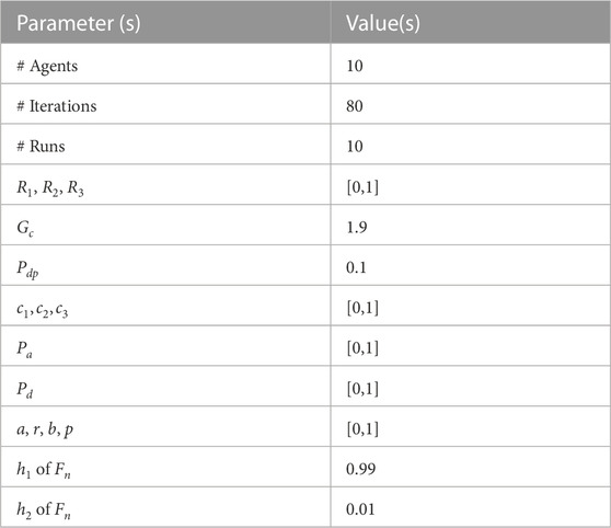
TABLE 2. Parameters used to set up the ADSSOA.

4.1 Feature selection scenario

When selecting features from the dataset, the proposed binary implementation of the ADSSOA method is used. The paper includes a discussion of the results of feature selection using the ADSSOA. The binary ADSSOA (bADSSOA) method is compared and contrasted with other binary optimization methods such as binary SS (bSS), binary WOA (bWOA), binary PSO (bPSO), binary GWO (bGWO), binary FA (bFA), and binary GA (bGA). Using the objective function presented in Eq 11, also known as F_n, the binary ADSSOA method can evaluate the quality of a given solution.

If a subset of features can be provided that results in a low classification error rate, then the approach is considered acceptable. The K-nearest neighbor (kNN) technique is a simple classification method that is commonly used. This method uses the K-nearest neighbor classifier, which ensures that the selected attributes are of high quality. The only criterion used in determining the classifiers is the shortest distance between the query instance and the training instances. This experiment does not utilize any models for the K-nearest neighbors in any way.

The proposed feature selection strategy’s effectiveness is measured according to the standards listed in Table 3. This table also includes a column labeled “M″ that indicates the total number of iterations performed by the proposed optimizer and its competitors. The symbol $S_j^{*}$ is used to represent the best solution, and the size of the best solution vector is represented by the value $size(S_j^{*})$. The total number of points for the test set is represented by the letter N. The predicted values are represented by the term $\widehat{V_n}$, while the actual values are represented by the term V_n.

TABLE 3

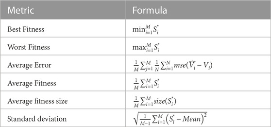
TABLE 3. Feature selection evaluation criteria to measure the effectiveness of feature selection methods.

The results of the feature selection process using the proposed and compared algorithms are displayed in Table 4. As shown in Table 2, these results are based on 80 iterations over 10 runs for 10 agents. The bADSSOA technique had an average error of (0.1801) and a standard deviation of (0.0656), performing as expected. The next best performing algorithms were bGWO with a score of (0.1973), bGA with a score of (0.2109), bFA with a score of (0.2295), bGA with a score of (0.5694), bWOA with a score of (0.2309), bPSO with a score of (0.2311), and bSS with a score of (0.2366) which had the lowest minimal average error in the feature selection process for the evaluated data. The bSS algorithm was the weakest one among all the available algorithms for feature selection.

TABLE 4

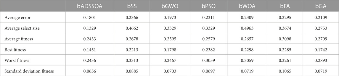
TABLE 4. Comparison of the proposed binary ADSSOA with other binary optimization algorithms.

Figure 2 illustrates the box plots of the average error for the bADSSOA and other optimization algorithms including bSS, bGWO, bPSO, bWOA, bFA, and bGA. The performance of the bADSSOA is measured using the objective function mentioned in Eq 11. The performance of the bADSSOA method compared to other optimization algorithms using a box plot that shows the histogram of average error for each algorithm is shown in Figure 3. Figure 4 displays the QQ plots, residual plots, and heat map for the bADSSOA and the other methods that were compared for the analyzed data, highlighting the correlation between the data and the quantiles and quantile differences.

FIGURE 2

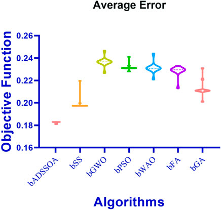
FIGURE 2. Comparing the performance of the bADSSOA method with other optimization algorithms. The average error for each algorithm is presented using a box plot.

FIGURE 3

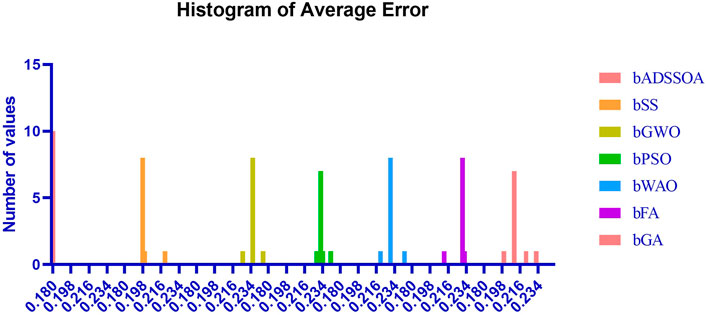
FIGURE 3. Comparing the performance of the bADSSOA method with other optimization algorithms using the histogram of average error.

FIGURE 4

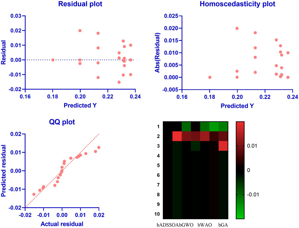
FIGURE 4. QQ and residual plots, along with a heat map, to analyze the performance of the bADSSOA and compare it with the other algorithms.

The statistical analysis uses one-way ANOVA and Wilcoxon signed-rank tests to determine the average error of the proposed binary ADSSOA. The Wilcoxon test is used to compare the proposed approach with other methods and determine if it outperforms them with a p-value of less than 0.05. The ANOVA test is also performed to determine if the proposed algorithm differs significantly from the others. The results of these tests are presented in Table 5 and Table 6, respectively. The analysis uses 10 rounds of each method to ensure reliable comparisons.

TABLE 5

TABLE 5. Outcomes of the ANOVA test that compared the proposed bADSSOA technique to the other examined algorithms.

TABLE 6

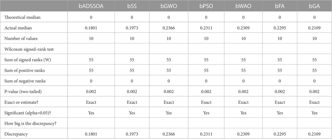
TABLE 6. Outcomes of the Wilcoxon signed-rank test that compared the proposed bADSSOA technique to the other examined algorithms.

4.2 Regression scenario

The optimal ensemble ADSSOA–LSTM model is compared to simpler models such as MLP, SVR, RF, k-NN, and LSTM over multiple runs and iterations with 10 agents. Additional metrics like RMSE, RRMSE, NSE, MAE, MBE, r, R2, and WI are used to evaluate the performance of the regression models. The dataset is represented by the N parameter, and the estimated and observed bandwidths are represented by $(\widehat{V_n})$ and (V_n), respectively. The arithmetic means of the estimated and observed values are represented by $(\overline{\widehat{V_n}})$ and (V_n), respectively. The evaluation criteria for predictions are outlined in Table 7.

TABLE 7

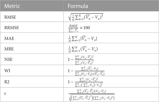
TABLE 7. Prediction evaluation criteria used in the regression scenario.

To further elaborate on the results, it is important to note that the ADSSOA–LSTM model outperformed not only the basic LSTM model but also other popular machine-learning models such as SVR, MLP, and RF based on the results presented in Table 8. The LSTM and MLP models had RMSE values of 0.001221 and 0.047336, respectively, while the ADSSOA–LSTM model had an RMSE of 0.000388, which was significantly higher than that of the other models. These results demonstrate the effectiveness of the proposed ADSSOA–LSTM model in optimizing the design of renewable energy systems and improving their performance. The study’s findings suggest that the hybrid approach combining the ADSSOA with LSTM can provide accurate predictions for renewable energy sources, which can help reduce the cost of energy production and improve energy efficiency.

TABLE 8

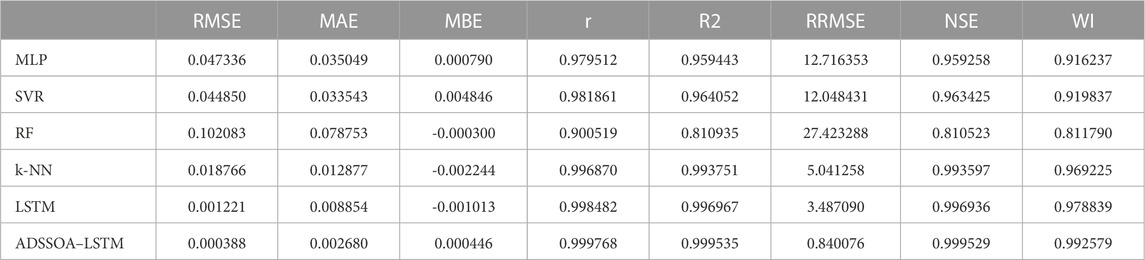
TABLE 8. Results of the suggested optimizing ADSSOA–LSTM model in comparison to basic models.

In the study, the proposed ADSSOA-based LSTM model is compared with several other popular swarm intelligence-based LSTM models such as SS, GWO, PSO, WOA, FA, and GA. The comparison is based on the RMSE of 10 individual runs for each algorithm. The RMSE results are presented in Table 9 along with a description of the proposed ADSSOA-based LSTM model. The table includes the minimum, median, maximum, and mean average errors for each algorithm. These results demonstrate the effectiveness of the proposed ADSSOA-based LSTM model compared to the other models in terms of accuracy in predicting hourly tilted solar irradiation.

TABLE 9

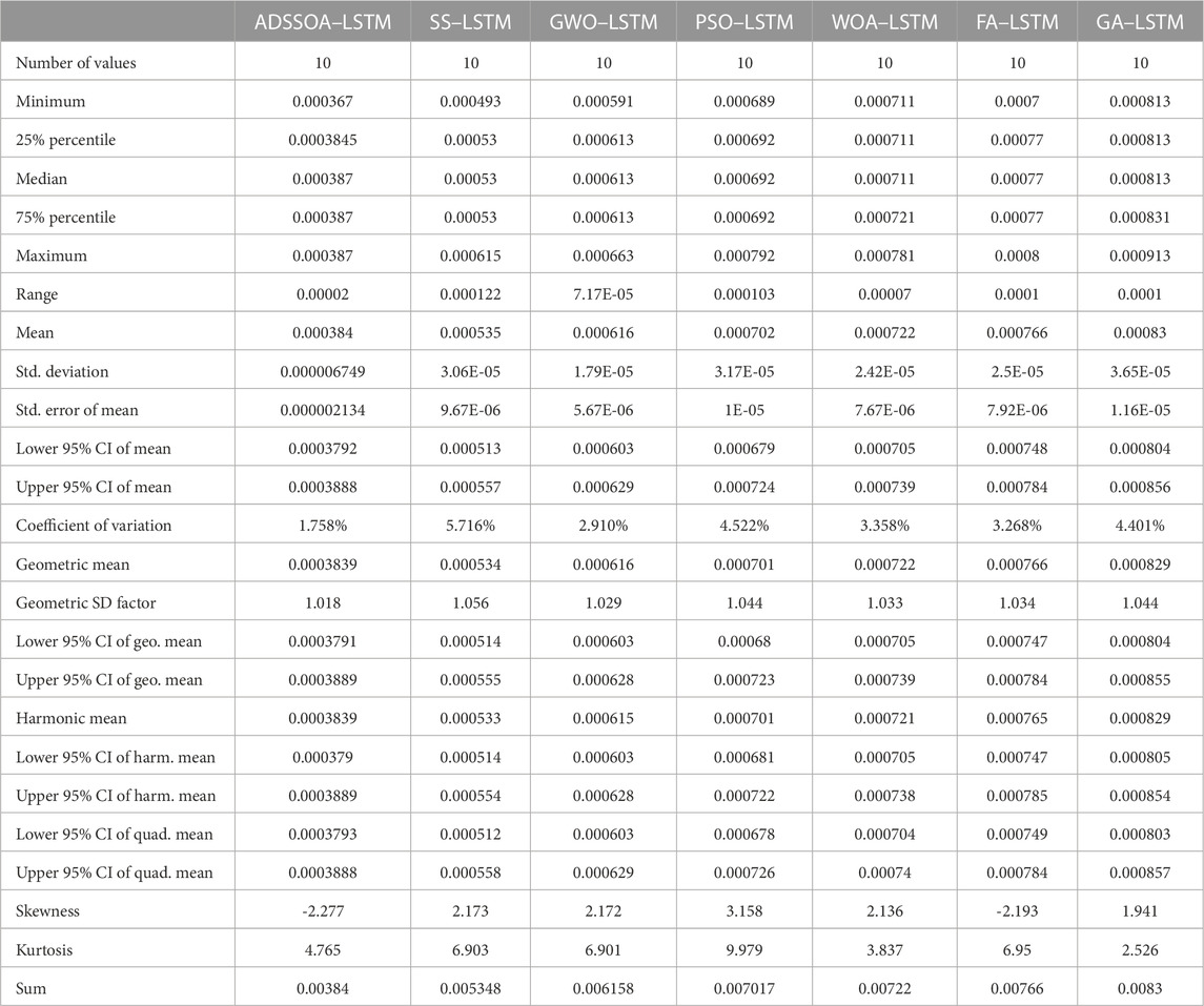
TABLE 9. Description of the proposed ADSSOA-based LSTM model and the results of other models from RMSE.

Figure 5 displays the box plot calculated using the RMSE for the proposed ADSSOA-based LSTM model as well as the SS, GWO, PSO, WOA, FA, and GA-based models. The quality of the optimized ensemble ADSSOA-based model, as shown in the figure, was determined with the help of the objective function described in Eq 11. Figure 6 shows the ROC curve of the presented ADSSOA versus the DTO algorithm. Figure 7 presents the QQ plots, residual plots, and heat map for both the ADSSOA-based model that was provided and the models that were compared for the investigated data. Both sets of plots are based on the analyzed data. These figures demonstrate that the given optimized ensemble ADSSOA-based model has the potential to outperform the models that were compared. The study’s statistical analysis was conducted using 10 individual iterations of each of the algorithms being presented and evaluated, ensuring that the comparisons are precise and the study results are trustworthy.

FIGURE 5

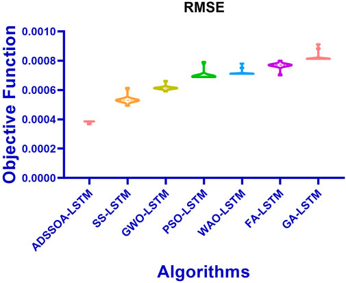
FIGURE 5. Box plot comparing the proposed ADSSOA-based LSTM model with other LSTM-based models. The comparison is based on RMSE.

FIGURE 6

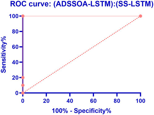
FIGURE 6. ROC curve of the proposed ADSSOA-based LSTM model compared to the SS-based LSTM model.

FIGURE 7

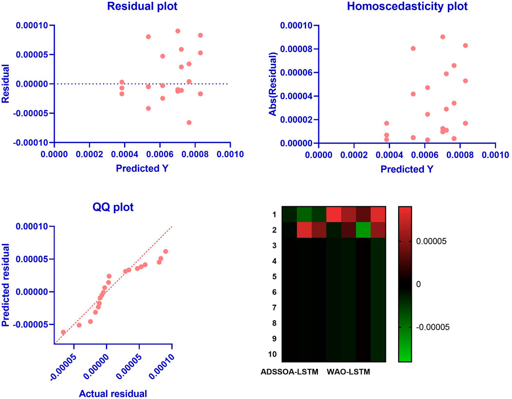
FIGURE 7. QQ plots, residual plots, and heat maps of the compared models and the proposed ADSSOA-based LSTM model.

The ANOVA test and the Wilcoxon signed-rank test are commonly used statistical methods to compare the performance of different models. In this study, both tests were used to evaluate the effectiveness of the proposed optimized ADSSOA–LSTM model compared to other models. Table 10 reports the results of the ANOVA test, which show that the proposed ADSSOA–LSTM model performs significantly better than the compared models. Table 11 further supports this claim by presenting the results of the Wilcoxon signed-rank test, which confirms that the proposed model outperforms the other models with statistical significance. The use of these statistical tests adds credibility to the findings of this study and highlights the superiority of the proposed model in accurately estimating hourly tilted solar irradiation.

TABLE 10

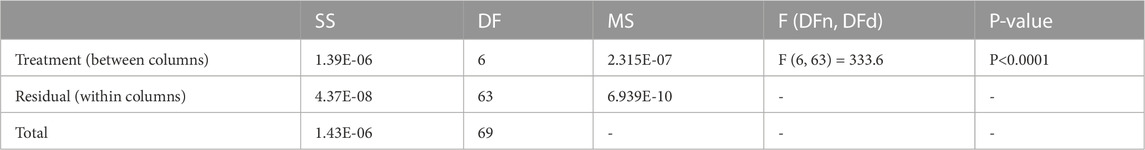
TABLE 10. Outcomes of the ANOVA test that compared the proposed ADSSOA–LSTM to other algorithms.

TABLE 11

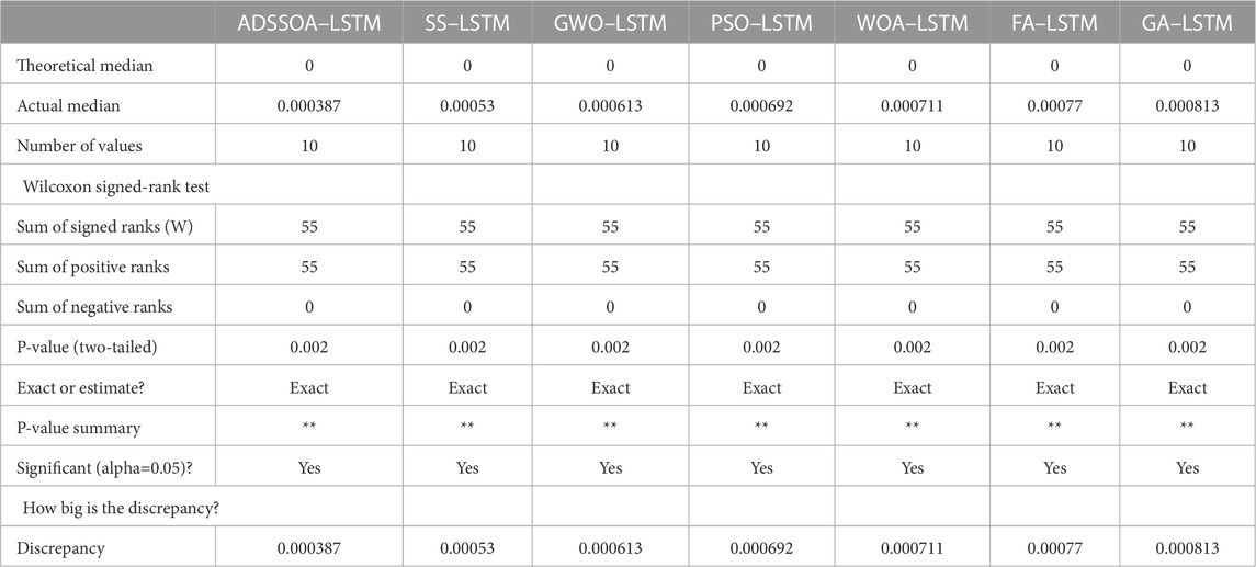
TABLE 11. Outcomes of the Wilcoxon signed-rank test that compared the proposed ADSSOA–LSTM to other algorithms.

5 Conclusion and future work

AI and ML techniques can improve performance and reduce the optimization time of renewable energy systems. The proposed hybrid ensemble-learning approach, which combines the ADSSOA with LSTM, is an innovative and promising solution. The use of ADSSOA, a novel swarm intelligence algorithm, enhances the optimization performance of the model. In contrast, using LSTM improves the predictions’ accuracy by capturing the data’s long-term dependencies. The results of the proposed approach demonstrate its superiority compared to other popular swarm intelligence algorithms, such as GA, PSO, and GWO, in terms of RMSE. The proposed model can be applied, in future, to other datasets and tasks related to renewable energy systems, such as wind speed prediction, power output estimation, and energy demand forecasting. Overall, the study contributes to advancing the field of renewable energy optimization and demonstrates the potential of AI and ML techniques in this domain. The proposed methodology achieved an average error of 0.1801, a standard deviation of 0.0656, and an RMSE of 0.000388 when compared to the other competing methods.

Data availability statement

The original contributions presented in the study are included in the article/Supplementary Material; further inquiries can be directed to the corresponding authors.

Author contributions

Conceptualization: E-SE-k ; methodology: E-SE-k and ME; software: DK; validation: AA; formal analysis: AA; investigation: ME; resources and writing—original draft preparation: AA and ME; writing—review and editing: E-SE-k; visualization: DK; supervision: E-SE-k; project administration: E-SE-k; and funding acquisition: AA. All authors contributed to the article and approved the submitted version.

Funding

This research project was funded by the Deanship of Scientific Research, Princess Nourah Bint Abdulrahman University, through the Program of Research Project Funding After Publication, grant no. 43-PRFA-P-62.

Conflict of interest

The authors declare that the research was conducted in the absence of any commercial or financial relationships that could be construed as a potential conflict of interest.

Publisher’s note

All claims expressed in this article are solely those of the authors and do not necessarily represent those of their affiliated organizations, or those of the publisher, the editors, and the reviewers. Any product that may be evaluated in this article, or claim that may be made by its manufacturer, is not guaranteed or endorsed by the publisher.

References

Abdelhamid, A. A., El-Kenawy, E.-S. M., Khodadadi, N., Mirjalili, S., Khafaga, D. S., Alharbi, A. H., et al. (2022). Classification of monkeypox images based on transfer learning and the al-biruni Earth radius optimization algorithm. Mathematics10, 3614. doi:10.3390/math10193614

CrossRef Full Text | Google Scholar

Ahmed, R., Sreeram, V., Mishra, Y., and Arif, M. (2020). A review and evaluation of the state-of-the-art in PV solar power forecasting: Techniques and optimization. Renew. Sustain. Energy Rev.124, 109792. doi:10.1016/j.rser.2020.109792

CrossRef Full Text | Google Scholar

Al-Hajj, R., Assi, A., and Fouad, M. M. (2018). “Forecasting solar radiation strength using machine learning ensemble,” in 2018 7th international conference on renewable energy research and applications (ICRERA) (IEEE). doi:10.1109/icrera.2018.8567020

CrossRef Full Text | Google Scholar

Almorox, J., Arnaldo, J., Bailek, N., and Martí, P. (2020). Adjustment of the angstrom-prescott equation from campbell-Stokes and kipp-zonen sunshine measures at different timescales in Spain. Renew. Energy154, 337–350. doi:10.1016/j.renene.2020.03.023

CrossRef Full Text | Google Scholar

Alrashidi, M., Alrashidi, M., and Rahman, S. (2021). Global solar radiation prediction: Application of novel hybrid data-driven model. Appl. Soft Comput.112, 107768. doi:10.1016/j.asoc.2021.107768

CrossRef Full Text | Google Scholar

Bellido-Jiménez, J. A., Gualda, J. E., and García-Marín, A. P. (2021). Assessing new intra-daily temperature-based machine learning models to outperform solar radiation predictions in different conditions. Appl. Energy298, 117211. doi:10.1016/j.apenergy.2021.117211

CrossRef Full Text | Google Scholar

Bello, R., Gomez, Y., Nowe, A., and Garcia, M. M. (2007). “Two-step particle swarm optimization to solve the feature selection problem,” in Seventh international conference on intelligent systems design and applications (ISDA), 691–696. doi:10.1109/ISDA.2007.101

CrossRef Full Text | Google Scholar

Belmahdi, B., Louzazni, M., and Bouardi, A. E. (2020). One month-ahead forecasting of mean daily global solar radiation using time series models. Optik219, 165207. doi:10.1016/j.ijleo.2020.165207

CrossRef Full Text | Google Scholar

Bouchouicha, K., Hassan, M. A., Bailek, N., and Aoun, N. (2019). Estimating the global solar irradiation and optimizing the error estimates under Algerian desert climate. Renew. Energy139, 844–858. doi:10.1016/j.renene.2019.02.071

CrossRef Full Text | Google Scholar

Browell, J., and Gilbert, C. (2020). “ProbCast: Open-source production, evaluation and visualisation of probabilistic forecasts,” in 2020 international conference on probabilistic methods applied to power systems (PMAPS) (IEEE). doi:10.1109/pmaps47429.2020.9183441

CrossRef Full Text | Google Scholar

Cao, Q., Liu, Y., Lyu, K., Yu, Y., Li, D. H., and Yang, L. (2020). Solar radiation zoning and daily global radiation models for regions with only surface meteorological measurements in China. Energy Convers. Manag.225, 113447. doi:10.1016/j.enconman.2020.113447

CrossRef Full Text | Google Scholar

[Dataset] (2017). Solar Radiation Prediction, task from nasa hackathon 2023. Avilable at: https://www.kaggle.com/dronio/SolarEnergy(Accessed 01 25.

Google Scholar

Demircan, C., Bayrakçı, H. C., and Keçebaş, A. (2020). Machine learning-based improvement of empiric models for an accurate estimating process of global solar radiation. Sustain. Energy Technol. Assessments37, 100574. doi:10.1016/j.seta.2019.100574

CrossRef Full Text | Google Scholar

Eid, M. M., El-kenawy, E.-S. M., and Ibrahim, A. (2021). “A binary sine cosine-modified whale optimization algorithm for feature selection,” in 2021 national computing colleges conference (NCCC) (IEEE). doi:10.1109/nccc49330.2021.9428794

CrossRef Full Text | Google Scholar

Eid, M. M., El-Kenawy, E.-S. M., Khodadadi, N., Mirjalili, S., Khodadadi, E., Abotaleb, M., et al. (2022). Meta-heuristic optimization of LSTM-based deep network for boosting the prediction of monkeypox cases. Mathematics10, 3845. doi:10.3390/math10203845

CrossRef Full Text | Google Scholar

El-kenawy, E.-S. M., Albalawi, F., Ward, S. A., Ghoneim, S. S. M., Eid, M. M., Abdelhamid, A. A., et al. (2022a). Feature selection and classification of transformer faults based on novel meta-heuristic algorithm. Mathematics10, 3144. doi:10.3390/math10173144

CrossRef Full Text | Google Scholar

El-Kenawy, E.-S. M., Eid, M. M., Saber, M., and Ibrahim, A. (2020). MbGWO-SFS: Modified binary grey wolf optimizer based on stochastic fractal search for feature selection. IEEE Access8, 107635–107649. doi:10.1109/access.2020.3001151

CrossRef Full Text | Google Scholar

El-Kenawy, E.-S. M., Mirjalili, S., Abdelhamid, A. A., Ibrahim, A., Khodadadi, N., and Eid, M. M. (2022b). Meta-heuristic optimization and keystroke dynamics for authentication of smartphone users. Mathematics10, 2912. doi:10.3390/math10162912

CrossRef Full Text | Google Scholar

El-Kenawy, E.-S. M., Mirjalili, S., Ibrahim, A., Alrahmawy, M., El-Said, M., Zaki, R. M., et al. (2021). Advanced meta-heuristics, convolutional neural networks, and feature selectors for efficient COVID-19 x-ray chest image classification. IEEE Access9, 36019–36037. doi:10.1109/access.2021.3061058

PubMed Abstract | CrossRef Full Text | Google Scholar

El-kenawy, E.-S. M., Mirjalili, S., Khodadadi, N., Abdelhamid, A. A., Eid, M. M., El-Said, M., et al. (2023). Feature selection in wind speed forecasting systems based on meta-heuristic optimization. PLOS ONE18, e0278491. doi:10.1371/journal.pone.0278491

PubMed Abstract | CrossRef Full Text | Google Scholar

Feng, Y., Hao, W., Li, H., Cui, N., Gong, D., and Gao, L. (2020). Machine learning models to quantify and map daily global solar radiation and photovoltaic power. Renew. Sustain. Energy Rev.118, 109393. doi:10.1016/j.rser.2019.109393

CrossRef Full Text | Google Scholar

Fister, I., Yang, X.-S., Fister, I., and Brest, J. (2012). Memetic firefly algorithm for combinatorial optimization. Tech. Rep.arXiv:1204.5165. Comments: 14 pages; Bioinspired Optimization Methods and their Applications (BIOMA 2012).

Google Scholar

Gupta, S., Katta, A. R., Baldaniya, Y., and Kumar, R. (2020). “Hybrid random forest and particle swarm optimization algorithm for solar radiation prediction,” in 2020 IEEE 5th international conference on computing communication and automation (ICCCA) (IEEE). doi:10.1109/iccca49541.2020.9250715

CrossRef Full Text | Google Scholar

Hossain, M., Mekhilef, S., Danesh, M., Olatomiwa, L., and Shamshirband, S. (2017). Application of extreme learning machine for short term output power forecasting of three grid-connected PV systems. J. Clean. Prod.167, 395–405. doi:10.1016/j.jclepro.2017.08.081

CrossRef Full Text | Google Scholar

Huynh, A. N.-L., Deo, R. C., An-Vo, D.-A., Ali, M., Raj, N., and Abdulla, S. (2020). Near real-time global solar radiation forecasting at multiple time-step horizons using the long short-term memory network. Energies13, 3517. doi:10.3390/en13143517

CrossRef Full Text | Google Scholar

Ibrahim, A., El-kenawy, E.-S. M., Kabeel, A. E., Karim, F. K., Eid, M. M., Abdelhamid, A. A., et al. (2023). Al-biruni Earth radius optimization based algorithm for improving prediction of hybrid solar desalination system. Energies16, 1185. doi:10.3390/en16031185

CrossRef Full Text | Google Scholar

Ibrahim, A., Noshy, M., Ali, H. A., and Badawy, M. (2020). Papso: A power-aware vm placement technique based on particle swarm optimization. IEEE Access8, 81747–81764. doi:10.1109/access.2020.2990828

CrossRef Full Text | Google Scholar

Khafaga, D. S., Alhussan, A. A., El-Kenawy, E.-S. M., Ibrahim, A., Eid, M. M., and Abdelhamid, A. A. (2022). Solving optimization problems of metamaterial and double t-shape antennas using advanced meta-heuristics algorithms. IEEE Access10, 74449–74471. doi:10.1109/access.2022.3190508

CrossRef Full Text | Google Scholar

Khosravi, A., Koury, R., Machado, L., and Pabon, J. (2018a). Prediction of hourly solar radiation in abu musa island using machine learning algorithms. J. Clean. Prod.176, 63–75. doi:10.1016/j.jclepro.2017.12.065

CrossRef Full Text | Google Scholar

Khosravi, A., Nunes, R., Assad, M., and Machado, L. (2018b). Comparison of artificial intelligence methods in estimation of daily global solar radiation. J. Clean. Prod.194, 342–358. doi:10.1016/j.jclepro.2018.05.147

CrossRef Full Text | Google Scholar

Li, J., Guo, Y., Platt, G., and Ward, J. K. (2013). Renewable energy aggregation with intelligent battery controller. Renew. Energy59, 220–228. doi:10.1016/j.renene.2013.03.027

CrossRef Full Text | Google Scholar

Li, J., Ward, J. K., Tong, J., Collins, L., and Platt, G. (2016). Machine learning for solar irradiance forecasting of photovoltaic system. Renew. Energy90, 542–553. doi:10.1016/j.renene.2015.12.069

CrossRef Full Text | Google Scholar

Marzouq, M., Fadili, H. E., Lakhliai, Z., and Zenkouar, K. (2017). A review of solar radiation prediction using artificial neural networks. In 2017 international conference on wireless technologies, embedded and intelligent systems (WITS) (IEEE). doi:10.1109/wits.2017.7934658

CrossRef Full Text | Google Scholar

Mishra, S., and Palanisamy, P. (2018). Multi-time-horizon solar forecasting using recurrent neural network. In 2018 IEEE energy conversion congress and exposition (ECCE) (IEEE). doi:10.1109/ecce.2018.8558187

CrossRef Full Text | Google Scholar

Narvaez, G., Giraldo, L. F., Bressan, M., and Pantoja, A. (2021). Machine learning for site-adaptation and solar radiation forecasting. Renew. Energy167, 333–342. doi:10.1016/j.renene.2020.11.089

CrossRef Full Text | Google Scholar

Pang, Z., Niu, F., and O’Neill, Z. (2020). Solar radiation prediction using recurrent neural network and artificial neural network: A case study with comparisons. Renew. Energy156, 279–289. doi:10.1016/j.renene.2020.04.042

CrossRef Full Text | Google Scholar

Praynlin, E., and Jensona, J. I. (2017). Solar radiation forecasting using artificial neural network. In 2017 innovations in power and advanced computing technologies (i-PACT) (IEEE). doi:10.1109/ipact.2017.8244939

CrossRef Full Text | Google Scholar

Quaiyum, S., Rahman, S., and Rahman, S. (2011). Application of artificial neural network in forecasting solar irradiance and sizing of photovoltaic cell for standalone systems in Bangladesh. Int. J. Comput. Appl.32, 51–56. Full text available.

Google Scholar

Sobri, S., Koohi-Kamali, S., and Rahim, N. A. (2018). Solar photovoltaic generation forecasting methods: A review. Energy Convers. Manag.156, 459–497. doi:10.1016/j.enconman.2017.11.019

CrossRef Full Text | Google Scholar

Voyant, C., Notton, G., Kalogirou, S., Nivet, M.-L., Paoli, C., Motte, F., et al. (2017). Machine learning methods for solar radiation forecasting: A review. Renew. Energy105, 569–582. doi:10.1016/j.renene.2016.12.095

CrossRef Full Text | Google Scholar

Wang, H., Liu, Y., Zhou, B., Li, C., Cao, G., Voropai, N., et al. (2020). Taxonomy research of artificial intelligence for deterministic solar power forecasting. Energy Convers. Manag.214, 112909. doi:10.1016/j.enconman.2020.112909

CrossRef Full Text | Google Scholar

Yadav, A. K., and Chandel, S. (2014). Solar radiation prediction using artificial neural network techniques: A review. Renew. Sustain. Energy Rev.33, 772–781. doi:10.1016/j.rser.2013.08.055

CrossRef Full Text | Google Scholar

Zhou, Y., Liu, Y., Wang, D., Liu, X., and Wang, Y. (2021). A review on global solar radiation prediction with machine learning models in a comprehensive perspective. Energy Convers. Manag.235, 113960. doi:10.1016/j.enconman.2021.113960

CrossRef Full Text | Google Scholar

Glossary