Fast prediction of compressor flow field in nuclear power system based on proper orthogonal decomposition and deep learning

Research and development on digital twins of nuclear power systems has focused on high-precision real-time simulation and the prediction of local complex three-dimensional fluid dynamics. Traditional computational fluid dynamics (CFD) methods cannot take into consideration the efficiency and accuracy of fluid dynamics. In this study, a fast-flow field-prediction framework based on proper orthogonal decomposition (POD) and deep learning is proposed. Compressed data containing the original flow field information are obtained using POD and deep neural network (DNN) is used to construct the POD-DNN flow field reduction model to achieve fast flow field prediction. The calculation accuracy and speed of the reduced-order model are analyzed in detail, considering the flow field of the nuclear compressor and key flow equipment of the nuclear power system as objects. The results show that the average relative deviation of the POD-DNN is <10% and calculation time is <1% when compared to those of CFD. This research shows that the high-fidelity model constructed using model reduction and deep learning is a feasible method for the realization of digital twins of the nuclear power system in engineering.

1 Introduction

With the development of digital technology, a comprehensive and full-cycle digital simulation of nuclear power systems could reduce the cost of research and development of reactors and improve safety and economy of future reactors. Building a digital twin of a nuclear power system through multi-professional and multi-scale real-time/ultra real-time simulation, virtual–real interactive feedback, data fusion analysis, decision iterative optimization, intelligent control, and other methods that could reflect the entire life cycle of physical equipment and provide support for research and development, operation, and maintenance are all the ultimate goal.

Whether the digital twin of a nuclear power system can accurately reflect and predict the operational state of the physical nuclear power system in real time depends on an efficient and accurate description of the complex thermal and hydraulic problems present in it. The accurate and real-time simulation of local three-dimensional flow fields is difficult. The traditional method adopts computational fluid dynamics (CFD) and a system program for multi-scale coupling simulations. However, obtaining a numerical solution through CFD is complex and computationally expensive. The real-time simulation requirements of the digital twin of a reactor system based on CFD cannot be met with the advancements in supercomputer technology achieved so far. Therefore, it is necessary to develop a flow field reduced-order model (ROM) that not only provides accuracy similar to that of the CFD solution but is also computationally efficient.

In recent years, the rapid development of machine learning (ML) technology has demonstrated a strong ability to predict non-linear problems. Deep learning (DL) is the latest development direction in ML and was first proposed by Marton and Säaljö (1976). The DL model is characterized by the use of multilayer neural networks to unify various algorithms in ML, and each layer of a neural network can map the input non-linearly. The earliest application of DL in solving flow problems was by Ling et al. (2016) of Sandia National Laboratories in the United States, who built a DL network for the Reynolds mean turbulence model by embedding Galileo invariants into a deep neural network (DNN) and predicted Reynolds stress, pipeline flow, and velocity field. Since 2016, ML and DL have been applied to typical flow problems such as flow field morphology, pressure field distribution, and temperature field diffusion (Miyanawala and Jaiman, 2017; Maulik et al., 2019; Sekar et al., 2019; Xinyu et al., 2019; Xie et al., 2020; Yuan et al., 2020; Li Y. et al., 2021; Li et al., 2021b; Chen et al., 2021; Morimoto et al., 2021). Most of these works are aimed at simple two-dimensional flow problems, and hence, the results of numerical calculations of the full flow field can be directly used as the training data set. However, data from the numerical calculations of the flow field in actual engineering are very large, and the training of neural networks often requires very high computing resources (Xinyu et al., 2019), leading to difficulty in providing reasonable prediction results.

ROMs for low-dimensional feature extraction and analysis have been established and widely used for the morphological recognition of flow fields and prediction of dynamic characteristics (Chunyu et al., 2019), considering the problem of their high data dimensions. Model downgrading is a key technique for transferring highly detailed and complex simulation models to other areas and life cycle phases, which is achieved by reducing the degrees of freedom, that is, by improving the speed of model execution while maintaining the required accuracy and predictability. Model reduction is one of the core technologies of digital twinning, which can compress the simulation model for real-time simulation and reuse it in the early stages of product development and later stages of the product life cycle, particularly in the product operation and maintenance stages.

A variety of mathematical projection methods in linear algebra, such as proper orthogonal decomposition (POD) (Sirovich, 1987; Chen et al., 2015; Chunyu et al., 2019; San, O. et al., 2018) and dynamic mode decomposition (Schmid, 2010), have been proposed and used for the linearization analysis of flow fields. For example, Taira et al. (2020) selected cylinder wakes, wall-bounded flows, airfoil wakes, and cavity flows, and proved that the reduced-order mode can be used for the characteristic analysis of flow problems. Many researchers have combined model reduction with DL to explore a new method of flow field prediction. Bukka et al. (2021) proposed an unsteady flow field prediction tool that combines model reduction and DL. Yousif and Lim (2022) used ROM and DL algorithms to predict the flow field around a wall-mounted square column. Gupta and Jaiman (2022) used a POD-DNN model to predict fluid dynamics and vortex shedding patterns in three-dimensional spheres. They used DL based on physical simulation data and compared it to a full-order prediction (i.e., CFD) that significantly improved the speed of online prediction and provided a new method of rapid prediction for digital twin reactor flow fields. However, most of the current research focuses on two-dimensional geometry and a simple flow field, and more application-oriented research is required.

This study proposes to combine the advantages of model reduction technology in describing high-dimensional problems and the ability of DL methods to predict non-linear problems. Taking the flow field of a compressor, which is the key flow equipment of the nuclear power system, as the object, the flow field prediction of the compressor based on POD-DNN is studied, the ROM model suitable for the flow field prediction of the nuclear compressor is developed, and the accuracy and efficiency of ROM prediction are evaluated. This lays the foundation for the research and development of real-time and ultra real-time digital twins of nuclear power systems in the future.

2 Reduced-order model based on POD and DNN

2.1 POD-based fluid dynamics reduction

The POD-based flow field reduction method achieves model reduction by appropriately truncating the contribution of the eigenvalue in the POD feature space. For a particular flow field data set {$u^k$}, $u^k$ can be obtained experimentally or numerically. The goal of the POD method is to find a canonical set of orthogonal bases {${\varphi }_i$} in the data set $u^k$ and maximize the projection of the elements of the data set $u^k$ on this basis.

In the fluid dynamics problem, the abovementioned process is realized as follows. The velocity field $u\left(x,t\right)$ is decomposed into the superposition of the average velocity $u_0$ and pulsating velocity $u^{\prime }\left(x,t\right)$:

$\mathit{u}\left(\mathit{x},\mathit{t}\right)={\mathit{u}}_0+{\mathit{u}}^{\prime }\left(\mathit{x},\mathit{t}\right).(1)$

The pulsating velocity $u^{\prime }\left(x,t\right)$ was decoupled over the temporal and spatial domains and projected onto a set of spatially orthogonal basis {${\varphi }_i$}.

${\mathit{u}}^{\prime }\left(\mathit{x},\mathit{t}\right)={\displaystyle \sum _{\mathit{n}=1}^{\infty }}{\mathit{a}}_{\mathit{n}}\left(\mathit{t}\right){\mathit{\phi }}_{\mathit{n}}\left(\mathit{x}\right).(2)$

Substituting Eq. 2 into Eq. 1, we get

$\mathit{u}\left(\mathit{x},\mathit{t}\right)={\mathit{u}}_0+{\displaystyle \sum _{\mathit{n}=1}^{\infty }}{\mathit{a}}_{\mathit{n}}\left(\mathit{t}\right){\mathit{\phi }}_{\mathit{n}}\left(\mathit{x}\right)={\displaystyle \sum _{\mathit{n}=0}^{\infty }}{\mathit{a}}_{\mathit{n}}\left(\mathit{t}\right){\mathrm{\phi }}_{\mathit{n}}\left(\mathit{x}\right),(3)$

where $a_0\left(t\right)=1$ and ${\phi }_0\left(x\right)=u_0$. The pulsation of the velocity can be regarded as the result of the linear superposition of a set of time-independent spatial functions ${\phi }_n\left(x\right)$ which changes over time according to the corresponding coefficient $a_n\left(t\right)$. For the convenience of a mathematical form, the space basis ${\phi }_n\left(x\right)$ is artificially defined to have orthogonal normality on the fluid domain Ω of the calculation as follows:

${\mathit{\phi }}_{\mathit{i}}\left(\mathit{x}\right)\bullet {\mathit{\phi }}_{\mathit{j}}\left(\mathit{x}\right)=\underset{\mathit{\Omega }}{\iiint }{\mathit{\phi }}_{\mathrm{i}}\left(\mathit{x}\right){\mathit{\phi }}_{\mathit{j}}\left(\mathit{x}\right)\mathit{d}\mathit{V}=\left\{\begin{array}{c}1\mathit{i}=\mathit{j}\\ 0\mathit{i}\ne \mathit{j}\end{array}\right..(4)$

A correlation matrix $\mathbf{C}=\left({\mathbf{C}}^{\mathrm{m}\mathrm{n}}\right)$ of the second-order statistical fluctuation is defined in the orthogonal decomposition reduction method and is used to describe the autocorrelation of any two points.

${\mathit{C}}^{\mathit{m}\mathit{n}}≔\frac{\mathbf{1}}{\mathit{M}}{\left({\mathit{u}}^{\mathit{m}}-{\mathit{u}}_{\mathbf{0}},{\mathit{u}}^{\mathit{n}}-{\mathit{u}}_{\mathbf{0}}\right)}_{\mathit{\Omega }}.(5)$

This statistic has no physical meaning in the flow field, but its magnitude characterizes the pulsating kinetic energy of the flow field to some extent (Yousif and Lim, 2022). Considering the calculation of the pulsating kinetic energy ${\mathrm{E}}_{\mathrm{T}}$ of the flow field with the number of steps m, its expression becomes

${\mathit{E}}_{\mathit{T}}=\frac{\mathbf{1}}{\mathbf{2}}\underset{\mathit{\Omega }}{{\displaystyle \int }}〈{\mathit{u}}^{\prime }{\left(\mathit{x},\mathit{t}\right)}^{\mathbf{2}}〉\mathit{d}\mathit{V}=\frac{\mathbf{1}}{\mathbf{2}\mathit{m}}{\displaystyle \sum _{\mathit{i}=\mathbf{1}}^{\mathit{m}}}\underset{\mathit{\Omega }}{{\displaystyle \int }}{\mathit{u}}^{\prime }{\left(\mathit{x},{\mathit{t}}_{\mathit{i}}\right)}^{\mathbf{2}}\mathit{d}\mathit{V}.(6)$

Substituting Eq. 2 in Eq. 6 and simplifying it according to Eq. 4 yields

$\begin{array}{c}{\mathit{E}}_{\mathit{T}}=\frac{1}{2}{\displaystyle \sum _{\mathit{n}=1}^{\mathit{\infty }}}{{\mathit{a}}_{\mathit{n}}}^2=\frac{1}{2}{{\displaystyle \sum _{\mathit{n}=1}^{\mathit{\infty }}}\left[\frac{1}{\mathit{m}}{\displaystyle \sum _{\mathit{i}=1}^{\mathit{m}}}{\mathit{a}}_{\mathit{n}}\left({\mathit{t}}_{\mathit{i}}\right)\right]}^2\\ ={\displaystyle \sum _{\mathit{n}=1}^{\mathit{\infty }}}\frac{1}{2{\mathit{m}}^2}{\left[{\displaystyle \sum _{i=1}^{\mathit{m}}}{\mathit{a}}_{\mathit{n}}\left({\mathit{t}}_{\mathit{i}}\right)\right]}^2={\displaystyle \sum _{\mathit{n}=1}^{\mathit{\infty }}}{\mathit{\lambda }}_{\mathit{n}},\end{array}(7)$

where ${\mathrm{\lambda }}_{\mathrm{n}}$ represents the pulsating kinetic energy contained in each characteristic space base (mode). ${\mathrm{\lambda }}_{\mathrm{n}}$ is arranged in the descending order to obtain a new sequence: ${\mathrm{\lambda }}_{\mathrm{n}}\left({\mathrm{\lambda }}_1>{\mathrm{\lambda }}_2>{\mathrm{\lambda }}_3>\cdots \right)$, and the bases corresponding to these terms ${\phi }_n$ are POD bases.

We set the number of discrete units of the flow field as m and the number of snapshot samples as n, and traverse all discrete units and time steps of the flow field using the abovementioned process.

$\frac{\mathbf{1}}{\mathit{n}}\mathit{U}{\mathit{U}}^{\mathit{T}}\mathit{W}\mathit{\phi }=\mathit{\lambda }\mathit{\phi },(8)$

where $U\in R^{m\times n}$, $U_{ij}=u^{\prime }\left(x_i,t_j\right)\left(i=1,\dots .,m,j=1,\dots \dots ,n\right)$, $W\in R^{m\times m}$, $W_{ij}=∆V_i{\delta }_{ij}$, and $∆V_i$ are the discrete cell volume. This formula is equivalent to

$\frac{1}{\mathit{n}}{\mathit{U}}^{\mathit{T}}\mathit{W}\mathit{U}{\mathit{\psi }}_{\mathit{n}}={\mathit{\lambda }}_{\mathit{n}}{\mathit{\psi }}_{\mathit{n}},(9)$

$\mathit{\phi }=\frac{1}{\sqrt{{\mathit{\lambda }}_{\mathit{n}}}}\mathit{U}{\mathit{\psi }}_{\mathit{n}}.(10)$

Equation 9 significantly reduces the computation of the eigenvalues and eigenvectors by matrix decomposition. It can be seen that the maximum number of bases that can be used for the flow field order-reduction model is the number of snapshot samples. To ensure the accuracy of the order reduction calculation under the condition of saving computing resources, the number of POD bases that can be used for flow field reduction was set as $N_{POD}$ and the number of POD bases that can be used for intercepting was set as $N_{used}\left(0<N_{used}\le N_{POD}\right)$ in order to define the magnitude of the cumulative pulsating kinetic energy that characterizes the selected POD base.

$\mathit{\eta }=\frac{{\displaystyle \mathit{\sum }_{\mathit{n}\mathit{=}\mathbf{1}}^{{\mathit{N}}_{\mathit{u}\mathit{s}\mathit{e}\mathit{d}}}}{\mathit{\lambda }}_{\mathit{n}}}{{\displaystyle \mathit{\sum }_{\mathit{n}\mathit{=}\mathbf{1}}^{{\mathit{N}}_{\mathit{P}\mathit{O}\mathit{D}}}}{\mathit{\lambda }}_{\mathit{n}}}.(11)$

When $N_{\mathrm{u}\mathrm{s}\mathrm{e}\mathrm{d}}$ is larger, η is closer to 1, and the reduction effect of the flow field is better; however, the calculation cost is higher and vice versa. Therefore, it is necessary to select a reasonable number of $N_{\mathrm{u}\mathrm{s}\mathrm{e}\mathrm{d}}$ based on the actual situation and requirements.

2.2 Deep neural network

In this study, a back-propagation neural network (BPNN) proposed by Rumelhart (1986) was used to predict the flow field based on POD (Xie et al., 2020). This is a multilayer feedforward network that minimizes the error mean square between the expected and actual outputs of the model through a gradient search. The BPNN has a mature theory, superior performance, and wide applicability.

A neural network is based on the extension of a perceptron. A perceptron (Figure 1) is a linear classification model with several inputs and one output. It is composed of two main parts: an adder that weighs all inputs to the neuron:

$\mathit{z}=\sum {\mathit{w}}_1{\mathit{x}}_{\mathit{i}}+\mathit{b},(12)$

and a processing unit that produces an output based on a predefined function called the activation function $\phi \left(z\right)$. Each neuron has its own set of weights and thresholds (bias), which it learns through different learning algorithms.

FIGURE 1

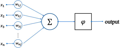
FIGURE 1. Perceptron.

Multiple perceptrons are connected such that all perceptron inputs are the same, but after adjustment, only one perceptron outputs at a time, forming a multivariate classifier. This structure is called an artificial neural network (ANN). The DNN can be understood as the neural network of many hidden layers. According to the location of different layers, the neural network layers inside the DNN can be classified into input, hidden, and output layers, and these are fully connected (Figure 2).

FIGURE 2

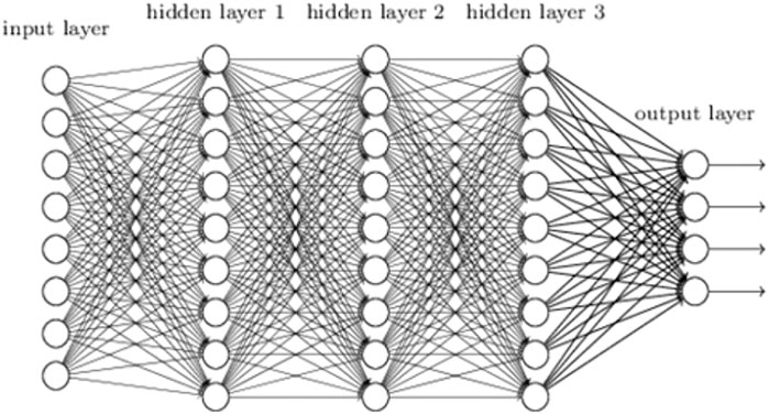
FIGURE 2. Deep neural network.

The recommended form of the activation function in modern neural networks is as follows:

$\mathit{\phi }\left(\mathit{z}\right)=\mathit{max}\left\{0,\mathit{z}\right\}.(13)$

This is called a rectified linear unit (ReLU) (Jarrett et al., 2009; Nair and Hinton, 2010; Glorot et al., 2011). The ReLU is the recommended activation function by default for most feedforward neural networks. As the function is close to linear, it is easier to use a gradient-based optimization algorithm that is used for linear models. The training process of the neural network was realized using a quadratic function that minimized the output error. The training process of the neural network can be described using the following mathematical procedure.

The loss function is defined as the real value of all sample points ${\widehat{y}}_i$ and the predicted deviation between $y_i$, which guides the direction of the training of the neural network. Mean squared error loss (MSE_loss) is the most commonly used loss function in ML and DL, and its form is as follows:

${\mathit{J}}_{\mathit{M}\mathit{S}\mathit{E}}=\frac{1}{\mathit{N}}{\displaystyle \sum _{\mathit{i}=1}^{\mathit{N}}}{\left({\mathit{y}}_{\mathit{i}}-{\widehat{\mathit{y}}}_{\mathit{i}}\right)}^2.(14)$

The loss function shows the current performance of the neural network model. The process of using the loss function to train the neural network and minimize the value of the loss function is called optimization. The process of the optimization algorithm, which is based on gradient descent, is as follows:

Calculate the θ gradient of the loss function with respect to

${\mathit{g}}_{\mathit{t}}={\mathit{\nabla }}_{\mathit{\theta }}\mathit{J}\left(\mathit{\theta }\right).(15)$

The first-order momentum m_t and second-order momentum ${\upsilon }_t$ are calculated based on the historical gradient values. The variable momentum is set as a negative gradient of the exponential decaying (Wilson et al., 2017) as follows:

${\mathit{m}}_{\mathit{t}}=\mathit{\varphi }\left({\mathit{g}}_1,{\mathit{g}}_2,...,{\mathit{g}}_{\mathit{t}}\right),(16)$

${\mathit{\upsilon }}_{\mathit{t}}=\mathit{\psi }\left({\mathit{g}}_1,{\mathit{g}}_2,...,{\mathit{g}}_{\mathit{t}}\right).(17)$

Updated network parameters are as follows:

${\mathit{\theta }}_{\mathit{t}+1}={\mathit{\theta }}_{\mathit{t}}-\frac{1}{\sqrt{{\mathit{\upsilon }}_{\mathit{t}}+\mathit{\epsilon }}}{\mathit{m}}_{\mathit{t}},(18)$

where the small quantity $\epsilon$ is used to avoid a denominator of 0.

In this study, adaptive momentum estimation (Adam) (Kingma and Ba, 2014) and stochastic gradient descent (SGD) algorithms (Bottou, 1998) are used. Adam is an extension of the SGD algorithm, which uses an independent adaptive learning rate to determine the hyperparameters that are more robust.

For the SGD algorithm, we used the following momentum:

${\mathit{m}}_{\mathit{t}}=\mathit{\gamma }{\mathit{m}}_{\mathit{t}-1}+\mathit{\eta }{\mathit{g}}_{\mathit{t}},(19)$

${\mathit{\upsilon }}_{\mathit{t}}={\mathit{I}}^2,(20)$

$\mathit{\epsilon }=0.(21)$

The superparameter $\gamma$ determines the contribution of the past gradient’s exponential decaying to the training rate, and $\eta$ is the learning rate.

For the Adam algorithm,

${\mathit{m}}_{\mathit{t}}=\mathit{\eta }\left[{\mathit{\beta }}_1{\mathit{m}}_{\mathit{t}-1}+\left(1-{\mathit{\beta }}_1\right){\mathit{g}}_{\mathit{t}}\right],(22)$

${\mathit{\upsilon }}_{\mathit{t}}={\mathit{\beta }}_2{\mathit{\upsilon }}_{\mathit{t}-1}+\left(1-{\mathit{\beta }}_2\right){\mathit{g}}_{\mathit{t}}^2,(23)$

where ${\beta }_1$ and ${\beta }_2$ are the exponential decaying rates of the estimation of the first- and second-order momenta, respectively.

2.3 Reduced-order model of flow fields based on POD and DNN

According to the POD method described in Section 2.1, dimensionality reduction was performed on the data matrix of the flow field variables, and the main modes and modal coefficients of the flow field were extracted. The mode coefficient after order-reduction was used for DNN training to directly predict the mode coefficient under unknown conditions and reconstruct the flow field on a POD orthogonal basis. This process avoids solving higher-order non-linear partial differential equations and helps achieve real-time prediction of the local flow field.

The POD-DNN method consists of three parts as shown in Figure 3: (A) acquisition of flow field snapshot data, (B) creation of POD-DNN, and (C) use of POD-DNN for forecasting. This process involves the following steps: (1) sample acquisition: flow field measurements, such as laser particle image velocimetry, or CFD codes, such as OpenFOAM and Fluent, are used to obtain simulation data during the creation of the ROM. (2) The variable matrix of the flow field is decomposed by POD, the order of the flow field is reduced, and the POD mode and mode coefficients are obtained. (3) Taking the boundary conditions as input and variable data after reduced order as output, the POD-DNN model of flow field prediction is finally obtained through the training of the neural network, and verification and optimization of the test sample set. (4) The neural network was used to predict the flow field and output the POD modal coefficient under the predicted conditions. (5) Based on POD, the flow field variables are reconstructed after order reduction to achieve flow field restoration, and the flow field variables in a matrix form are obtained.

FIGURE 3

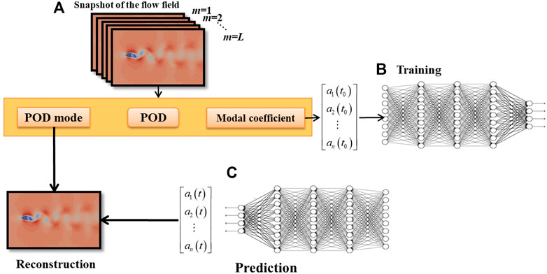
FIGURE 3. Creation of proper orthogonal decomposition–deep neural network (POD–DNN) and prediction process of neural networks. (A) Acquisition of flow field snapshot data, (B) creation of POD-DNN, and (C) use of POD-DNN for forecasting.

2.4 Preliminary verification of POD-DNN flow field prediction model

The cylindrical flow around the cylinder shown in Figure 4 was considered to analyze the prediction effect of the POD-DNN flow field prediction model. CFD was used to obtain flow field data for 100 different operating conditions (inlet Reynolds number). A total of 100 time steps were calculated for each operating condition point, and 50 of them were randomly selected as the sample data, namely, the training set. The first 20 orders of the main modes and time coefficients after the POD decomposition were used to reconstruct the training data of the flow field and ROM.

FIGURE 4

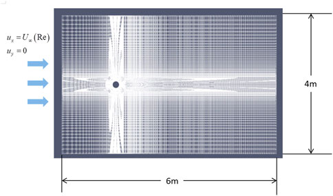
FIGURE 4. Mesh model of cylindrical flow.

The DNN forward propagation algorithm provided by the PyTorch platform was used for training. Six layers of the neural network were set, SGD was selected by the optimizer, the learning rate was set to 0.00002, the number of training was set to 3,000, and the training took 30 s. The reduction in the data scale significantly improved the training efficiency of the neural network.

The flow field results predicted by the POD-DNN are shown in Figure 5. A comparison between the ROM and instantaneous velocity field calculated using CFD at the 45th operating condition point is provided. By comparing the original flow field with the predicted flow field, it can be seen that the neural network successfully predicts the basic characteristics of the flow field. The ROM was in good agreement with the velocity field distribution calculated using the CFD. The ROM obtains the von Karman vortex street formed by the downstream flow field of the cylinder, and the local velocity in the wake region is slightly different from that of the CFD result.

FIGURE 5

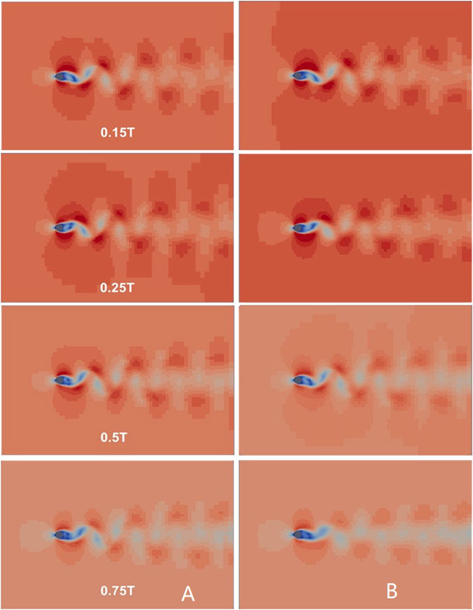
FIGURE 5. Comparison of velocity fields predicted by (A) computational fluid dynamics and (B) reduced-order model at 0.15, 0.25, 0.5, and 0.75 T, and Reynolds number Re = 98.

By calculating the average relative deviation between the predicted and real values of each mesh quantity, the accuracy of the POD-DNN is quantitatively analyzed after the reconstructed flow field. The results show that the relative deviation of the ROM was <3%. Figure 6 compares the time coefficients of the first 10 modes with real data and predicted results, and it can be seen that they match each other. The period of the second- and third-order mode coefficients is half that of the vortex shedding period, and the higher-order POD mode contains the higher-order harmonics in fluid dynamics (Chiekh, M. B. 2013). The abovementioned results show that the flow field prediction deviation mainly originates from the deviation caused by POD, omitting the higher-order mode, and this omission does not have a significant impact on the flow field of the reference problem used in this study. In this study, POD was used to truncate the higher-order mode to reduce the data dimension, the DNN was used to predict the time coefficient, and the final reconstruction of the flow field method was both reasonable and feasible.

FIGURE 6

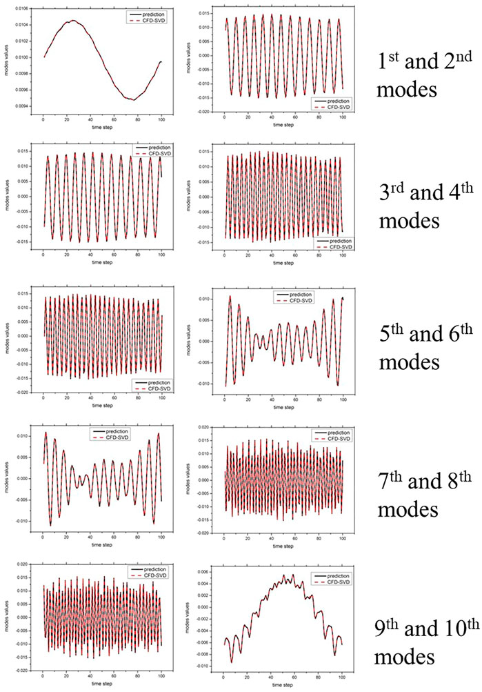
FIGURE 6. Comparison of first 10 orders of time coefficients between real and neural network prediction values. Black and red dotted lines represent time coefficients after reduced-order model prediction and computational fluid dynamics reduction, respectively.

Furthermore, the generalization of the neural network was analyzed, which indicated its adaptability to new samples. Adjusted R-square (AR²) was used for quantitative characterization. The value of AR² reflects the generalization performance of the ROM, that is, the degree of the ROM fitting to CFD data. The larger the value of AR², the better the fitting effect or prediction performance of the DNN. The mathematical expression for AR² is as follows:

${\mathit{R}}^2=1-\frac{{\sum }_{\mathit{i}=1}^{\mathit{n}}{\left({\mathit{u}}_{\mathit{i}}-{\widehat{\mathit{u}}}_{\mathit{i}}\right)}^2}{{\sum }_{\mathit{i}=1}^{\mathit{n}}{\left({\mathit{u}}_{\mathit{i}}-{\overline{\mathit{u}}}_{\mathit{i}}\right)}^2},(24)$

$\mathit{A}{\mathit{R}}^2=1-\frac{\left(1-{\mathit{R}}^2\right)\left(\mathit{n}-2\right)}{\mathit{n}-\mathit{p}-1},(25)$

where $u_i$ and ${\widehat{u}}_i$ are the predicted values and CFD, respectively, ${\overline{u}}_i$ is the average of the CFD results, n is the number of sampling points or the number of grid nodes, and p is the typical sample number or number of input parameters of the neural network. For the cylindrical flow in this study, p = 30. The AR² range distributions are presented in Table 1 and Figure 7. The AR² values of all time steps are >0.996, which indicates that the neural network model has a good generalization performance. The relative deviation of the ROM is <3%, which satisfies the requirements of engineering design applications.

TABLE 1

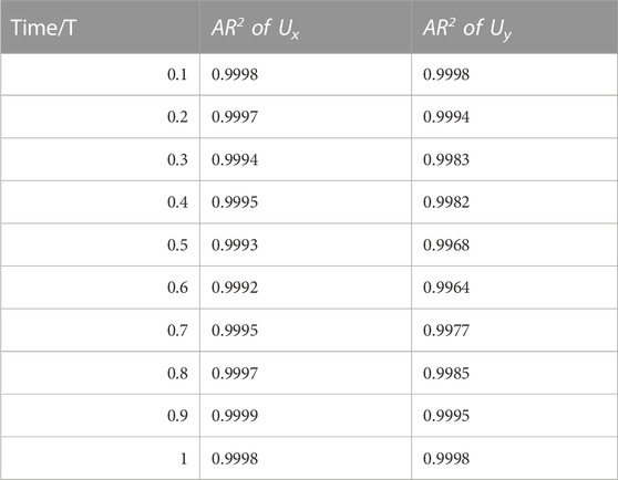
TABLE 1. AR² values of predicted results.

FIGURE 7

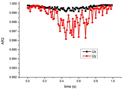
FIGURE 7. Distribution of AR² values with time step.

Table 2 summarizes CFD and ROM calculation times. After the acceleration of the graphics processing unit and completion of training, the ROM has to run for only a few seconds to generate the desired flow field variables. Under the existing grid scale, the speed of using the POD-DNN ROM is two orders of magnitude higher than that of the CFD numerical simulation, and it can easily predict the flow field variables at any moment, greatly reducing the calculation time and cost, and shortening the calculation cycle. It is noteworthy that sampling and training of data should be prepared prior to the ROM calculation.

TABLE 2

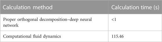
TABLE 2. Comparison of time consumption between full-order model (computational fluid dynamics) and reduced-order model.

3 Fast prediction of compressor three-dimensional flow field

The supercritical CO₂ centrifugal compressor is vital for the supercritical CO₂ Brayton cycle, which is the potential power cycle of the fourth generation nuclear power system. The supercritical CO₂ compressor has a compact structure, high efficiency, and broad application potential. It produces low temperature and low pressure CO₂, which completes the energy conversion through the blades driven by the motor and converts it into a high pressure gas, providing power for the supercritical CO₂ Brayton cycle. In the development of the nuclear power digital twin system, the compressor is the key component. Due to its huge consumption of numerical calculations, the real-time twinning operation of the compressor requires a faster calculation method. The POD-DNN in this study provides a feasible solution for the development of this digital twin.

3.1 Calculation object and establishment of POD-DNN flow field prediction model

The geometric model of the fluid domain of the supercritical CO₂ centrifugal compressor is shown in Figure 8. The number of grids used was 920,000. The variables to be predicted included density, pressure, and velocity in three directions, and the amount of data was 4.63 million. The data were obtained through CFD calculations using 22 different inlet temperature and flow combinations, of which 20 working conditions were used as the training sets and two were used as the test data.

FIGURE 8

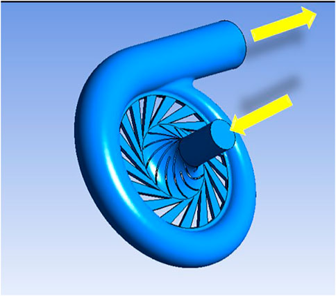
FIGURE 8. Compressor fluid domain model.

Owing to the large number and variety of flow field variables, a special incomplete neural network structure was designed in this study, which was classified into public and private layers, as shown in Figure 9. The public and private layer networks were fully connected, but the hidden and output layer neurons in the private layer network were partially connected. The private layer finally connects the specific output layer neuron to output specific variable results such as speed vector and pressure. In this way, the learning process of each layer parameter of the neural network was more targeted to provide a better fitting effect for the network.

FIGURE 9

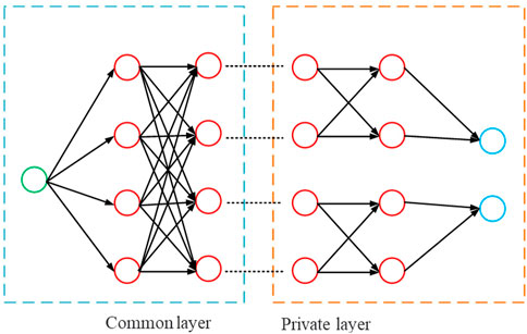
FIGURE 9. Incomplete neural network.

3.2 Results and discussion

Following the decomposition of POD, the relative deviation between the flow field reconstructed by POD and the original flow field after the 5th-, 10th-, and 15th-order truncations of each working condition is shown in Figure 10. It can be seen that with an increase in the POD truncation order, the relative deviation of POD reduction for each part of the flow fields is gradually reduced. Considering the large scale of data used for training, it is reasonable to use the 15-order truncation as the main mode for flow field reconstruction.

FIGURE 10

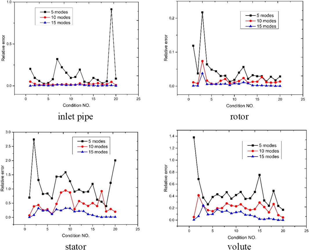
FIGURE 10. Comparison of reconstructed and original flow fields after POD truncation.

3.2.1 Results of velocity field prediction

Figures 11A, B show a comparison of the velocity cloud diagram between the POD-DNN and CFD on the z = 0 section. We have achieved rapid prediction of such a complex flow field based on deep learning for the first time. Previous research had primarily concentrated on simple two-dimensional flow or flow around a three-dimensional square cylinder, as was shown by Yousif (2022). The POD-DNN provides results that are consistent with the physical practice. The speed of the fluid rapidly increases as it enters the rotor, then it enters the diffuser, and gradually slows down before exiting through the volute. The highest speed found is in supercritical CO₂ at the rotor blade, which is slightly higher than the CFD result.

FIGURE 11

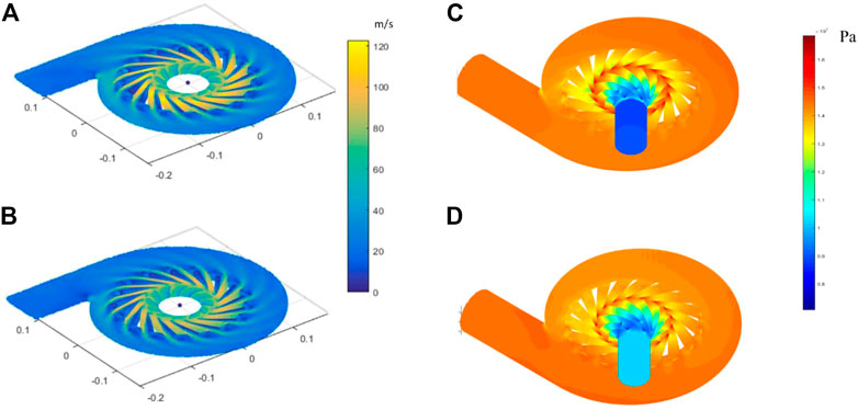
FIGURE 11. Comparisons of (A, B) velocity fields and (C, D) morphology of pressure fields. Certain differences between prediction results of POD–DNN (A, C) and results of calculation of computational fluid dynamics (B, D) in some areas are observed.

The relative deviation between the predicted value of the POD-DNN and the real value (CFD result) is defined as

$\mathit{\sigma }=\frac{\left|{\mathit{u}}_{\mathit{i}}-{\widehat{\mathit{u}}}_{\mathit{i}}\right|}{{\widehat{\mathit{u}}}_{\mathit{i}}}.(26)$

As shown in Figures 12A, 13A, through further quantitative analysis, the average relative deviation of the velocity prediction of 920,000 grid points is 9.7% and the prediction deviation of most grid points is within 15%. The velocity prediction error of the POD-DNN at the inlet pipe is approximately 30%, and the error in the rotor area is <10%. However, based on the distribution of the diffuser and volute, the prediction error of most grid points is <15%. When compared with the cylindrical flow around the cylinder, the POD-DNN significantly increases the deviation in predicting the compressor velocity field. Owing to the complexity of the flow field morphological structure, there is still a large deviation in the reconstructed flow field after the POD process, even though the 15th-order mode was adopted as the main mode of flow. A large reduction in the mode makes the training process more difficult, and the scale of data after dimensionality reduction affects the performance of the neural network. This result indicates that under this condition, the neural network training process may be trapped in a local optimum point.

FIGURE 12

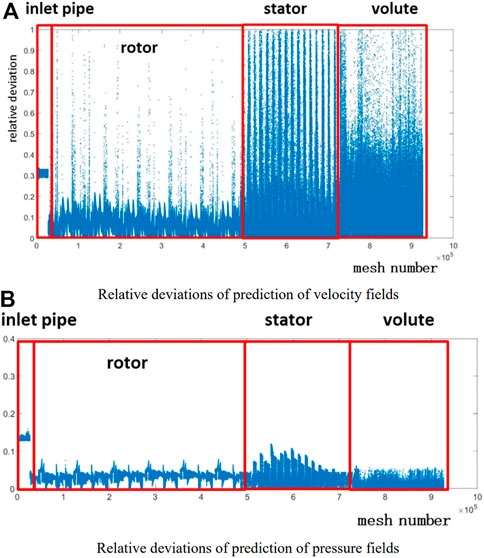
FIGURE 12. Scatter plots of relative deviations of prediction of (A) velocity and (B) pressure fields in each region.

FIGURE 13

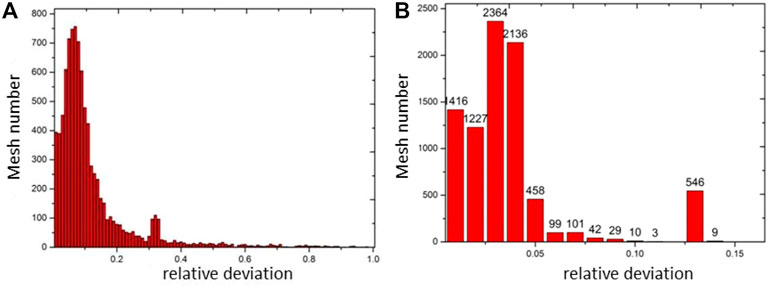
FIGURE 13. Relative deviations of prediction of (A) velocity and (B) pressure fields.

3.2.2 Results of pressure prediction

Figures 11C, D show a comparison of the pressure nephograms calculated using POD-DNN and CFD. It is observed that the pressure field results are similar, except for the inlet pipe. After supercritical CO₂ enters from the inlet pipe and passes through the rotor and diffuser, the pressure along the flow direction increases rapidly. The prediction of the internal pressure field is in accordance with the measured results.

Further quantitative analysis shows that the average relative deviation between the results of pressure field prediction and CFD is 3.05%, which significantly improved the accuracy of the prediction of pressure when compared with that of the velocity field. The pressure distribution was related to flow resistance and blade work pressurization, and it was smoother than that of the velocity field, suggesting that the prediction effect of the DNN was better. Figure 12B shows the predicted deviation of each calculation domain, and Figure 13B shows the columnar statistical distribution of the predicted relative deviation of the pressure field. It can be seen that the predicted deviation of the pressure value mainly originates from the inlet pipe and diffuser, and the deviation of the predicted pressure value relative to the true value reaches 13%.

In terms of generalization ability, the average relative deviation of the POD-DNN in the supercritical CO₂ compressor flow field prediction was <10%when compared with that of CFD. For the descending order of the compressor flow field, the characteristic number was p = 25 and the calibration determination coefficient was AR² = 0.9449. When compared with the surrounding cylindrical flow, three-dimensional flow field data of the compressor were large, flow characteristics were complex, and velocity and physical properties changed significantly. Therefore, the generalization ability of the neural network of the POD-DNN flow field prediction model of the compressor is not as good as that of the simple flow field of the surrounding two-dimensional flow. However, it plays a guiding role in the rapid design optimization of nuclear power systems and the determination of system operating conditions.

3.2.3 Prediction efficiency

In terms of the computational cost represented by the training time of the DNN, under the same computational resource configuration, the CFD calculation of each boundary condition took approximately 20 min, whereas the time spent on training the neural network was more than 6 h. However, the POD-DNN after training can provide modal coefficients in a few seconds and reconstruct the flow field, which takes <1% of the time required by CFD. This demonstrates that the presented model shows a remarkable reduction in the computational cost when compared to a full CFD simulation.

The POD-DNN used in this study is limited by resources and the performance of the server.

4 Conclusion

In this study, the feasibility of rapid flow field solutions in nuclear power system simulations, using model order-reduction technology based on DL, is discussed. A flow field prediction model based on POD and DNN was developed. The DNN was trained and tested using CFD data from the key flow equipment of the nuclear power system, and the prediction ability of the POD-DNN was verified.

For the compressor flow field prediction of key equipment in the nuclear power system, the first 15th-order POD modal coefficients were used for DNN training, and the average relative deviation between ROM and CFD was <10%. The verification results showed that the POD-DNN has the potential to predict large-scale complex flows. The ROM based on the POD-DNN framework can relatively extract the characteristics of the flow field accurately. Although the training time was long, and there was a gap between the predicted and actual results, the strong prediction ability and real-time simulation potential of flow field problems were reflected.

In a nuclear power system, the flow field of the core fuel assembly is the most complex and is a major cause of concern for researchers. The mesh number required for CFD simulation is as high as hundreds of millions or even billions, thereby restricting its use. The implementation of the POD-DNN in this study shows good utilization potential; however, it is necessary to further develop the order-reduction and prediction methods that can be applied to large-scale flow fields using big data technology in order to arrive at an efficient order-reducing algorithm that utilizes the deeper neural network model and reasonable sampling methods to ensure prediction accuracy with minimum samples.

Data availability statement

The raw data supporting the conclusion of this article will be made available by the authors, without undue reservation.

Author contributions

JY: software, methodology, and writing—original draft; DW: methodology; XS: methodology and supervision; YL: analysis; LZ: data curation; and YH: conceptualization, funding acquisition, and supervision. All authors contributed to the article and approved the submitted version.

Conflict of interest

The authors declare that the research was conducted in the absence of any commercial or financial relationships that could be construed as a potential conflict of interest.

Publisher’s note

All claims expressed in this article are solely those of the authors and do not necessarily represent those of their affiliated organizations, or those of the publisher, editors, and reviewers. Any product that may be evaluated in this article, or claim that may be made by its manufacturer, is not guaranteed or endorsed by the publisher.

Abbreviations

u₀, Average velocity; ${\phi }_n\left(x\right),$ eigenvector; $\lambda$, eigenvalue; $a_n\left(t\right),$ time coefficient; $\phi \left(z\right),$ activation function; $w_i$, weight; $b$, bias; $y_i$, prediction value; ${\widehat{y}}_i$, true value; $J\left(\theta \right)$, loss function; $g_t$, gradient of $J\left(\theta \right)$ with respect to θ under iterative step t; $m_t$, first-order momentum; ${\upsilon }_t$, second-order momentum; $\gamma$, contributions of previous gradients exponentially decaying; $\eta$, learning rate; ${\beta }_1$, exponential decaying rate of the first-order momentum; ${\beta }_2$, exponential decaying rate of the second-order momentum; $\sigma$, error of the velocity field obtained by the ROM; $U$, true velocity values matrix; $U_{ROM}$, prediction velocity values matrix; $R^2$, coefficient of determination; $A{R}^2$, adjusted coefficient of determination; ${\overline{u}}_i$, average of the true value; $n$, total number of samples; and $p$, number of features.

References

Bottou, L. (1998). “Online algorithms and stochastic approximations,” in Online learning in neural networks. Editor D. Saad (Cambridge, UK: Cambridge University Press).

Google Scholar

Bukka, S. R., Gupta, R., Magee, A. R., and Jaiman, R. K. (2021). Assessment of unsteady flow predictions using hybrid deep learning based reduced-order models. Phys. Fluids. 33, 013601. doi:10.1063/5.0030137

CrossRef Full Text | Google Scholar

Chen, D., Gao, X., Xu, C., Wang, S., Chen, S., Fang, J., et al. (2021). FlowDNN: A physics-informed deep neural network for fast and accurate flow prediction. Front. Inf. Technol. Electron. Eng. 23, 207–219. doi:10.1631/fitee.2000435

CrossRef Full Text | Google Scholar

Chen, X., Liu, L., Long, T., and Yue, Z. (2015). A reduced order aerothermodynamic modeling framework for hypersonic vehicles based on surrogate and POD. Chin. J. Aeronaut. 28, 1328–1342. doi:10.1016/j.cja.2015.06.024

CrossRef Full Text | Google Scholar

Chiekh, M. B., Michard, M., Guellouz, M. S., and Béra., J. C. (2013). Pod analysis of momentumless trailing edge wake using synthetic jet actuation. Exp.erimental Therm.al & Fluid Sci.ence 46, 89–102. doi:10.1016/j.expthermflusci.2012.11.024

CrossRef Full Text | Google Scholar

Chunyu, Z., Jiadong, W., Weilin, C., and Xiuqin, L. (2019). A fast solution method for parameterized high-fidelity models. Sci. China Phys. Mech. Astron. 49, 59–65. doi:10.1360/SSPMA2018-00286

CrossRef Full Text | Google Scholar

Glorot, X., Bordes, A., and Bengio, Y. Deep sparse rectifier neural networks. Proceedings of the 14th International Conference on Artificial Intelligence and Statistics (AISTATS), Fort Lauderdale, FL, USA, April 2011.

Google Scholar

Gupta, R., and Jaiman, R. (2022). Three-dimensional deep learning-based reduced order model for unsteady flow dynamics with variable Reynolds number. Phys. Fluids. 34, 033612. doi:10.1063/5.0082741

CrossRef Full Text | Google Scholar

Jarrett, K., Kavukcuoglu, K., Ranzato, M., and LeCun, Y. “What is the best multi-stage architecture for object recognition,” in Proceedings of the IEEE Proc. International Conference on Computer Visio, Kyoto, Japan, September 2009. doi:10.1109/ICCV.2009.54594692146一2153

CrossRef Full Text | Google Scholar

Kingma, D., and Ba, J. (2014). Adam: a method for stochastic optimization. Arxiv Preprint Arxiv, 1412.6980. doi:10.48550/arXiv.1412.6980

CrossRef Full Text | Google Scholar

Li, Y., Chang, J., Wang, Z., and Kong, C. (2021a). An efficient deep learning framework to reconstruct the flow field sequences of the supersonic cascade channel. Phys. Fluids. 33, 056106. doi:10.1063/5.0048170

CrossRef Full Text | Google Scholar

Li, Z. B., Wen, F. B., Tang, X., Su, L., and Wang, S. (2021). Prediction of single-row hole film cooling performance based on deep learning. Acta Aeronaut. Astronaut. Sin. 42, 12. doi:10.7527/S1000-6893.2020.24331

CrossRef Full Text | Google Scholar

Ling, J., Kurzawski, A., and Templeton, J. (2016). Reynolds averaged turbulence modelling using deep neural networks with embedded invariance. J. Fluid Mech. 807, 155–166. doi:10.1017/jfm.2016.615

CrossRef Full Text | Google Scholar

Marton, F., and Säaljö, R. (1976). On qualitative differences in learning-II: Outcome as a function of the learner’s conception of the task. Br. J. Educ. Psychol. 46, 115–127. doi:10.1111/j.2044-8279.1976.tb02304.x

CrossRef Full Text | Google Scholar

Maulik, R., San, O., Jacob, J. D., and Crick, C. (2019). Sub-grid scale model classification and blending through deep learning. J. Fluid Mech. 870, 784–812. doi:10.1017/jfm.2019.254

CrossRef Full Text | Google Scholar

Miyanawala, T. P., and Jaiman, R. K. (2017). An efficient deep learning technique for the Navier-Stokes equations: Application to unsteady wake flow dynamics. ArXiv Preprint. Arxiv. 1710. 09099. doi:10.48550/arXiv.1710.09099

CrossRef Full Text | Google Scholar

Morimoto, M., Fukami, K., and Fukagata, K. (2021). Experimental velocity data estimation for imperfect particle images using machine learning. Phys. Fluids. 33, 087121. doi:10.1063/5.0060760

CrossRef Full Text | Google Scholar

Nair, V., and Hinton, G. Rectified linear units improve restricted boltzmann machines. Proceedings of the 27th international conference on machine learning (ICML-10), Haifa Israel, June 2010.

Google Scholar

Rumelhart, D. E., Hinton, G. E., and Williams, R. J. (1986). Learning representations by back propagating errors. Nature 323 (6088), 533–536. doi:10.1038/323533a0

CrossRef Full Text | Google Scholar

San, O., and Maulik, R. (2018). Machine learning closures for model order reduction of thermal fluids. Appl. Math. Modell. 60, 681–710. doi:10.1016/j.apm.2018.03.037

CrossRef Full Text | Google Scholar

Schmid, P. J. (2010). Dynamic mode decomposition of numerical and experimental data. J. Fluid Mech. 656, 5–28. doi:10.1017/S0022112010001217

CrossRef Full Text | Google Scholar

Sekar, V., Jiang, Q., Shu, C., and Khoo, B. C. (2019). Fast flow field prediction over airfoils using deep learning approach. Phys. Fluids. 31, 057103. doi:10.1063/1.5094943

CrossRef Full Text | Google Scholar

Sirovich, L. (1987). Turbulence and the dynamics of coherent structures. I. Coherent structures. Quart. Appl. Math. 45, 561–571. doi:10.1090/qam/910462

CrossRef Full Text | Google Scholar

Taira, K., Hemati, M. S., Brunton, S. L., Sun, Y., Duraisamy, K., Bagheri, S., et al. (2020). Modal analysis of fluid flows: Applications and outlook. Aiaa J. 58, 998–1022. doi:10.2514/1.J058462

CrossRef Full Text | Google Scholar

Wilson, A. C., Roelofs, R., Stern, M., Srebro, N., and Recht, B. (2017). The marginal value of adaptive gradient methods in machine learning, Advances In Neural Information Processing Systems, 30, 08292. arXiv Preprint arXiv.1705. doi:10.48550/arXiv.1705.08292

CrossRef Full Text | Google Scholar

Xie, C., Yuan, Z., and Wang, J. (2020). Artificial neural network-based nonlinear algebraic models for large eddy simulation of turbulence. Phys. Fluids. 32, 115101. doi:10.1063/5.0025138

CrossRef Full Text | Google Scholar

Xinyu, H., Zelong, Y., and Junqiang, B. (2019). Prediction method of unsteady periodic flow based on deep learning. J. Aerodyn. 37, 462–469. doi:10.7638/kqdlxxb-2019.0003

CrossRef Full Text | Google Scholar

Yousif, M. Z., and Lim, H. C. (2022). Reduced-order modeling for turbulent wake of a finite wall-mounted square cylinder based on artificial neural network. Phys. Fluids 34, 015116. doi:10.1063/5.0077768

CrossRef Full Text | Google Scholar

Yuan, Z., Xie, C., and Wang, J. (2020). Deconvolutional artificial neural network models for large eddy simulation of turbulence. Phys. Fluids. 32, 115106. doi:10.1063/5.0027146

CrossRef Full Text | Google Scholar