Short-term load forecasting based on AM-CIF-LSTM method adopting transfer learning

Aiming at the unreliability of historical data for short-term load forecasting caused by the sudden change of power grid load under emergencies, a short-term load prediction method adopting transfer learning is studied. The proposed transfer learning method combines the attention mechanism (AM) with the long short-term memory network coupled with input and forgetting gates (CIF-LSTM) to construct the AM-CIF-LSTM short-term load prediction model. First, the variational modal decomposition (VMD) method is used to extract the trend component and certain periodic high-frequency components of the load datasets of the scene to be predicted and similar scenes. Subsequently, the AM-encoder/decoder learning model is established based on the trend component, and the AM learnable parameters are trained and transferred to the AM-CIF-LSTM model. Furthermore, inspired by the idea of classified forecasting, the load trend component and periodic high-frequency components under the required prediction scene are predicted by AM-CIF-LSTM and deep recursive neural network (DRNN), respectively. Finally, the load forecasting results are superimposed to obtain the load forecasting value. The experimental results demonstrate that the proposed method outperformed the existing methods in multiple accuracy indicators and could predict the rapid change trend of load in the case of insufficient data accurately and stably.

1 Introduction

Short-term load forecasting aims to calculate the electric load demand from hours to days in the future, which plays a very important role in the safe operation and optimal dispatching of modern power systems. In natural disasters, failures and other emergencies, the sudden change of power grid load will lead to unreliable historical load data, which greatly increases the difficulty of short-term load forecasting. Therefore, it is very important to design an accurate short-term load forecasting method to mitigate the impact of emergencies, which is a critical guarantee for power grid restoration and reconstruction and dispatching decision-making after the event.

The load in the modern power system has strong non-linearity and certain regularity. Various machine learning-based methods have been applied to load forecasting for their powerful non-linear processing capabilities by many scholars. These include support vector machines (Ma et al., 2019; Yang et al., 2019; Barman, Choudhury; Barman and Dev Choudhury, 2020), fuzzy logic (Rejc and Pantos, 2011), and artificial neural networks (Chen et al., 2010; Cecati et al., 2015). However, it is difficult for the traditional shallow machine learning models to fully capture the time series characteristics of load data, which affects the prediction accuracy. In recent years, deep learning methods have developed rapidly and gradually become the mainstream method for short-term load forecasting. Cai et al. (2019) used deep learning and conventional time-series techniques to compare the day-ahead load forecasting at the architectural level, and the results showed that the direct multi-step CNN model had the best prediction effect. Yang et al. (2020) employed probabilistic load prediction using Bayesian deep learning. Recurrent neural network (RNN) and its variants, such as deep recursive neural network (DRNN) (Chitalia et al., 2020), long short-term memory (LSTM) networks (Memarzadeh and Keynia, 2021; Peng et al., 2022), and gated recurrent units (Meng et al., 2022), have been widely used because they can deeply mine the time series characteristics of data and have high prediction accuracy.

However, the general deep learning method cannot accurately predict the rapid change trend of load after emergencies. On the one hand, emergencies greatly increase the non-stationary nature of load series. Although the deep learning models attributing to RNN have considered both the temporal and non-linear relationship of data, it is unable to make effective choices on a large number of temporal characteristics (Rodrigues and Pereira, 2020). On the other hand, deep learning models demand a large number of historical data, and sudden changes in power load caused by emergencies will lead to a decline in the reliability of historical load data, which will lead to the problem of overfitting. Migration learning can effectively solve the problem of insufficient training samples.

Transfer learning is a branch of the deep learning method (Tamaazousti et al., 2020). Its idea is to solve the task in the target domain by using the model trained in the source domain. It has been applied in medical, ecological, and other fields (Huynh et al., 2016; Li et al., 2017). In recent years, the results of transfer learning have also been gradually applied to power load forecasting (Cai et al., 2020; Gao et al., 2020; Zhou et al., 2020), which is a fresh idea to solve the lack of reliable historical data for short-term load forecasting.

Aiming at the mentioned difficulties of short-term load forecasting after encountering emergencies, the idea of transfer learning is introduced to establish the AM-CIF-LSTM model for short-term load forecasting in this paper. For the non-stationarity of load sequences, the variational mode decomposition (VMD) method is used to decompose it into a trend item and several periodic components. A transfer learning method based on the attention mechanism (AM) is established to solve the problem of unreliable historical data by training the learnable parameters in the attention model using the trend item of historical load data in similar scenes. To improve the computational efficiency, the long short-term memory network coupled with input and forgetting gates (CIF-LSTM) is constructed and the trained learnable parameters are transferred into it, which reduces the complexity of the traditional LSTM model and relieves the huge computational burden brought by transfer learning. CIF-LSTM and DRNN are employed to predict trend items and high-frequency periodic components respectively, and the final prediction result is obtained by superposing the above two parts of predicted values. Finally, the case study is implemented to verify the accuracy of the proposed method in forecasting rapidly changing loads, the effectiveness to solve historical data lack problem.

2 Transfer learning method based on AM

In the proposed AM-based transfer learning method, the inputs and outputs of the training model are the load trend items decomposed by the VMD, and the migration object is the learnable parameter in AM and encoder-decoder structure.

2.1 VMD

The power load can be divided into two parts. One is a low-frequency basic load, corresponding to the fixed basic load in production and life. The other is several high-frequency floating loads with different cycles, which are relatively stable and may correspond to different forms of human life and production electricity (Zhang et al., 2021). It can be considered that the changing trend of the lowest frequency sequence obtained from the power load decomposition can represent significant changes in the system.

To avoid over-decomposition and mode mixing, VMD is used to decompose the load sequence. VMD is a completely non-recursive signal decomposition method (Dragomiretskiy and Zosso, 2014), which assumes that any signal is composed of a finite number of bandwidth intrinsic mode functions (BIMFs) with a specific center frequency and limited bandwidth (Junsheng et al., 2006). Given modal number K and penalty factor α, the original signal L(t) can be adaptively decomposed into K BIMFs by constraining that the total bandwidth of the center frequencies of each modal component is minimum and the sum of all modal components are equal to the original signal. The basic steps of decomposition are as follows.

(1) For the i-th modal component m_i(t), perform Hilbert transform to obtain its analytical signal and unilateral spectrum, and modulate the spectrum of the analytical signal to the fundamental frequency band corresponding to the estimated central frequency by adding the exponential term $e^{-j{\omega }_{i}t}$:

$\left[\left(\delta \left(t\right)+\frac{j}{\pi t}\right)*m_i\left(t\right)\right]e^{-j{\omega }_{i}t}(1)$

where $\delta \left(t\right)$ is Dirac distribution; * represents convolution operation; j is an imaginary number; t is the sampling time.

(2) Calculate the estimated bandwidth of each modal signal by the L2 norm of the demodulated signal gradient. The corresponding constrained variational model is as follows

$\left\{\begin{array}{l}\underset{\left\{m_i\right\},\left\{{\omega }_i\right\}}{\min }\left\{{\displaystyle \sum }_{i=1}^N{‖{\partial }_t\left[\left(\delta \left(t\right)+\frac{j}{\pi t}\right)*m_i\left(t\right)\right]e^{-j{\omega }_{i}t}‖}_2^2\right\}\\ \mathrm{s}.\mathrm{t}.{\displaystyle \sum }_{i=1}^N{m}_i\left(t\right)=L\left(t\right)\end{array}\right.(2)$

where $\left\{m_i\right\}=\left\{m_1,m_2,\dots ,m_N\right\}$ is the modal component; $\left\{{\omega }_i\right\}=\left\{{\omega }_1,{\omega }_2,\dots ,{\omega }_N\right\}$ is the frequency center of each component.

(3) By introducing Lagrange Multiplier $\lambda \left(t\right)$ and penalty factor α, transformed the constrained variational problem into the following unconstrained variational model:

$\begin{array}{l}\mathcal{l}\left(m_i,{\omega }_i,\lambda \right)=\alpha {\displaystyle \sum }_{i=1}^N{‖{\partial }_t\left[\left(\delta \left(t\right)+\frac{j}{\pi t}\right)*m_i\left(t\right)\right]e^{-j{\omega }_{i}t}‖}_2^2\\ +{‖L\left(t\right)-{\displaystyle \sum }_{i=1}^N{m}_i\left(t\right)‖}_2^2\\ +〈\lambda \left(t\right),L\left(t\right)-{\displaystyle \sum }_{i=1}^N{m}_i\left(t\right)〉\end{array}(3)$

(4) Solve the above equation using the Alternating Direction Method of Multipliers. The update formula of {m_i} and {ω_i} as follows:

$\left\{\begin{array}{l}{\widehat{m}}_i^{k+1}\left(\omega \right)=\frac{\widehat{L}\left(\omega \right)-\sum _{p\ne i}^N{\widehat{m}}_p^k\left(\omega \right)+\frac{{\widehat{\lambda }}^k\left(\omega \right)}{2}}{1+2\alpha {\left(\omega -{\omega }_i^k\right)}^2}\\ {\omega }_i^{k+1}=\frac{{{\int }_0^{\infty }\omega \left|{\widehat{m}}_i^{k+1}\left(\omega \right)\right|}^{2}d\omega }{{{\int }_0^{\infty }\left|{\widehat{m}}_i^{k+1}\left(\omega \right)\right|}^{2}d\omega }\end{array}\right.(4)$

where ${\widehat{m}}_i^{k+1}\left(\omega \right)$, $\widehat{L}\left(\omega \right)$, and ${\widehat{\lambda }}^k\left(\omega \right)$ are respectively the Fourier transforms of $m_i^{k+1}\left(t\right)$, $L\left(t\right)$, and ${\lambda }^k\left(t\right)$; k is the number of iterations. When Eq. 5 is established, the iteration stops and the final modal component is obtained.

${\displaystyle \sum }_{i=1}^N\frac{{‖m_i^{k+1}-m_i^k‖}_2^2}{{‖m_i^k‖}_2^2}<\eta (5)$

2.2 AM

As a resource allocation scheme, the AM uses limited computing resources to process more important information, which is the main means to address information overload. The AM was mostly used in natural language processing (Bahdanau et al., 2016), and it has been favored in several forecasting problems (Qin et al., 2017; Chen et al., 2018).

Since transfer learning requires a large amount of source data for learnable parameters training, and information at different times has different influence on the load at the predicted time, AM is introduced to improve the information processing ability of the neural networks, so as to reduce the computational burden.

The basic structure of AM is shown in Figure 1. Information is filtered through the following two steps: 1) Calculating the attention distribution on all input information; 2) Calculating the weighted average of the input information according to the attention distribution.

FIGURE 1

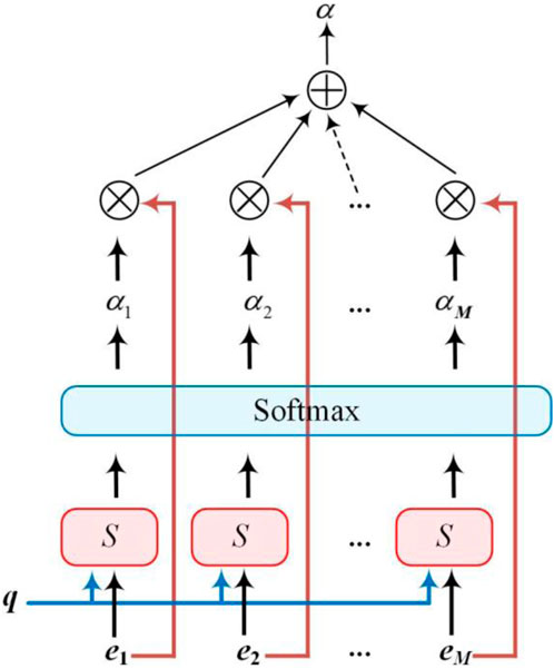
FIGURE 1. Basic structure of AM.

To select information related to a specific task from M input vectors, $E=\left(e\_\left(1\right),e\_\left(2\right),\dots ,e\_\left(M\right)\right)$, we should introduce a task-related representation, called a query vector, and calculate the correlation between each input vector and query vector through a scoring function. Given a task-related query vector q, the query vector q can be dynamically generated or a learnable parameter. In this study, we use q as a learnable parameter to implement transfer learning.

The attention variable is used to represent the index position of the selected information. First, we calculate the probability α_i of selecting the i-th input vector under given q and E:

$\begin{array}{l}{\alpha }_i=soft\max (s(e_i,q)\\ =\frac{\exp \left(s\left(e_i,q\right)\right)}{{\displaystyle \sum }_{i=1}^M\exp \left(s\left(e_i,q\right)\right)}\end{array}(6)$

where α_i is the attention distribution and can be interpreted as the degree of attention to the i-th input vector when the task-related query q is given, and s(e,q) is the attention scoring function, whose dot product form is:

$s\left(e,q\right)=e^{\mathrm{T}}q(7)$

Then, the output vector of AM is obtained by weighting the input vectors using α_i, which is calculated as follows:

$\mathrm{a}\mathrm{t}\mathrm{t}\left(E,q\right)={\displaystyle \sum }_{i=1}^M{\alpha }_i{e}_i(8)$

where att(E,q) is the information obtained according to the attention distribution and denotes the expectation of all input vectors $\left(e_1,e_2,\dots ,e_M\right)$ under the attention distribution.

The attention mechanism can be used independently, but more often, it is used as a component of the neural network. In this study, we used it as a tool for transfer learning and connected it to the encoder−decoder and CIF-LSTM network. The implementation steps can be summarized as: 1) extract the trend items of the source load sequence using VMD, 2) divide this trend term into several sequences in time order, with the preceding sequences as the Encoder inputs and the subsequent sequence as the Decoder input, to train the learnable parameters in the AM, and 3) embed the trained learnable parameters into the AM of the new prediction model, and take the output of AM as the input of CIF-LSTM.

3 AM-CIF-LSTM forecasting model based on transfer learning

3.1 CIF-LSTM network

The introduction of transfer learning and classified forecasting can theoretically improve the short-term load forecasting accuracy after emergencies, but it also brings a large source data set and the amount of computation that increases exponentially with the number of load decompositions. LSTM is a variant of RNN. It not only solves the gradient disappearance problem of RNN (Hochreiter and Schmidhuber, 1997) but also reduces the dependence on information length. LSTM has great advantages in processing sequence data but a large amount of computation. Therefore, it is necessary to use a simplified LSTM recurrent unit to minimize the computation while maintaining its performance.

3.1.1 LSTM network

In the LSTM network, a new internal state c_t is introduced for linear circular information transmission, and the information is non-linearly output to the external state h_t of the hidden layer. The internal state c_t is calculated as:

$c_t=f_t\odot c_{t-1}+i_t\odot {\stackrel{\sim }{c}}_t(9)$

$h_t=o_t\odot \tanh \left(c_t\right)(10)$

where ⊙ represents the product of vector elements; c_t-1 is the internal memory state of the previous moment; ${\stackrel{\sim }{c}}_t=\tanh \left(W_c{x}_t+U_c{h}_{t-1}+b_c\right)$ is the state to be output; i_t is the input gate, which controls the state to be output at the current time and the information to be saved for each input; f_t is the forgetting gate, which controls the information that should be forgotten in the last internal memory state c_t-1; o_t is the output gate, which controls the internal memory state c_t that must be output to the external state h_t of the hidden layer.

The calculation method for the three gates is as follows.

$i_t=\sigma \left(W_i{x}_t+U_i{h}_{t-1}+b_i\right)(11)$

$f_t=\sigma \left(W_f{x}_t+U_f{h}_{t-1}+b_f\right)(12)$

$o_t=\sigma \left(W_o{x}_t+U_o{h}_{t-1}+b_o\right)(13)$

where σ is the logistic function with the output interval of (0,1); x_t is the input information of the t-th iteration; h_t-1 is the external state of the t-1-th iteration.

3.1.2 CIF-LSTM network

Jozefowicz et al. (2015) evaluated more than 10,000 RNN architectures and found that adding bias term one to the forgetting gate of LSTM improves its performance. Greff et al. (2017) tested Several variants of LSTM and, it was concluded that simplifying certain structures of LSTM can effectively improve the computational efficiency without affecting the performance.

To improve the calculation efficiency, this study draws on the conclusions of the former two and adopts CIF-LSTM. The basic unit structure of the network is shown in Figure 2. The improved forgetting gate is calculated as:

$f_t=1-i_t(14)$

FIGURE 2

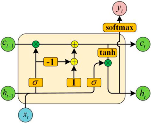
FIGURE 2. Basic unit structure diagram of CIF-LSTM network.

As shown in Figure 2, the characteristic of this variant cell is the replacement of the forgetting gate with the negative value of the input gate plus a bias term 1. That greatly reduces the operation of the forgetting gate by replacing the previous logic function containing exponential operations and multiplication and division operations with simple addition and subtraction operations, thus alleviating the computational burden caused by migration learning.

3.2 Framework of the proposed forecasting model

The AM-CIF-LSTM load forecasting model based on transfer learning proposed in this paper consists of transfer learning and load forecasting. The model framework is shown in Figure 3.

FIGURE 3

FIGURE 3. Framework of the proposed load forecasting model.

In the part of migration learning, VMD is used to decompose dataset I under similar scenarios and obtain its trend component. Then, based on the encoder-decoder structure, the learnable parameters of the AM are trained through the trend items. Then, the learnable parameters are embedded into the AM-CIF-LSTM network of the load forecasting part to realize transfer learning.

In the part of load forecasting, the network needs to be trained on the training set firstly. The model hyperparameters are determined by the verification set. When forecasting on the test set, the historical load sequences of the area to be predicted is decomposed into a trend item and several high-frequency periodic components by VMD. For the trend item, the AM with learnable parameters is used to weight the load segment, and then the trained CIF-LSTM network is used to predict it. For high-frequency periodic components, the trained DRNN is used for prediction. Finally, the predicted value of the load can be obtained by superposition of the results.

3.3 Solution of the forecasting model

3.3.1 Measurement method of data set similarity

To achieve accurate load prediction under different scenarios, it is necessary to extract load sequences similar to the scenarios of the load to be predicted from the source data set for transfer learning. Therefore, after obtaining the load trend item sequences using VMD, it is necessary to measure its similarity with the load sequence of the source dataset. In fact, the regularity of the historical load sequences after the emergency is strong, but the regularity of the external factor data causing the load sudden change, such as meteorological data and fault data, is poor (Liu et al., 2014).

Therefore, considering the data distribution and the morphological fluctuation characteristics of the load trend items, the dynamic time warping (DTW) distance is employed to measure the similarity of the load sequences. According to the similarity, the data set is divided into different scenes using the interquartile range judgment criterion to realize the scene classification of different historical load curves. The implementation steps are as follows.

(1) Calculate the DTW distance between the load sequences of the source dataset and the load sequences to be predicted.

DTW obtains the optimal curve path by adjusting the relationship between the corresponding elements at different time points in the time series and measures their similarity by the optimal path distance.

For two given time series $X=\left(x_1,x_2,\dots ,x_n\right)$ and $R=\left(r_1,r_2,\dots ,r_m\right)$, an n×m distance matrix D_n×m is constructed, whose element D(i,j) is the Euclidean distance between x_i and r_j and calculated as

$D\left(i,j\right)=\sqrt{{\left(x_i-r_j\right)}^2}(15)$

The set of each group of adjacent elements in the matrix D is called a curved path, and it needs to meet the constraints of boundary, continuity and monotonicity, denoted as p = {p₁, p₂, …, p_s, …, p_k}, Where k is the total number of elements in the path, and the element p_s is the coordinate of the s-th point on the path, that is, p_s = (i, j).

The optimal curve path distance between X and Y, namely DTW distance, is calculated as

$\mathrm{D}\mathrm{T}\mathrm{W}\left(X,Y\right)=L\left(i,j\right)=D\left(i,j\right)+\min \left\{L\left(i-1,j-1\right),L\left(i,j-1\right),L\left(i-1,j\right)\right\}(16)$

(2) Based on the calculated DTW distance, the quartile distance criterion is used to eliminate the load sequences with low similarity, to select the historical load dataset in the same scenario.

3.3.2 Hyperparameter optimization

The AM-CIF-LSTM prediction framework based on transfer learning proposed in this paper is a very large multi-prediction model. A large number of hyperparameters need to be configured for prediction processes. Therefore, the hyperparameters should be optimized to reduce the computational burden.

Since the current optimization methods of neural networks generally adopt stochastic gradient descent, we can use the learning curve of a set of hyperparameters to estimate whether this set of hyperparameter configurations is hopeful of obtaining better results. If the learning curve of a set of hyperparameter configurations does not converge or the convergence is poor, an early-stopping strategy can be applied to terminate the current training, so as to leave resources to other hyperparameter configurations.

To effectively find the optimal hyperparameters of each prediction model, improve the final prediction accuracy, and ensure the feasibility of the model, the successive halving method is applied for dynamic resource allocation. This method regards the hyperparameter optimization as a non-random optimal arm problem. Assuming that N sets of hyperparameter configurations are to be tried, the total available resource budget is B, the optimal hyperparameter configuration group can be selected through T =log2(N)-1 round of halving calculation. The algorithm is shown in Table 1.

TABLE 1

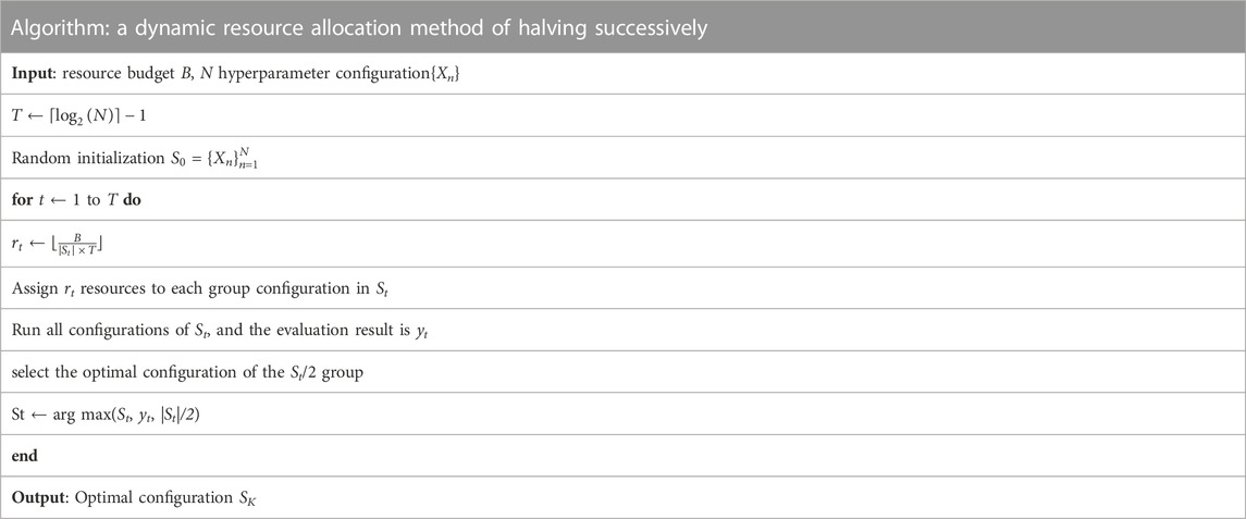
TABLE 1. Successive halving algorithm.

3.3.3 Solution steps

The solution process of the proposed short-term load forecasting model is shown in Figure 4.

FIGURE 4

FIGURE 4. Flow chart of solving steps for the proposed load forecasting model.

The basic steps are summarized as follows:

Step 1:. Data partitioning and preprocessing. The original data are collect and divided into source data set (data set O) for migration learning and data set II for load forecasting, and deal with missing and invalid values.

Step 2:. Load decomposition. VMD is used to extract the trend items and high-frequency periodic components of the source dataset and dataset I.

Step 3:. Data set similarity measurement. Based on Eq. 20, the source dataset is classified by the trend items, and the historical load with the highest similarity to the trend items of data set II is selected as data set I, which is used as the migration learning training data of data set II;

Step 4:. Transfer learning. The learning model based on AM encoder/decoder is established, and the learnable parameters of the model are trained using the load trend items of dataset I;

Step 5:. Load forecasting. The learnable parameters are migrated to the AM-CIF-LSTM model to predict the trend items of dataset II, and the other periodic high-frequency components of dataset II are predicted using DRNN.

Step 6:. Add the predicted results in step 5 to obtain the final predicted value.

4 Case study

4.1 Example system

In this study, we selected the historical load of a region from 2013 to 2015 as the original data, which is divided into the source data set used for migration learning (70%) and the data set II used for load forecasting (30%). 50% of the data in dataset II was divided into training sets for training neural networks. The remaining data are equally divided into verification set and test set, which are respectively used to determine the super parameters and test the prediction effect. The sampling interval of each load data section is 1 h, and there are 350-time sampling points in total.

Simulations were implemented in a MATLAB environment on an Intel Core i5-4590 CPU with a 3.30-GHz, 12.0-GB RAM personal computer.

4.2 Data preprocessing

After data collection, the missing or invalid values of the original data were processed firstly. To address the data loss or bad data caused by certain objective factors, the linear interpolation method is used to fill the corresponding data, as shown in the following formula.

${x_t}^{\prime }=\frac{x_{t+s}-x_{t-s}}{2}(17)$

where ${x_t}^{\prime }$ is the interpolation value of missing data, and its order in all sample data sets is t; s is the distance between the reference data and the missing data, which is the distance between the data to be filled and the nearest available data.

4.3 Evaluation metrics

To measure the performance of the load forecasting method, four indicators were adopted in this study, including mean absolute error (MAE), root mean square error (RMSE), means absolute percentage error (MAPE) and forecasting accuracy (FA).

The smaller the value of MAE, RMSE and MAPE, and the larger the value of FA, the closer the predicted value is to the observed value, namely, the better the performance of the prediction method. The above indicators are calculated by Eqs 18–21 respectively:

$MAE=\frac{1}{N}{\displaystyle \sum }_{j=1}^n\left|y_j-y_j^{\prime }\right|(18)$

$RMSE=\sqrt{\frac{1}{N}{\displaystyle \sum }_{j=1}^n{\left(y_j-y_j^{\prime }\right)}^2}(19)$

$MAPE=\frac{1}{N}{\displaystyle \sum }_{j=1}^n\frac{\left|y_j-y_j^{\prime }\right|}{y_j}*100(20)$

$FA=\frac{1}{N}{\displaystyle \sum }_{j=1}^n\left(1-\frac{\left|y_j-y_j^{\prime }\right|}{y_j}\right)*100\%(21)$

where: y_j is the true load value of the j-th sampling point; $y_j^{\prime }$ is the load forecast value of the j-th sampling point; $\overline{y}$ is the mean value of the true load value; $\overline{y^{\prime }}$ is the mean value of the load forecast value; N is the number of elements in the dataset.

4.4 VMD results

The modal decomposition number and the penalty factor value are important factors affecting the VMD decomposition performance. To avoid the subjectivity of empirical selection methods, the energy difference principle (Junsheng et al., 2006) is introduced to determine its parameters. According to the calculation results, K is set to 6, penalty factor is set to 1999, Tolerance is set to 10-6. Figure 5 shows the six rapidly changing load sections in the training set and their VMD decomposition results.

FIGURE 5

FIGURE 5. VMD results.

As can be seen from Figure 5, the original load sequences are decomposed into five high-frequency periodic components, BIMF1∼BIMF5, and a trend item, res. The frequencies of these periodic components are relatively concentrated and non-aliased, which reflect periodic factors that affect the load changes. So that the periodic components can be regarded as stationary sequences. Considering their efficiency and performance, these components are suitable for prediction using DRNNs (Meng et al., 2022). After separately forecasting and superimposing the components, the high-frequency part of the load forecast result is obtained.

The figure also shows that, after removing the high-frequency components from the load curve, a relatively flat load trend curve is obtained. It reflects the changes in the baseline value of the load, and it physically corresponds to the emergency scene considered for this study.

It can be seen from the above analysis that the seemingly chaotic conventional load sequence can be decomposed into several high-frequency components with different periods and a trend item. Extracting the load trend item for forecasting can weaken the interference of high-frequency components and effectively identify the impact of emergencies on load.

4.5 Load forecast results

From the test set, the load series of the rapidly changing reduction section and recovery section were extracted to show the prediction effect. To analyze the accuracy of the short-term load forecasting method proposed in this paper, three forecasting methods are set for comparison, and the data sets used to train the models are the same for all methods.

Method 1: DRNN.

Method 2: Deep LSTM network (DLSTMN).

Method 3: The proposed method (PM), namely AM-CIF-LSTM based on transfer learning.

Figures 6A,B show the forecasting results of the load reduction section and the load recovery section under different methods respectively.

FIGURE 6

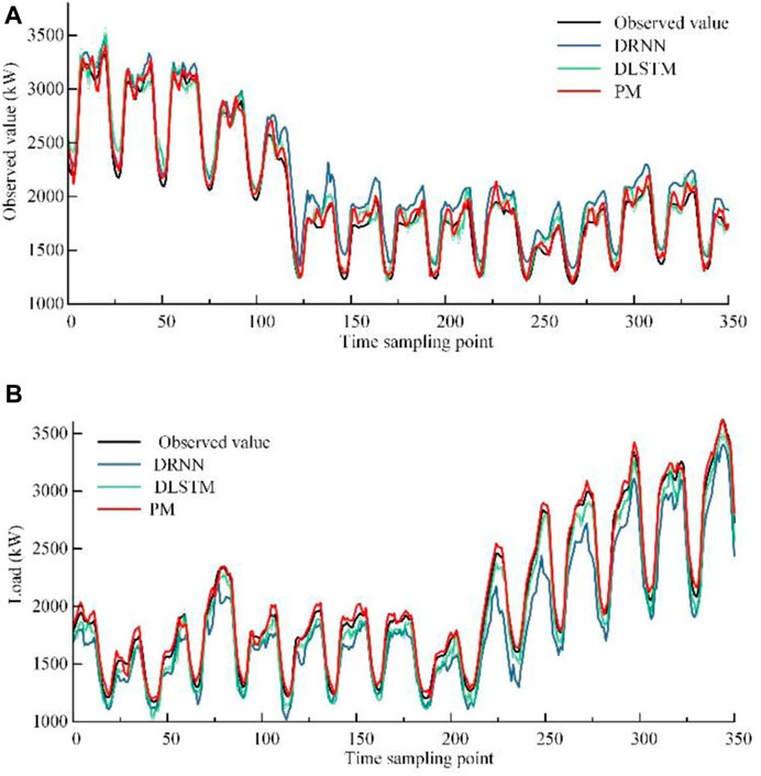
FIGURE 6. Comparison of load prediction results. (A) Load forecasting results in the load recovery section. (B) Load forecast results in the load recovery section.

It can be seen from Figure 6A that the load is in a downward trend between the 100th and 125th sampling times. From Figure 6B, it can be observed that the load trend is on the rise between the 200th and 325th sampling times. The non-stationary of the load sequence increased significantly during the reduction or recovery period.

By comparing the predicted load curves of DRNN and DLSTM during load changes in Figures 6A,B, respectively, it can be found that when the load sequences is relatively regular, the predicting performance of DRNN and DLSTM is similar. However, when load trend change rapidly, the forecasting accuracy of DLSTM is higher, and the forecasting accuracy of DRNN is reduced significantly. That indicates that DRNN can achieve accurate prediction with a simple structure for more regular load sequences, and DLSTM has the advantages in processing long time sequences by better use historical data.

Comparing the predicted load curve obtained by the three methods in Figures 6A,B with the observed load, it can be observed that the predicted load curve obtained by PM is closer to the observed load curve than that obtained by DRNN and DLSTM, no matter in the process of rapid load change or before and after the change. This indicates that employing the AM-CIF-LSTM based on migration learning to predict the trend items can improve the prediction accuracy when the load trend changes significantly, which solves the problem of insufficient historical load data under emergencies. Using DRNN to predict high-frequency components can ensure the prediction accuracy of relatively stable periodic components while reducing the computational burden.

To quantitatively analyze and comprehensively compare the load forecasting performance of DRNN, DLSTMN, and PM, four evaluation indicators of load forecasting results under the three methods are calculated respectively, as shown in Table 2.

TABLE 2

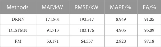
TABLE 2. Comparison of indicators of different methods.

As shown in Table 2, compared with DRNN and DLSTMN, the MAE of PM decreases by 69.05% and 42.03% respectively; RMSE decreases by 66.64% and 37.43% respectively; MAPE decreases by 68.46% and 42.52% respectively; FA increased by 6.73% and 2.19% respectively. That indicates that the overall prediction error of PM is smaller and the prediction accuracy is higher.

According to the above analysis, in the case of sudden load changes, the proposed method can solve the problem of limited reliable historical load data by introducing migration learning and classification prediction. Compared with other methods, the prediction accuracy has been greatly improved.

5 Conclusion

To accurately predict the load trend under emergencies, an AM-CIF-LSTM short-term load forecasting method based on transfer learning is proposed in this paper, and its effectiveness is verified by the case study. The characteristics of the proposed method are concluded as follows:

1) Aiming at the shortage of reliable historical load data and the consequent overfitting problem, a transfer learning method based on AM is proposed. The learning and utilization of similar historical data are realized just by the encoder-decoder structure and attention model, which solves the invalidity of traditional methods in such applications.

2) To improve the forecasting accuracy under the circumstances that the load suddenly changes, the idea of classified forecasting is introduced. The load is decomposed into a trend item and several high-frequency periodic components using VMD. The AM training by the transfer learning training is combined with CIF-LSTM to predict the trend items, and DRNN is utilized to predict the high-frequency periodic components, which effectively improves the prediction accuracy by reducing the non-stationary load sequences.

3) To improve the calculation efficiency of load forecasting, a CIF-LSTM network is proposed by coupling the input gate and forgetting gate of the traditional LSTM basic unit. The computational complexity is reduced by simplifying the network structure, and the computational efficiency is improved without affecting the accuracy.

The short-term load forecasting method proposed in this study is developed based on point prediction. If load forecasting is conducted by interval forecasting and even probability forecasting, the obtained prediction results would contain more information, which is conducive for decision-makers to make more reasonable planning and scheduling plans for power systems.

Data availability statement

The original contributions presented in the study are included in the article/supplementary materials, further inquiries can be directed to the corresponding authors.

Author contributions

SL and XW contributed to conception and design of the study. XW and BX organized the database. SL and LY conducted the simulation verification. SL wrote the first draft of the manuscript, which was reviewed and edited by LY and HW. All authors agree to be accountable for the content of the work.

Funding

This work is supported by the Science and Technology Major Projects of Anhui Province under Grant 202203f07020003.

Conflict of interest

Authors XW and BX were employed by State Grid Anhui Electric Power Research Institute.

The remaining authors declare that the research was conducted in the absence of any commercial or financial relationships that could be construed as a potential conflict of interest.

Publisher’s note

All claims expressed in this article are solely those of the authors and do not necessarily represent those of their affiliated organizations, or those of the publisher, the editors and the reviewers. Any product that may be evaluated in this article, or claim that may be made by its manufacturer, is not guaranteed or endorsed by the publisher.

References

Bahdanau, D., Chorowski, J., Serdyuk, D., Brakel, P., and Bengio, Y. “End-to-end attention-based large vocabulary speech recognition,” in Proceedings of the 2016 IEEE International Conference on Acoustics, Speech and Signal Processing (ICASSP), Shanghai, China, March 2016 (Shanghai: Speech Signal Process.), 4945–4949.

Google Scholar

Barman, M., and Choudhury, N. B. D. (2019). Season specific approach for short-term load forecasting based on hybrid FA-SVM and similarity concept. Energy 174, 886–896. doi:10.1016/j.energy.2019.03.010

CrossRef Full Text | Google Scholar

Barman, M., and Dev Choudhury, N. B. (2020). A similarity based hybrid GWO-SVM method of power system load forecasting for regional special event days in anomalous load situations in Assam, India. Sustain. Cities Soc. 61, 102311. doi:10.1016/j.scs.2020.102311

CrossRef Full Text | Google Scholar

Cai, L., Gu, J., and Jin, Z. (2020). Two-layer transfer-learning-based architecture for short-term load forecasting. IEEE Trans. Ind. Inf. 16 (3), 1722–1732. doi:10.1109/tii.2019.2924326

CrossRef Full Text | Google Scholar

Cai, M., Pipattanasomporn, M., and Rahman, S. (2019). Day-ahead building-level load forecasts using deep learning vs. traditional time-series techniques. Appl. Energy 236, 1078–1088. doi:10.1016/j.apenergy.2018.12.042

CrossRef Full Text | Google Scholar

Cecati, C., Kolbusz, J., Ró˙zycki, P., Siano, P., and Wilamowski, B. M. (2015). A novel RBF training algorithm for short-term electric load forecasting and comparative studies. IEEE Trans. Ind. Electron. 62 (10), 6519–6529. doi:10.1109/tie.2015.2424399

CrossRef Full Text | Google Scholar

Chen, T., Yin, H., Chen, H., Wu, L., Wang, H., Li, X., et al. (2018). Tada: Trend alignment with dual-attention multi-task recurrent neural networks for sales prediction. Proc. ICDM, 49–58.

CrossRef Full Text | Google Scholar

Chen, Y., Luh, P. B., Guan, C., Zhao, Y., Michel, L. D., Coolbeth, M. A., et al. (2010). Short-term load forecasting: Similar day-based wavelet neural networks. IEEE Trans. Power Syst. 25 (1), 322–330. doi:10.1109/tpwrs.2009.2030426

CrossRef Full Text | Google Scholar

Chitalia, G., Pipattanasomporn, M., Garg, V., and Rahman, S. (2020). Robust short-term electrical load forecasting framework for commercial buildings using deep recurrent neural networks. Appl. Energy 278, 115410. doi:10.1016/j.apenergy.2020.115410

CrossRef Full Text | Google Scholar

Dragomiretskiy, K., and Zosso, D. (2014). Variational mode decomposition. IEEE Trans. Signal Process. 62 (3), 531–544. doi:10.1109/TSP.2013.2288675

CrossRef Full Text | Google Scholar

Gao, Y., Ruan, Y., Fang, C., and Yin, S. (2020). Deep learning and transfer learning models of energy consumption forecasting for a building with poor information data. Energy Build. 223, 110156. doi:10.1016/j.enbuild.2020.110156

CrossRef Full Text | Google Scholar

Greff, K., Srivastava, R. K., Koutník, J., Steunebrink, B. R., and Schmidhuber, J. (2017). Lstm: A search space odyssey. IEEE Trans. Neural Netw. Learn. Syst. 28 (10), 2222–2232. doi:10.1109/tnnls.2016.2582924

PubMed Abstract | CrossRef Full Text | Google Scholar

Hochreiter, S., and Schmidhuber, J. (1997). Long short-term memory. Neural comput. 9 (8), 1735–1780. doi:10.1162/neco.1997.9.8.1735

PubMed Abstract | CrossRef Full Text | Google Scholar

Huynh, B., Drukker, K., and Giger, M. (2016). MO-DE-207B-06: Computer-Aided diagnosis of breast ultrasound images using transfer learning from deep convolutional neural networks. Med. Phys. 43 (6), 3705. doi:10.1118/1.4957255

CrossRef Full Text | Google Scholar

Jozefowicz, R., Zaremba, W., and Sutskever, I. “An empirical exploration of recurrent network architectures,” in Proceedings of the 32nd International Conference on International Conference on Machine Learning, Lille, France, July 2015.

Google Scholar

Junsheng, C., Dejie, Y., and Yu, Y. (2006). Research on the intrinsic mode function (IMF) criterion in EMD method. Mech. Syst. Signal Process. 20 (4), 817–824. doi:10.1016/j.ymssp.2005.09.011

CrossRef Full Text | Google Scholar

Li, N., Hao, H., Gu, Q., Wang, D., and Hu, X. (2017). A transfer learning method for automatic identification of sandstone microscopic images. Comput. Geosci. 103, 111–121. doi:10.1016/j.cageo.2017.03.007

CrossRef Full Text | Google Scholar

Liu, Z., Xu, J., Chen, Z., Nie, Q., and Wei, C. (2014). Multifractal and long memory of humidity process in the Tarim River Basin. Stoch. Environ. Res. Risk Assess. 28 (6), 1383–1400. doi:10.1007/s00477-013-0832-9

CrossRef Full Text | Google Scholar

Ma, W., Zhang, X., Xin, Y., and Li, S. (2019). Study on short-term network forecasting based on SVM-MFA algorithm. J. Vis. Commun. Image Represent. 65, 102646. doi:10.1016/j.jvcir.2019.102646

CrossRef Full Text | Google Scholar

Memarzadeh, G., and Keynia, F. (2021). Short-term electricity load and price forecasting by a new optimal LSTM-NN based prediction algorithm. Electr. Power Syst. Res. 192, 106995. doi:10.1016/j.epsr.2020.106995

CrossRef Full Text | Google Scholar

Meng, Y., Chang, C., Huo, J., Zhang, Y., Mohammed Al-Neshmi, H. M., Xu, J., et al. (2022). Research on ultra-short-term prediction model of wind power based on attention mechanism and CNN-BiGRU combined. Front. Energy Res. 10, 920835. doi:10.3389/fenrg.2022.920835

CrossRef Full Text | Google Scholar

Peng, L., Wang, L., Xia, D., and Gao, Q. (2022). Effective energy consumption forecasting using empirical wavelet transform and long short-term memory. Energy 238, 121756. doi:10.1016/j.energy.2021.121756

CrossRef Full Text | Google Scholar

Qin, Y., Song, D., Cheng, H., Cheng, W., Jiang, G., and Cottrell, G. (2017). A dual-stage attention-based recurrent neural network for time series prediction. Proc. IJCAI, 2627–2633.

CrossRef Full Text | Google Scholar

Rejc, M., and Pantos, M. (2011). Short-term transmission-loss forecast for the slovenian transmission power system based on a fuzzy-logic decision approach. IEEE Trans. Power Syst. 26 (3), 1511–1521. doi:10.1109/tpwrs.2010.2096829

CrossRef Full Text | Google Scholar

Rodrigues, F., and Pereira, F. C. (2020). Beyond expectation: Deep joint mean and quantile regression for spatiotemporal problems. IEEE Trans. Neural Netw. Learn. Syst. 31 (12), 5377–5389. doi:10.1109/TNNLS.2020.2966745

PubMed Abstract | CrossRef Full Text | Google Scholar

Tamaazousti, Y., Le Borgne, H., Hudelot, C., Seddik, M.-E.-A., and Tamaazousti, M. (2020). Learning more universal representations for transfer-learning. IEEE Trans. Pattern Anal. Mach. Intell. 42 (9), 2212–2224. doi:10.1109/TPAMI.2019.2913857

PubMed Abstract | CrossRef Full Text | Google Scholar

Yang, Y., Che, J., Deng, C., and Li, L. (2019). Sequential grid approach based support vector regression for short-term electric load forecasting. Appl. Energy 238, 1010–1021. doi:10.1016/j.apenergy.2019.01.127

CrossRef Full Text | Google Scholar

Yang, Y., Li, W., Gulliver, T. A., and Li, S. (2020). Bayesian deep learning-based probabilistic load forecasting in smart grids. IEEE Trans. Ind. Inf. 16 (7), 4703–4713. doi:10.1109/tii.2019.2942353

CrossRef Full Text | Google Scholar

Zhou, D., Ma, S., Hao, J., Han, D., Huang, D., Yan, S., et al. (2020). An electricity load forecasting model for Integrated Energy System based on BiGAN and transfer learning. Energy Rep. 6, 3446–3461. doi:10.1016/j.egyr.2020.12.010

CrossRef Full Text | Google Scholar

Zhang, L., Alahmad, M., and Wen, J. (2021). Comparison of time-frequency-analysis techniques applied in building energy data noise cancellation for building load forecasting: A real-building case study. Energy Build. 231, 110592. doi:10.1016/j.enbuild.2020.110592

CrossRef Full Text | Google Scholar