A better hash method for high-fidelity Monte Carlo simulations on nuclear reactors

With the increasing demand for high-fidelity nuclear reactor simulations, the acceleration of Monte Carlo particle transport codes is becoming a core problem. One of the bottlenecks is locating millions or even billions of cells and fetching their associated parameters in the repeated geometry structure. Typically, Monte Carlo codes utilize a hash function to accelerate the cell locating and parameter indexing process. Specifically, they use the “cell vector → hash → parameter” method to accelerate the direct “cell vector → parameter” method. In this work, we propose a better hash method based on the Cyclic Redundancy Check (CRC) mechanism, which has been mathematically proven to be efficient and produce fewer hash collisions. Experimentally, this new hash method has been compared with some other hash functions and showed its superiority in terms of the calculation speed and collision probabilities. This hash method has been integrated into the Reactor Monte Carlo code RMC and worked well in practical applications.

1 Introduction

High-fidelity nuclear reactor simulations have become realistic with the rapid development of high performance computing in recent years. One of the high-fidelity simulation methods is the Monte Carlo method, which has been widely used as a baseline method for commercial reactor simulations and regarded as a primary method for novel reactor designs.

To describe the geometry of the models, there are generally two groups of methods: the constructive solid geometry (CSG) method and the boundary representation (B-rep) method. CSG describes complex objects by combining primitive ones with Boolean operations, that is, combining rectangles, spheres, cylinders, etc., by union, intersection or subtraction. B-rep represents 3D models by defining the limits of their volumes, that is, defining boundary surfaces for 3D objects, defining boundary curves for surfaces and defining ending points for curves.

CSG is widely utilized by almost all Monte Carlo codes, including MCNP (Briesmeister, 1993), Serpent (Leppänen, 2013), OpenMC (Romano and Forget, 2013), SCALE 6.2/KENO (Rearden et al., 2014), MC21 (Sutton et al., 2007), JMCT (Deng et al., 2015), SuperMC (Wu et al., 2015) and RMC (Wang et al., 2015). The boundary representation method is widely used in CAD software such as SolidWorks and Pro/E. Recently, the boundary representation method has also been integrated into some Monte Carlo codes, such as MCNP6 (Wilson et al., 2010), OpenMC (Shriwise et al., 2020) and RMC (Shen et al., 2022), mainly used to handle shielding problems with sophisticated geometry. Typically in reactor simulations, the Monte Carlo particle transport in CSG is much faster than that in B-rep geometry (Shriwise, 2018).

A typical characteristic in reactor geometry is that there are many repeated structures, including assemblies and fuel rods. Those repeated objects have the same geometric structures and initial fuel loadings. However, their temperatures and materials may vary during the simulation, especially for burnup and coupling simulations. For high-fidelity multi-physics simulations, the repeated objects can be of tens of millions or even more; therefore, a memory-economy method is required to maximize sharing of the common information and distinguish the differences.

Repeated structure geometry (RSG) is supported in both CSG and B-rep methods, but in different ways. Typically, there are limited hierarchical structures in B-rep methods (Pratt et al., 2001), and repeated objects are marked with different indices and boundaries. This may simplify the indexing of the objects but require more resources to store and process the common parts. It is unaffordable in large-scale high-fidelity simulations due to its O(n) space complexity, where n is the number of objects. On the contrary, the implementations of CSG in most Monte Carlo codes adopt a hierarchical structure, and the repeated objects are defined in a separated level. In this way, the repeated object can be indexed by a list of indices along the hierarchical tree, and similar assemblies or fuel pins at different positions can be described only once during modeling and can be distinguished by the cell vectors when needed. That is one of the reasons why the CSG method is preferred for reactor simulations, and we may focus on CSG in this paper.

However, simply indexing the repeated cells with cell vectors may take too much time, especially when the model is too complicated and there are too many hierarchical levels. If there are n cell vectors in total, we may take O(n) time to sequentially find and index a repeated cell. Consequently, many solutions have been proposed to efficiently index repeated objects. Some dropped the repeated structure and modeled all the objects explicitly (Fensin et al., 2012; Vazquez et al., 2012), which may cause the same memory problem encountered by the B-rep method. Others use an additional indexing for repeated cells: Lax (2015) used the cell offsets to locate the repeated cells, and Yu et al. (2019) adopted a specifically designed indexing system for neutronics/thermal-hydraulics/fuel-performance coupling. The later is proven to be more flexible and memory efficient, which suggests that assigning each RSG cell an identification (the offsets in Lax’s work) for quicker indexing and locating would be helpful. That is, the identification (ID) is inserted into the original “cell vector → parameters” mapping scheme to form the “cell vector → ID → parameters” paradigm. The IDs can be regarded as the hash values of the cell vectors, and thus the first arrow is the hash function on the cell vectors.

The use of the hash mapping method in the Monte Carlo code RMC (Wang et al., 2015) have been studied for many years. The first generation of hash functions is a base-p hash function (She et al., 2013), and then the successor is the shift hash function (Guo et al., 2021). However, the rapidly increasing demands for more precise simulations have led to crash in those two methods due to hash collisions. Therefore, in this work, we propose a better hash method for Monte Carlo simulations, which has been theoretically and practically proven to be efficient and produce fewer collisions.

In this paper, we will first introduce and analyze several hash functions in Section 2, and then introduce our proposed Cyclic redundancy check (CRC) hash mapping method in Section 3. Section 4 presents the validation of the new hash method performed in both virtual experiments and practical applications, where the CRC hash mapping method will be compared with other hash mapping methods in speed and collision probabilities. Finally, Section 5 presents the conclusions.

2 Analysis of hash methods for Monte Carlo codes

2.1 Definition of the cell vectors

Figure 1 demonstrates the hierarchical structure and repeated geometry of a reactor core. There are actually 121, 157, 177 or 193 assemblies in a typical commercial reactor, but to illustrate the core indices in the limited figure size, we use the 21-assembly reactor in the NEA Phase II-C Burn-up Credit Criticality Benchmark (Neuber, 2008) in this figure.

FIGURE 1

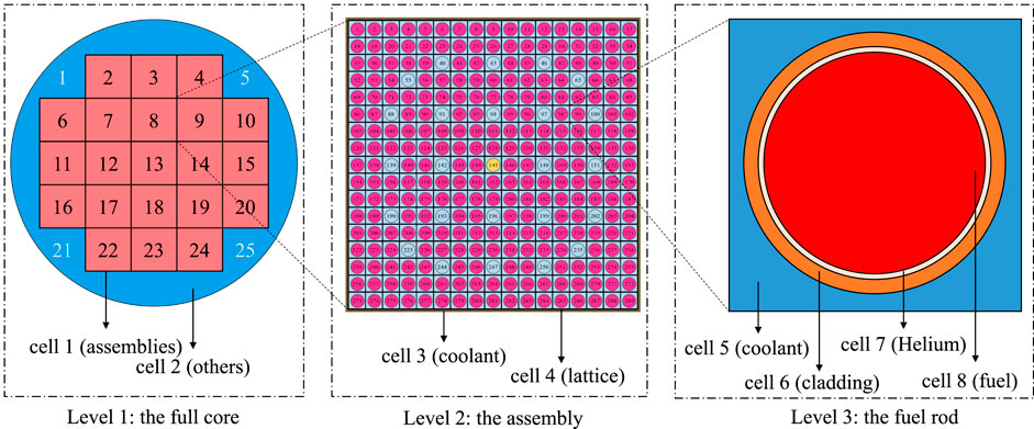
FIGURE 1. Hierarchical repeated geometry structure of the reactor core in the NEA Phase II-C Burn-up credit criticality benchmark.

In Figure 1, Level 1 demonstrates the simplified outline of the whole core, which consists of two cells, one for the assemblies (cell 1) and the other (cell 2) for the baffle, water reflector, core barrel, pressure vessel, etc. The 21 assemblies are built with a 5-by-5 repeated structure, and the four corners are excluded. Assembly 8 is expanded as Level 2 in the figure, which includes the coolant in between the assemblies (cell 3) and the repeated lattice (cell 4). The repeated lattice has 264 fuel rods, 24 control rods (or guide tubes), and 1 instrument tube (or guide tube). The fuel rod with index 98 is expanded as Level 3, which has 4 cells, the coolant (cell 5), the cladding (cell 6), the helium gap (cell 7) and the fuel pellet (cell 8).

For a typical fresh reactor core, the cells in Level 3 are usually modeled the same in all of the fuel rods, guide tubes, control rods, and instrument tubes specifically, as they have common geometrical structures and material compositions. Therefore, in the RSG representation, they can be modeled as one cell rather than thousands or even millions of cells, thus reducing the memory footprint. However, for problems with burnup, thermal-hydraulic feedbacks, etc., the material or the temperature of those cells can be different from others, which leads to the requirement to identify each cell. A straightforward idea is to trace all the cells along the hierarchical tree (Figure 2) levels, record all the cell indices from the root to the cell, and form a cell vector. For example, cell 8 in Figure 1 can be tracked from the root in Figure 2 as the green circles and represented as “1 > 8 > 4 > 98 > 8”. The “$>$” is the delimiter between different levels, indicating that the left values are from higher levels. The integers in the cell vectors are the cell indices or the repeated lattice indices. Note that the two “8”s in the cell vector have different meanings—the first one is the index of the assembly in the core lattice, and the second one is the cell index of the fuel pellet.

FIGURE 2

FIGURE 2. Tree view of the hierarchical repeated geometry structure of the reactor core in the NEA Phase II-C burn-up credit criticality benchmark.

2.2 Definition of the hash function of the cell vectors

With the cell vectors, we may identify each cell in the RSG and thus build a map between the cell vectors and the cell parameters such as the material composition and temperature. As shown in Figure 3, a straightforward method is to build a cell vector list and a parameter list. Then, when we need to obtain the parameter for a certain cell vector, we may sequentially walk through the first list to find the target cell vector and then use the index to obtain the parameter from the second list. However, the time complexity of the averaged sequential search is O(n), which may take an excessive amount of time on millions of cell vectors.

FIGURE 3

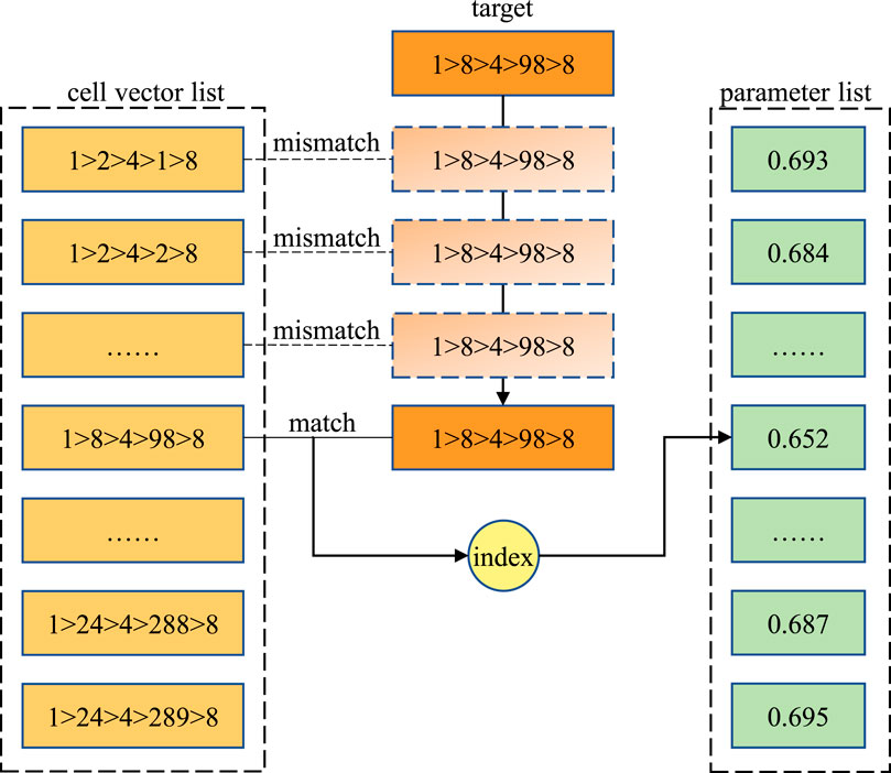
FIGURE 3. Sequential matching method for locating the target cell vector and fetching the corresponding coolant density. The values are only for demonstration.

Therefore, as shown in Figure 4, modern Monte Carlo particle transport codes may map the cell vectors to the indices directly with a function. The function is called the hash function, and the method is called the hash mapping method. The hash function on the cell vectors can be defined as follows:

$hash\left(\vec{c}\right)=f\left(\vec{c}\right)=f\left(c_1,c_2,\dots ,c_k\right)(1)$

where $\vec{c}$ is the cell vector, k is the length of the cell vector and c_i is the i-th cell or lattice index. The hash value $hash(\vec{c})$ is an integer that is used as the key to fetch the corresponding parameter from the key-value map. Actually, the key-value relationship (K-V mapping) in Figure 4 is also a hash function, which is internally implemented in many programming languages. The hash function is not dependent on the total number of cell vectors n, and the time complexity of the hash mapping method is typically O (1). However, hash functions cannot guarantee that the hash values for all the cell vectors are unique. When t different cell vectors yield the same hash values, the algorithm may drop to O(t) complexity to sequentially check each cell vector, and this phenomenon is called hash collisions. An effective hash function $f(\vec{c})$ should be simple but have fewer collisions. The simplicity promises that the calculation of the hash function does not take too much time, and the fewer collisions guarantee that the averaged time complexity is still O (1).

FIGURE 4

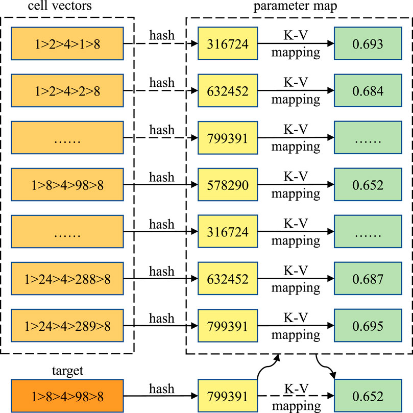
FIGURE 4. Hash mapping method for locating the target cell vector and fetching the corresponding coolant density. The values are only for demonstration.

Note that, in fact, the time complexity should be related to the length of the cell vector k, that is, O$(f(\vec{c}))$. However, as k is typically very small when compared with n, and the hash function ought to be very simple, the calculation time for the hash function should be bounded by a small value, and thus, the time complexity of hash functions can be represented as O (1).

2.3 Typical hash functions for cell vectors in reactor monte carlo simulations

There are innumerable hash functions to choose, and in this section, we introduce some typical ones that are commonly used in Reactor Monte Carlo simulations.

2.3.1 The base-p hash function

She et al. (2013) applied the base-p hash function in Monte Carlo simulations, which is a common hash function for vectors that has been mathematically proven effective. The base-p hash function can be illustrated as Eq. 2 below:

$hash\left(\vec{c}\right)=f_{\mathit{base-p}}\left(\vec{c}\right)=\sum _{i=1}^k{c}_i{p}^{i-1}(2)$

where p is a predefined constant integer. This hash function is very simple, and there are only (k + 1)k/2–1 operations. In practice, this function can be further optimized with Horner’s scheme (Jiushao Qin’s scheme in China) to a total of 2 (k − 1) operations in Eq. 3, which has been proven optimal by Cajori (1911):

$\begin{array}{ll}\hfill f_{\mathit{base-p}}\left(\vec{c}\right)& =\sum _{i=1}^k{c}_i{p}^{i-1}\hfill \\ \hfill & =c_1+p\left(c_2+p\left(c_3+\cdots +p\left(c_{k-1}+p{c}_k\right)\cdots \right)\right)\hfill \end{array}(3)$

In actual calculations on computers, a modular calculation should be added to Eq. 2 due to storage limits for integers:

$f_{\mathit{base-p}}\left(\vec{c}\right)=\sum _{i=1}^k{c}_i{p}^{i-1}\mathrm{mod}\mathcal{M}(4)$

where $\mathcal{M}$ is the module caused by the overflow from large p or k values, and $\mathcal{M}$ depends on the hash value type and the storage limits of the machine. Typically, $\mathcal{M}$ equals the maximum of the possible unsigned integer in the computer plus one, that is, $\mathcal{M}={\mathcal{L}}_{\mathit{max}}+1$, where ${\mathcal{L}}_{\mathit{max}}$ is the upper limit of the possible unsigned integer on the machine. For example, if we use the “unsigned long long” type to save and calculate the hash value on a 64-bit machine, ${\mathcal{L}}_{\mathit{max}}$ should be 2⁶⁴ − 1, and the module $\mathcal{M}$ equals 2⁶⁴.

If we change $\mathcal{M}$ in Eq. 4 from a machine-defined value to a manually predefined coefficient, we may obtain a more general hash function. In this function, $\mathcal{M}$ is usually defined as a large prime to flatten the probability distribution for all possible hash values, which is mathematically proven to be able to reduce the collision probabilities (Carter and Wegman, 1979). Practically, however, powers of 2 are widely used, such as 2⁶⁴ above, to reduce the calculation complexity on computers.

The core problem for this hash method is the selection of p and $\mathcal{M}$. Generally, $\mathcal{M}$ should be set larger to broaden the domain of the possible hash values, but in regard to choosing a proper value for p, things become somewhat tricky. Below are some considerations on the selection of p:

•Ideal Situation: When all the indices in the cell vectors are less than p, and the results of Eq. 2 are all no more than the maximum integer L_max on the machine, there will be no hash collisions. Therefore, a large value of p may be better.

•SmallerpIssue: When there are some indices larger than p, hash collisions may occur regardless of what modular $\mathcal{M}$ is. For example, cell vector “1 > (p + 1) > 3” may share the same hash value with “1 > 1 > 4”. It is common to have similar cell vectors like those two in reactor simulations, where the second level can be the RSG lattice of the assembly and the third level refers to the cells in the fuel pins. Additionally, such cases may also occur occasionally in non-RSG parts when the model is very complicated and has too many cell vectors. Smaller p Issue may become vital in complicated models, as there may be too many cells and thus the cell indices may be large.

•LargerpIssue (Overflow Issue): When p is defined too large, overflows will become increasingly common in Eq. 2. Consequently, cell vectors with large indices may have chance to collide with those with small indices. Moreover, in most scenarios, overflows should be avoided in hash function designs because the processing of overflows can be different on different hardware architectures, which may lead to unpredictable calculation results.

•p-$\mathcal{M}$Interactions: In Eq. 4 where $\mathcal{M}$ is manually defined, additional calculations have to be conducted to avoid overflows, that is, modular operations have to be performed not only once at the end but possibly once after only one or a few multiplication and addition operations. Specifically, when using Horner’s scheme in Eq. 4, modular operations should be performed no less than k − 1 times, that is, once for a bracket. Additionally, to guarantee that the multiplications by p close to the brackets in Eq. 3 will not cause overflows, $p\mathcal{M}\le {\mathcal{L}}_{\mathit{max}}$ should be satisfied.

In summary, p should not be too small or too large, and when $\mathcal{M}$ is manually set, it should be a large prime but fulfill $p\mathcal{M}\le {\mathcal{L}}_{\mathit{max}}$. Chances of hash collisions always exist when Eq. 5 below cannot be guaranteed true for all the cell vectors. Therefore, in practical use, the parameters must be optimized with testing.

$\underset{1\le i\le k}{\max }{c}_i\le p(5)$

2.3.2 The shift hash function

The shift hash function was proposed and implemented by Guo et al. (2021). The basic idea of the shift hash function is to fully utilize the memory space of the integer value type and substitute multiplication and addition operations with bit operations to accelerate the calculations.

Assuming that there are totally n cell vectors in the model, we can represent the i-th cell vector with Eq. 6 below:

${\vec{c}}_i=\left(c_{i1},c_{i2},\dots ,c_{i{k}_i}\right)(6)$

where k_i is the length of the i-th cell vector and c_ij is the j-th component of the cell vector. The shift hash method merges the binary representations of the indices and adds some zeros to align each level, as the following steps demonstrate and shown in Figure 5:

i. Find the maximums of each level.

$m_j=\underset{1\le i\le n}{\max }{c}_{ij}(7)$

FIGURE 5

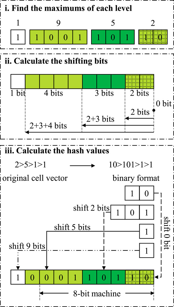
FIGURE 5. Working process of the shift hash mapping method.

If some of the cell vectors are shorter than others, the corresponding indices c_ij in Eq. 7 can be substituted by zeros.

ii. Calculate the shifting bits

Calculate the binary bit numbers of the maximums in Step 1 by logarithmic operations. Those values are the fewest bits to contain all the indices at certain levels.

$b_j=\mathrm{fl}\mathrm{o}\mathrm{o}\mathrm{r}\left(\ln m_j\right)+1(8)$

where b_j is the bit number of the j-th level’s maximum m_j and “floor” is a function to round down float values. For instance, when m_j is 203, its binary representation would be 0b11001011 with 8 bits, so b_j equals 8. Then, the bit numbers are accumulated to obtain the actual shifting bits.

$s_1=0,s_j=\sum _{t=1}^{j-1}{b}_t(9)$

where s_j is the bit number at the right side of the j-th level.

iii. Calculate the hash values

$hash\left(\vec{c}\right)=f_{\mathit{shift}}\left(\vec{c}\right)=\sum _{j=1}^k{c}_j{2}^{s_j}(10)$

In practical calculations, we can use bit left shift by s_j bits to perform the multiplications by $2^{s_j}$ and then use bit-or operation to sum all the terms. When the final result exceeds the upper limit of the machine ${\mathcal{L}}_{\mathit{max}}$, the hash function should be:

$f_{\mathit{shift}}\left(\vec{c}\right)=\sum _{j=1}^k{c}_j{2}^{s_j}\mathrm{mod}\left({\mathcal{L}}_{\mathit{max}}+1\right)(11)$

Comparing Eqs 4, 11, we may find that the two equations are similar. The shifting hash method can be regarded as a special form of the base-p hash method, where p equals 2 and some indices in Eq. 4 are 0.

As the b_i values are carefully assigned to confirm that $2^{b_i}$ is larger than all the indices on Level i, the shift hash method succeeds in avoiding the hash collisions caused by the Smaller p Issue mentioned in Section 2.3.1, and realizes bijection between the cell vectors and the hash values. Practical uses of the two hash methods have proven that the shift hash method has fewer collisions, and more experiments can be found in Section 4.2.

However, the shift hash method cannot solve the Overflow Issue in Section 2.3.1. Even worse, collisions will become very common when overflows occur, because the module ${\mathcal{L}}_{\mathit{max}}+1$ is also a power of 2, and consequently, the overflowed left shifting bits are simply erased.

For example, assuming that we are using an 8-bit machine where an integer occupies 8 bits and we have a total of 45 cell vectors 2 > (1 : 5) > (1 : 9) > 1, where the second and third levels are RSG lattices that represents the core lattice and the assembly lattice. “1:5” means the possible values are from 1 to 5. Then, we may follow the steps to calculate m_j and b_j as below:

$\begin{array}{c}\left\{m_4,m_3,m_2,m_1\right\}=\left\{\mathrm{1,9,5,2}\right\}\\ \left\{b_4,b_3,b_2,b_1\right\}=\left\{\mathrm{1,4,3,2}\right\}\end{array}(12)$

therefore, the hash values of the cell vectors “2 > 5 > 1 > 1” and “2 > 5 > 9 > 1” can be calculated with the steps above as 0b1000110110 and 0b1100110110. The detailed calculation process for “2 > 5 > 1 > 1” is represented in Figure 5. Because it is an 8-bit machine where ${\mathcal{L}}_{\mathit{max}}$ should be 0b11111111, the final hash values of the 2 cell vectors from Eq. 11 are both 0b110110, that is, 54. Moreover, this collision is not related to the first, second and fourth indices, which means that “a > b > 1 > c” will always collide with “a > b > 9 > c”, that is, cells in fuel rods with index 1 and 9 of different assemblies may always share the same hash values, indicating an enormous number of collisions. To handle that issue, overflows have to be avoided, and thus larger problems may require longer storage types to contain the hash values. Specifically, if the 32-bit shift hash method with the “unsigned int” type may overflow for large reactor simulations, we may change the integer type to 64-bit “unsigned long long” or even 128-bit “__int128”.

3 CRC hash method

Cyclic redundancy check (CRC) is commonly used in error-detecting scenarios to discover accidental changes to digital data during network or storage transmission (Peterson and Brown, 1961). The CRC algorithm accepts blocks of data and calculates a short check value based on the remainder of a polynomial division. The check value will then be transmitted together with the original data and compared with the result from the recalculation on the received data for error detection.

3.1 The applicability of the CRC algorithm in reactor Monte Carlo simulations

As the check value from CRC has a fixed length, the CRC algorithm can be used as a hash function. Furthermore, the cell vectors in reactors have a special feature in that there may be many vectors with only one or two different indices such as “2 > (1 : 5) > (1 : 9) > 1” above, mainly from the RSG lattices. If we regard those slight differences as errors in signal transmission, then CRC is quite suitable to detect and distinguish different cell vectors.

It has been mathematically proven that n-bit CRC can detect any single error burst no longer than n bits, and longer error bursts can be detected with (12⁻ⁿ) probability (Koopman, 2002). When n equals 32, the undetected fraction 2⁻ⁿ is approximately 2.3 × 10⁻¹⁰, and when n is 64, it is only around 5.4 × 10⁻²⁰, which indicates that the collision probability of the CRC hash mapping method is extremely low. In the high-fidelity Monte Carlo simulations for large commercial reactors, there can be up to 10⁸ cells in total; thus, the probability of no collisions with the 64-bit CRC hash mapping method should be:

$\begin{array}{ll}\hfill \mathrm{P}\left(\text{no\hspace{0.17em}collisions}\right)& \approx {\left(1-p\right)}^{\frac{N\left(N-1\right)}{2}}=1-\frac{N\left(N-1\right)}{2}p+O\left(N^4{p}^2\right)\hfill \\ \hfill & \approx 99.973\%+O\left(10^{-8}\right)\hfill \end{array}(13)$

where N is the number of cell vectors (10⁸) and p is the collision probability of any two cell vectors (5.4 × 10⁻²⁰). Note that there may be some bias in the distribution of the cell vectors and there is an assumption in Eq. 13 that collision incidents are independent, so the actual probability of no collisions may differ from the value of 99.973%. However, this analysis may guarantee that the 64-bit CRC hash mapping method is sufficient to minimize the collision probability and thus works well for high-fidelity reactor simulations.

3.2 Calculations in the CRC algorithm

The commonly used CRC algorithm can be formed as a polynomial division on the Galois field GF (2). The two elements in GF (2) are typically 0 and 1, and the addition operator on GF (2) is XOR (exclusive disjunction). In the polynomial division, the original data forms the input polynomial, a predefined polynomial serves as the divisor, and the remainder polynomial gives the final check value. An n-bit CRC algorithm has an n-order polynomial as the divisor. The selection of the polynomial is the core problem in CRC algorithm implementation, as a proper divisor may minimize the overall collision probabilities.

Take a 3-bit CRC with a divisor polynomial x³ + x + 1 as an example. The cell vector “1 > 1 > 5 > 2” on a 4-bit machine can be converted into a sequence of binary data “0010,0101,0001,0001”, where the order is reversed to put indices on bottom levels prior to the upper ones. Then, the merged binary value should be padded with n zeros; thus, we obtain “0010010100010001000”, which can be represented as 2¹⁶ + 2¹³ + 2¹¹ + 2⁷ + 2³. If we substitute 2 with x, we may obtain the input polynomial x¹⁶ + x¹³ + x¹¹ + x⁷ + x³. Afterward, we may have

$\begin{array}{ll}\hfill x^{16}+x^{13}+x^{11}+x^7+x^3& =\left(x^3+x+1\right)\left(x^{13}+x^{11}+x^9+x^7\right.\hfill \\ \hfill & \left.+x^6+x^5+x^4+x+1\right)\oplus \left(x^2+1\right)\hfill \end{array}(14)$

that is,

$x^2+1=\left(x^{16}+x^{13}+x^{11}+x^7+x^3\right)\mathrm{mod}\left(x^3+x+1\right)(15)$

where the addition operator on GF (2) is actually the XOR operator ⊕. The remainder polynomial x² + 1 indicates that the final 3-bit CRC check value is 0b101.

Because the quotient polynomial has no use in the process, the algorithm can be simplified to only calculate the remainder, as shown in Figure 6. We may first align the divisor to the left most “1” and perform the XOR operation on the input binary sequence. Then, the divisor is moved to the left most “1” of the result and XOR operations are recursively performed until the divisor arrives at the end. The remaining values represent the remainder of the polynomial division, that is, the CRC check value.

FIGURE 6

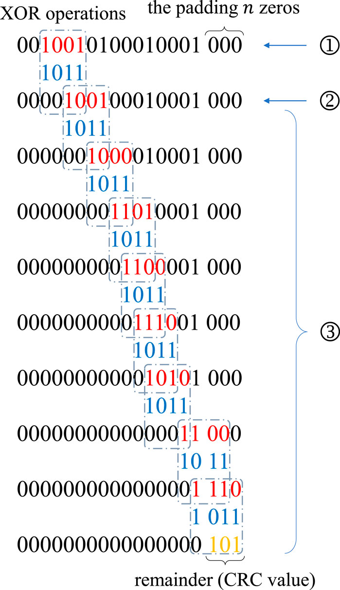
FIGURE 6. The simplified calculation process of a 3-bit CRC algorithm on the example data flow “0,010, 0,101, 0,001, 0,001” from the cell vector “1 > 1 > 5 > 2”. ①: Calculation starts from the first non-zero bit; ②: Remainder is from the XOR operation between the input and the divisor; ③: Move the divisor to the next non-zero bit and recursively apply XOR operations.

3.3 Acceleration of the CRC algorithm

3.3.1 Precalculated CRCTable

In practical implementations of the CRC algorithm, there will be a precalculated table to store the results from calculations on several bits. For example, the 32-bit CRC algorithm implemented and introduced by Corporation (2019) has a CRCTable of 256 8-bit constants, where each value is the CRC calculation on the possible 8-bit integers from 0 to 255. In this way, the movement of the divisor in ③ of Figure 6 can be increased to 8 bits—the looked-up table value is simply fetched as the result of the repeated XOR operations on the 8 bits and then concatenated with the remaining bits.

3.3.2 Batch processing

In addition to the precalculated CRCTable, several 8-bit blocks can be batched together for processing, and then the results are merged to obtain the final value. This strategy may optimize the use of the cache and registries in the machines and thus accelerate the calculation.

3.3.3 Other accelerations

As the CRC algorithm is significant in many modern applications with data check requirements, chip manufacturers have implemented it in hardware. For example, CRC32 has been implemented in SSE 4.2 as “crc32” instruction for Intel CPUs (Gopal et al., 2011).

For earlier CPUs that do not support SSE 4.2, there are also some open-source asm codes that are faster than C/C++ implementations, such as the ISA-L library¹ by Intel Corporation (Intel Cooperation, 2023). ISA-L library has also provided some acceleration solutions for the 64-bit CRC algorithm and many other CRC variants.

3.4 Implementation in RMC code

The Reactor Monte Carlo code RMC is a particle transport code developed by the Reactor Engineering Analysis Lab (REAL) at Tsinghua University, Beijing, China, as a software kit for reactor analyses on high-performance computing systems (Wang et al., 2015). Many features have been developed in RMC to meet the requirements of reactor simulations, including criticality, shielding, burnup, transient, and multi-physics simulations. The high-fidelity simulation capability of RMC has been validated in the multi-physics simulation of the BEAVRS two-cycle benchmark (Horelik et al., 2013) in Wang et al. (2017) and the VERA core physics benchmarks (Godfrey, 2014) in Luo et al. (2017), Luo et al. (2020) and Ma et al. (2019), and transient simulations of the C5G7-TD benchmarks (Hou et al., 2017) in Guo et al. (2020).

Different hash mapping methods have been introduced in RMC, including the base-p hash method (She et al., 2013) and the shift hash mapping method (Guo et al., 2021). However, with the increasing need for higher fidelity simulations of large commercial reactors, the shortcomings of the two hash methods have become crucial because probabilities of hash collisions are rising. Therefore, we have implemented the CRC64 hash mapping method in RMC and accelerated it with ISA-L’s asm implementations (Intel Cooperation, 2023).

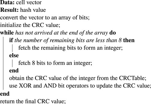
The pseudo code of the CRC hash mapping method implemented in RMC is presented in Algorithm 1 below. The precalculated CRCTable is applied to process 8 bits in each loop to accelerate the calculations. In practice, the initialization and the while loop in Algorithm 1 can be substituted by the calling of the “crc64_ecma_refl” function in the ISA-L library. The “crc64_ecma_refl” function is implemented and optimized using assembly language by Intel Cooperation, and thus may be used to further accelerate the calculations of the CRC hash values.

Algorithm 1. The pseudo codes for CRC64 hash mapping method implemented in RMC code.

From the analysis in Section 3.1, the probability of possible collisions for a large reactor simulation problem with 10⁸ cell vectors is as small as 0.027%, which is sufficient for reactor simulations currently and in the near future. For the far future, a 128-bit CRC hash mapping method can be easily implemented to support up to 10¹⁶ cell vectors.

4 Validations for the CRC hash method

In this section, we will examine the CRC hash method and compare it with other hash methods both in virtual applications for collision and speed tests, and in practical simulations for integrated tests.

4.1 Collision test in virtual applications

To test the collision probabilities of different hash methods, we generate a large number of cell vectors and calculate their hash values with different hash functions. The collision number is defined as the total number of cell vectors minus the number of unique hash values.

We designed two random cell vector generators: a uniform generator and a bias-imitating random generator. The former generator is simply generating indices at each level from a uniform distribution, and the latter may try to imitate the distribution of the cell vectors in practical commercial reactors.

4.1.1 Experiment with the uniform generator

To generate a cell vector, we may first define the length of the vector and then sequentially generate each index. Therefore, we define 4 coefficients in the uniform cell vector generator:

•L_l the lower bound of the vector lengths

•L_u the upper bound of the vector lengths

•I_l the lower bound of the cell or lattice indices

•I_u the upper bound of the cell or lattice indices

For each cell vector, we may first generate the vector length L uniformly from [L_l, L_u] and then repeatedly generate the cell or lattice index uniformly from [I_l, I_u] for L times. Additionally, there are two non-generator parameters:

•N the number of cell vectors to be generated

•R the number of repetitions on hash calculations

R is defined to imitate the actual scenario where the hash function may be called several times on the same cell vector at different times. In this way, the estimations of calculation speeds may become more realistic and reliable.

Typically, there are no more than 10 levels and 10⁸ cell vectors in a reactor core simulation problem. Therefore, we set the four bounds as [L_l, L_u] = [8, 12] and [I_l, I_u] = [1, 99999999], and the total number as N = 10⁸ and N = 10⁹ in two experiments for the current and even more complicated models. To keep the total calculation tasks NR the same in the two experiments, we set R as 100 and 10 specifically.

There are six hash methods or their variants engaged in the experiments: the base-p hash method where p is 499 or 49,999 (both are primes), the shift hash method using a 64-bit integer type or 128-bit integer type, the original CRC64 hash, and the CRC64 method accelerated by ISA-L. The results of the experiments are demonstrated in Table 1(N = 10⁸); Table 2(N = 10⁹). To reduce the noise from random generation, all the experiments are performed 5 times, and then the averages and their standard deviations are listed in the two tables.

TABLE 1

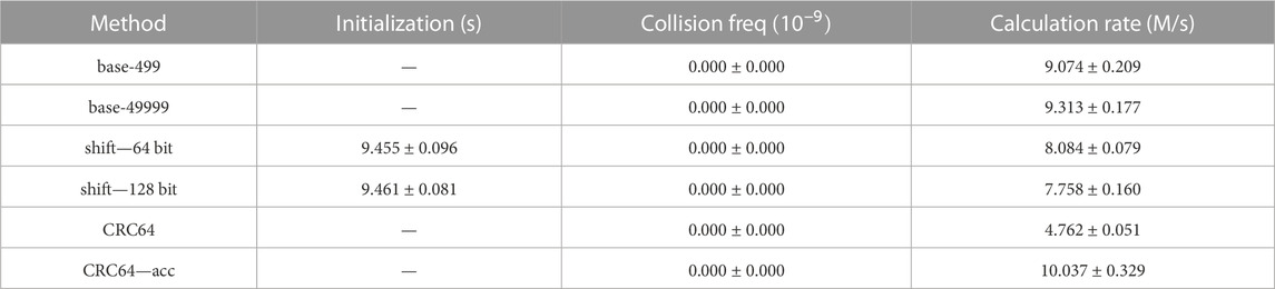
TABLE 1. Collision and speed test for different hash methods on 10⁸ uniformly sampled cell vectors with 100 repetitions. The experiments are performed 5 times to obtain the average values and their deviations.

TABLE 2

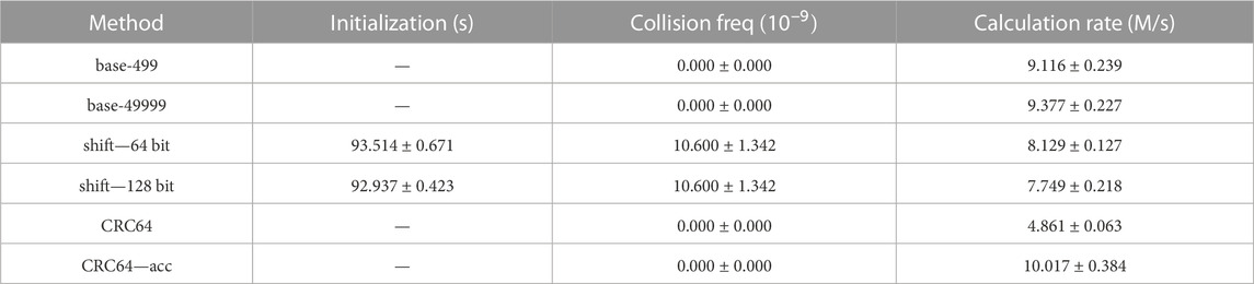
TABLE 2. Collision and speed test for different hash methods on 10⁹ uniformly sampled cell vectors with 10 repetitions. The experiments are performed 5 times to obtain the average values and their deviations.

In each experiment, we may first generate the cell vectors randomly, during which time a unique test is performed to guarantee that there are no duplicates in the N cell vectors. Then, the participating hash methods are examined sequentially. The hash methods are all split into three stages: initialization, collision test, and repetition speed test:

1. Initialization: Shift hash methods need to calculate the maximums and moving bits for each level during their initialization, and thus, we record the time cost for the initialization stage in our experiments. Hash methods with no initialization are marked as “-” in the corresponding column of the two tables.

2. Collision Test: As it is meaningless to repeat in collision tests, we iterate over the whole set of cell vectors only once to find the hash collisions. The collision frequencies in the two tables are the collision numbers divided by the numbers of hash function calls.

3. Repetition Speed Test: To obtain a better estimated calculation speed, the cell vectors are fed into the hash function for R times. Note that the R repetitions are calculated on the same set of cell vectors, while the 5 runs mentioned in the tables are carried out on different sets of randomly generated cell vectors. Additionally, the unit “M/s” in the two tables refers to million cell vectors processed per second.

From the comparisons in Tables 1, 2, we may notice the following:

1. Initialization: The shift hash methods are the only ones that require initializations among the involved hash methods. The time cost for initialization is around 92 s for 10⁹ cell vectors, that is, 10.81 M/s, which is approximately the cost of 1 repetition. That is affordable for such a large model with so many cells.

2. Collision Test: The shift hash methods are the only ones where hash collisions occur. This phenomenon agrees with the analysis in Section 2.3.2 that the overflow issue in the shift hash methods may lead to more collisions. As the distribution of actual cell vectors may differ from the uniform distribution in this section, the collision probabilities of those hash methods in practical Monte Carlo simulations may vary from the values in Tables 1, 2.

3. Speed Test: Shift hash methods are slightly slower than base-p hash methods, which may result from more operations in shift hash methods and automatic optimization of CPU multiplication operations in base-p hash methods. The CRC64 hash method is the slowest, which is reasonable, as the calculation process is the most complicated. However, as CRC is a common algorithm to be applied in many applications, research on the acceleration of CRC is continuously pushed forward. In our experiment, the CRC hash mapping method accelerated by ISA-L is the fastest hash method among the 6 methods involved.

4. Others: The speed test results from experiments on 10⁸ and 10⁹ cell vectors are similar, which indicates that the values and patterns can be applied to other scales.

Generally, in this uniform generator scenario, the accelerated CRC64 hash method outperforms the others in all aspects.

4.1.2 Experiment with the bias-imitating random generator

As the distribution of cell vectors in reactors may be biased from uniform sampling, the collision probabilities in Section 4.1.1 may differ from the actual performance in reactor simulations. Therefore, in this section, we create a set of cell vectors that imitates the actual distribution to correct this bias.

As shown in Figure 2, the actual CSG geometry is defined as a tree, where tree nodes are universes or cells filled with universes, leaf nodes are simple cells, and cell vectors are the paths from the root to the leaves. Each level of the tree may refer to the core, the assemblies or the pins. Typically, the indices for each level tend to be set as continuous integers, and indices between different levels may differ greatly. Accordingly, we designed simple Python scripts to imitate and generate the geometry tree and then traverse the tree to obtain the cell vectors. The Python scripts and the README. md file are attached in the Supplemental Materials. Readers may reproduce the datasets of cell vectors used in our experiments.

The overall experimental settings are similar to those in Section 4.1.1, except that the generator is substituted by the bias-imitating generator. The experimental results are presented in Tables 3, 4, 5. As the cell vectors are pre-generated and then kept fixed during each experiment, there are no random errors; thus no repetitions are performed and consequently there are no deviation values in the tables. Additionally, we add a base-500 hash mapping method in the comparison to check whether prime numbers work better.

TABLE 3

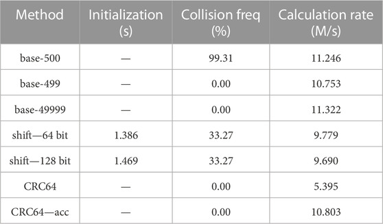
TABLE 3. Collision and speed test for different hash methods on bias-imitating samples, 10 repetitions. Parameters: 26.028 million cell vectors, 1,000 as the interval, single filling.

TABLE 4

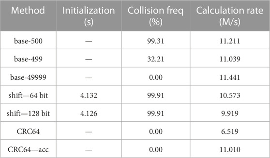
TABLE 4. Collision and speed test for different hash methods on bias-imitating samples, 10 repetitions. Parameters: 78.030 million cell vectors, 1,000 as the interval, multiple filling.

TABLE 5

TABLE 5. Collision and speed test for different hash methods on bias-imitating samples, 10 repetitions. Parameters: 78.030 million cell vectors, 10,000 as the interval, multiple filling.

The three experiments are distinct from each other in the “interval” value and single/multiple filling. The “interval” value is used to generate the cell indices in the model, which is specifically the interval of the cell indices between neighboring universes. For example, if the interval is 1,000 and the first cell of the first Universe has an index of 1,001, then the index of the first cell of the second Universe should be 2001. Single or multiple filling is used to define whether there may be only a single cell or multiple cells that are filled with the same RSG lattice. Multiple filling models are widely used in burnup simulations. Readers may obtain more insights into those hyperparameters from the reproduced datasets.

From the tables, we may find that, among the three experiments, the CRC hash methods are the only ones that have no hash collisions. Other hash methods may have no collisions for some cases but show high collision probabilities for others, which may cause severe problems in certain practical applications.

The base-500 hash mapping method results in high collision probabilities in all the three cases, mainly because the interval 1,000 and 10,000 can be exactly divided by the base 500, causing carriages in the hash function calculations like the example “1 > (p + 1) > 3” and “1 > 1 > 4” in Section 2.3.1.

The base-499 and base-49999 hash mapping method have no collision in the first case because this case is the simplest. However, when handling the last two complicated cases, collisions may occur because the cell indexes can be larger than the base values. As 499 and 49,999 are primes, the collisions caused by carriages may occur for one method but not occur for the other, which leads to the large differences of collision probabilities.

The shift hash mapping method using 64-bit integers or 128-bit integers results in around 33% hash collision probabilities in the first case and more than 99% in the last two cases. That is because the last two cases have larger cell indexes, which may cause more overflows in the shift hash mapping method and thus higher hash collision probabilities.

Collisions may become a critical problem for shift hash methods as they collide in all the three experiments. For base-p hash methods, prime values 499 and 49,999 work better than 500 in collision probabilities and have similar calculation speeds, but they still cannot handle all the cases, which agrees with the theoretical analyses in Section 2.3.1.

Conclusions drawn from the initialization and calculation speed columns are similar to those in Section 4.1.1: the initialization costs from shift hash methods are acceptable and the accelerated CRC hash method is comparably fast as the base-p hash methods and shift hash methods. The accelerated CRC hash method did not outperform the base-p hash methods in calculating speed, mainly because the cell vectors are set to be no longer than 7, which is shorter than those in Section 4.1, and thus the acceleration effect is minor.

Overall, the experiments in this section reveal that bias of the cell vectors in practical applications may lead to a severe hash collision problem, especially in complicated full core burnup problems. The accelerated CRC hash method outperforms others with its comparable calculation speed and lowest probabilities of hash collisions, which may make it a better choice for Reactor Monte Carlo simulations.

4.2 Practical validation for the hash methods

Practical validation and comparison for the CRC hash method is performed on the VERA Problem #5 (Godfrey, 2014), a full core problem. The axial and radial profiles of the reactor core are shown in Figure 7. As RSG cell identification will not be triggered in criticality simulations, we add a burnup step to the core to examine the performance of the hash methods. 500,000 particles are simulated in each cycle, and 200 cycles are calculated in a burnup step. The calculations are all carried out on a machine with the AMD Ryzen 3,990X processor and 252 GB memory. Note that as hash collisions are difficult to handle in practical implementations for Reactor Monte Carlo simulations, we carefully modeled the reactor core to guarantee that there were no collisions in any involved hash mapping method.

FIGURE 7

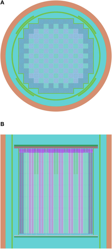
FIGURE 7. Radial and axial profiles of the VERA Problem #5 reactor core (Godfrey, 2014), drawn by the RMC code. (A): radial profile; (B): axial profile.

As shown in Table 6, the eigenvalue k_eff values calculated from different hash methods agree with each other very well - all of them are within twice the standard deviation. Due to the use of OpenMP, some differences may exist in the particle histories and the total number of hash function calls, thus causing the eigenvalues to be different. As the total hash function calls are also different, we may focus on the calculation speed rather than the total time.

TABLE 6

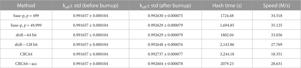
TABLE 6. Burnup simulation results for the VERA Problem #5 core.

In the actual simulation processes, a single call of the hash method may take less than 1 microsecond, and the hash function calls are not continuously performed. Therefore, it is difficult to precisely record the time consumption of all the hash function calls, and the uncertainties of the time-related values may be large and difficult to be quantified. Consequently, only large differences in Table 6 may reveal some conclusions.

As indicated from the calculation speeds shown in Table 6, the accelerated CRC method has greatly improved the original CRC, and outperforms the 128-bit shift hash method. The two base-p methods and the 64-bit shift hash method performs a little better in this case. However, this model is carefully modeled to avoid any collisions, and when applied on more complicated models, those three methods may crash, as analyzed in Section 4.1. Moreover, the calculation speeds here are much faster than those in Section 4.1. That is because the cell vectors here are no longer than 5, which are shorter than those in the virtual experiments. The shorter cell vectors may also limit the acceleration capability of the optimized CRC64 hash mapping method.

Combined with the results from Section 4.1, accelerated 64-bit CRC hash mapping method outperforms all the other methods in collision probabilities, and achieves a comparable calculation speed. Therefore, it should be a better choice for complicated high-fidelity reactor simulations.

5 Conclusion

The cyclic redundancy check (CRC) algorithm is analyzed and used to construct a new hash method in reactor simulations. This hash mapping method achieves an O (1) time complexity to handle the cell identification problem in RSG models. We first analyze the characteristics of the cell vectors in the RSG models and find that the burst error detection capability of the CRC algorithm makes it an ideal hash mapping method for reactor simulations. Then, we implemented and optimized the CRC hash mapping method in the RMC code and compared it with other hash methods in both virtual and practical scenarios. The experiments show that the CRC hash mapping method has a comparable calculation speed and much lower collision probability, which demonstrates that the CRC hash method is a more suitable hash method to be applied in RSG models, especially for complicated problems. The collision probabilities in the experiments can be reduced from more than 99% with other hash methods to 0% with the proposed CRC hash method, while the calculating speed is still comparable.

In this work, the CRC hash mapping method was implemented in all the features of RMC that are related to cell identification and distributed parameter indexing. As CRC is a common and well-known algorithm researched around the world, further improvements in CRC will continuously benefit our applications in Reactor Monte Carlo simulations.

Data availability statement

The original contributions presented in the study are included in the article/Supplementary Material, further inquiries can be directed to the corresponding author.

Author contributions

KL: conceptualization, methodology, investigation, software, validation, formal analysis, writing-original draft NA: resources, methodology, software HL: conceptualization, validations SH: writing-review and editing, supervision KW: project administration, funding acquisition, supervision. All authors contributed to the article and approved the submitted version.

Funding

This work was supported by the National Natural Science Foundation of China (Grant Nos 11775126 and 11775127).

Conflict of interest

The authors declare that the research was conducted in the absence of any commercial or financial relationships that could be construed as a potential conflict of interest.

Publisher’s note

All claims expressed in this article are solely those of the authors and do not necessarily represent those of their affiliated organizations, or those of the publisher, the editors and the reviewers. Any product that may be evaluated in this article, or claim that may be made by its manufacturer, is not guaranteed or endorsed by the publisher.

Supplementary material

The Supplementary Material for this article can be found online at: https://www.frontiersin.org/articles/10.3389/fenrg.2023.1161861/full#supplementary-material

Footnotes

¹GitHub link: https://github.com/intel/isa-l

References

Briesmeister, J. F. (1993) LA-12625. New Mexico, United States: Los Alamos National Laboratory.Mcnp-a general Monte Carlo n-particle transport code.

Google Scholar

Cajori, F. (1911). Horner’s method of approximation anticipated by ruffini. Bull. Am. Math. Soc.17, 409–414.

CrossRef Full Text | Google Scholar

Carter, L., and Wegman, M. N. (1979). Universal classes of hash functions. J. Comput. Syst. Sci.18, 143–154.

CrossRef Full Text | Google Scholar

Corporation, M. (2019). 32-Bit CRC algorithm. Redmond, Washington, United States: Microsoft Corporation.

Google Scholar

Deng, L., Ye, T., Li, G., Zhang, B., and Shangguan, D. “3-d Monte Carlo neutron-photon transport code jmct and its algorithms,” in Proceedings of the international conference on physics of reactors (PHYSOR2014), Kyoto, Japan, September 2015.

Google Scholar

Fensin, M. L., James, M. R., Hendricks, J. S., and Goorley, J. T. “The new mcnp6 depletion capability,” in Proceedings of the International Congress on the Advances in Nuclear Power Plants, Chicago, Illinois, United States, June 2012, 24–28.

Google Scholar

Godfrey, A. T. (2014). VERA core physics benchmark progression problem specifications, Revision 4. Oak, North Carolina, United States: Physics Integration Oak Ridge National Laboratory.

Google Scholar

Gopal, V., Guilford, J., Ozturk, E., Wolrich, G., Feghali, W., Dixon, M., et al. (2011). Fast CRC computation for iSCSI polynomial using CRC32 instruction. Santa Clara, California, United States: Intel Corporation.

Google Scholar

Guo, X., Shang, X., Song, J., Shi, G., Huang, S., and Wang, K. (2020). Kinetic methods in Monte Carlo code rmc and its implementation to c5g7-td benchmark. Ann. Nucl. Energy151, 107864. doi:10.1016/j.anucene.2020.107864

CrossRef Full Text | Google Scholar

Guo, X., Shen, P., Li, K., Huang, S., Liang, J., and Wang, K. (2021). A hash mapping method using cell vectors in Monte Carlo code rmc. Ann. Nucl. Energy160, 108395. doi:10.1016/j.anucene.2021.108395

CrossRef Full Text | Google Scholar

Horelik, N., Herman, B., Forget, B., and Smith, K. (2013). Benchmark for evaluation and validation of reactor simulations (BEAVRS), v1.0.1. Massachusetts, MA, USA: MIT Computational Reactor Physics Group.

Google Scholar

Hou, J. J., Ivanov, K. N., Boyarinov, V. F., and Fomichenko, P. A. (2017). Oecd/nea benchmark for time-dependent neutron transport calculations without spatial homogenization. Nucl. Eng. Des.317, 177–189.

Google Scholar

Intel Cooperation, (2023). Intel® intelligent storage acceleration library. Santa Clara, California, United States: Intel Corporation.

Google Scholar

Koopman, P. “32-bit cyclic redundancy codes for internet applications,” in Proceedings International Conference on Dependable Systems and Networks (IEEE), Washington, DC, USA, June 2002, 459–468. doi:10.1109/DSN.2002.1028931

CrossRef Full Text | Google Scholar

Lax, D. M. (2015) Ph.D. thesis. Massachusetts, MA, USA: Massachusetts Institute of Technology.Memory efficient indexing algorithm for physical properties in OpenMC.

Google Scholar

Leppänen, J. (2013). Serpent–a continuous-energy Monte Carlo reactor physics burnup calculation code. Espoo, Finland: VTT Technical Research Centre of Finland.

Google Scholar

Luo, Z., Guo, J., Yu, G., Wang, K., and Liu, S. (2017). Solutions to vera core physics benckmark progression problems 1 to 6 based on rmc. Trans. Am. Nucl. Soc.143, 1235–1238.

Google Scholar

Luo, Z., Li, H., Yu, G., Ma, Y., Li, K., Guo, X., et al. (2020). Rmc/ctf multiphysics solutions to vera core physics benchmark problem. Ann. Nucl. Energy143. doi:10.1016/j.anucene.2020.107466

CrossRef Full Text | Google Scholar

Ma, Y., Liu, S., Luo, Z., Huang, S., Li, K., Wang, K., et al. (2019). Rmc/ctf multiphysics solutions to vera core physics benchmark problem 9. Ann. Nucl. Energy133, 837–852. doi:10.1016/J.ANUCENE.2019.07.033

CrossRef Full Text | Google Scholar

Neuber, J. C. (2008). Burn-up Credit criticality benchmark: Phase II-C: Impact of the asymmetry of PWR axial burn-up profiles on the end effect. Paris, France: Nuclear Energy Agency.

Google Scholar

Peterson, W. W., and Brown, D. T. (1961). Cyclic codes for error detection. Proc. IRE49, 228–235.

CrossRef Full Text | Google Scholar

Pratt, M. J. (2001). Introduction to iso 10303—The step standard for product data exchange. J. Comput. Inf. Sci. Eng.1, 102–103.

CrossRef Full Text | Google Scholar

Rearden, B. T., Petrie, L., Peplow, D. E., Bekar, K. B., Wiarda, D., Celik, C., et al. “Monte Carlo capabilities of the scale code system,” in Proceedings of the SNA+ MC 2013-Joint International Conference on Supercomputing in Nuclear Applications+ Monte Carlo (EDP Sciences), Paris, France, October 2014.

Google Scholar

Romano, P. K., and Forget, B. (2013). The openmc Monte Carlo particle transport code. Ann. Nucl. Energy51, 274–281.

CrossRef Full Text | Google Scholar

She, D., Liu, Y., Wang, K., Yu, G., Forget, B., Romano, P. K., et al. (2013). Development of burnup methods and capabilities in Monte Carlo code rmc. Ann. Nucl. Energy51, 289–294.

CrossRef Full Text | Google Scholar

Shen, P., Liang, J., Liu, S., and Wang, K. “Implementation and verification of the dagmc module in Monte Carlo code rmc,” in Proceedings of the 30th International Conference on Nuclear Engineering (ICONE 30), Virtual, Online, August 2022.

Google Scholar

Shriwise, P. C. (2018) Ph.D. thesis. Madison, WI, United States: The University of Wisconsin-Madison.Geometry query optimizations in CAD-based tessellations for Monte Carlo radiation transport.

Google Scholar

Shriwise, P., Zhang, X., and Davis, A. (2020). Dag-openmc: Cad-based geometry in openmc. Proc. Amer. Nucl. Soc. Winter Meet.122, 395–398.

CrossRef Full Text | Google Scholar

Sutton, T., Donovan, T., Trumbull, T., Dobreff, P., Caro, E., Griesheimer, D., et al. “The mc21 Monte Carlo transport code,” in Proceedings of the Joint international topical meeting on mathematics and computation and supercomputing in nuclear applications (M&C + SNA 2007), Monterey, California, United States, April 2007.

Google Scholar

Vazquez, M., Tsige-Tamirat, H., Ammirabile, L., and Martin-Fuertes, F. (2012). Coupled neutronics thermal-hydraulics analysis using Monte Carlo and sub-channel codes. Nucl. Eng. Des.250, 403–411.

CrossRef Full Text | Google Scholar

Wang, K., Li, Z., She, D., Liang, J., Xu, Q., Qiu, Y., et al. (2015). Rmc – A Monte Carlo code for reactor core analysis. Ann. Nucl. Energy82, 121–129. doi:10.1016/J.ANUCENE.2014.08.048

CrossRef Full Text | Google Scholar

Wang, K., Liu, S., Li, Z., Wang, G., Liang, J., Yang, F., et al. (2017). Analysis of beavrs two-cycle benchmark using rmc based on full core detailed model. Prog. Nucl. Energy98, 301–312.

CrossRef Full Text | Google Scholar

Wilson, P. P., Tautges, T. J., Kraftcheck, J. A., Smith, B. M., and Henderson, D. L. (2010). Acceleration techniques for the direct use of cad-based geometry in fusion neutronics analysis. Fusion Eng. Des.85, 1759–1765. doi:10.1016/j.fusengdes.2010.05.030

CrossRef Full Text | Google Scholar

Wu, Y., Song, J., Zheng, H., Sun, G., Hao, L., Long, P., et al. (2015). Cad-based Monte Carlo program for integrated simulation of nuclear system supermc. Ann. Nucl. Energy82, 161–168.

CrossRef Full Text | Google Scholar

Yu, J., Lee, H., Lemaire, M., Kim, H., Zhang, P., and Lee, D. (2019). Mcs based neutronics/thermal-hydraulics/fuel-performance coupling with ctf and frapcon. Comput. Phys. Commun.238, 1–18.

CrossRef Full Text | Google Scholar