Wind power prediction based on WT-BiGRU-attention-TCN model

Accurate wind power prediction is crucial for the safe and stable operation of the power grid. However, wind power generation has large random volatility and intermittency, which increases the difficulty of prediction. In order to construct an effective prediction model based on wind power generation power and achieve stable grid dispatch after wind power is connected to the grid, a wind power generation prediction model based on WT-BiGRU-Attention-TCN is proposed. First, wavelet transform (WT) is used to reduce noises of the sample data. Then, the temporal attention mechanism is incorporated into the bi-directional gated recurrent unit (BiGRU) model to highlight the impact of key time steps on the prediction results while fully extracting the temporal features of the context. Finally, the model performance is enhanced by further extracting more high-level temporal features through a temporal convolutional neural network (TCN). The results show that our proposed model outperforms other baseline models, achieving a root mean square error of 0.066 MW, a mean absolute percentage error of 18.876%, and the coefficient of determination (R²) reaches 0.976. It indicates that the noise-reduction WT technique can significantly improve the model performance, and also shows that using the temporal attention mechanism and TCN can further improve the prediction accuracy.

1 Introduction

Wind power is a form of clean and renewable energy. Wind power generation alleviates environmental pollution and the dependence of power generation on traditional energies (Han et al., 2019a; Ma et al., 2019a). At present, there are many large-capacity wind farms in the world, which have accumulated a large amount of wind power operation data. Wind power prediction data, as one of the functional data modules of wind power big data, can be used to make wind power prediction. However, the instability of wind power generation affects the performance of the power grid, so it is necessary to accurately predict the wind power. Therefore, an effective model needs to be developed to accurately forecast the wind power (Wang et al., 2018; Ma et al., 2019b). Non-etheless, accurate prediction of wind power generation is hardly attainable because of the randomness and non-linearity of wind energy. In this study, a new wind power prediction model is proposed to solve this problem, improve the accuracy and generalization ability of the model, and thereby ensure safe and reliable operation of the microgrid.

Recent works on wind power prediction principally employ statistical analysis approaches or deep learning methods. Statistical analysis approaches include single-model prediction and combined-model prediction. Typical single-model prediction methods are support vector machine (SVM) (Dang et al., 2019), autoregressive moving average (ARMA), autoregressive integrated moving average (ARIMA), autoregression model (Shao et al., 2015), fuzzy model (Zhao and Guo, 2016), wavelet-based model (Liu et al., 2015a), and artificial neural network (ANN) (Wu et al., 2018). Among them, ARIMA is suitable for scenarios where the volume of training samples is small. The ARMA is suitable for the occasions where the wind power forecast is short and the fluctuation is large (Torres et al., 2005; Li and Ye, 2010; Liu et al., 2015b; Haigesa et al., 2017; Korprasertsak and Leephakpreeda, 2019; Lu et al., 2020; Sun et al., 2020; Lu et al., 2021). Given the unsatisfactory prediction of single-model methods, combined-model prediction, therefore, is proposed as a solution to wind power prediction. Wang et al. (Wang et al., 2021) put forward a wind power signal forecasting method based on the improved empirical mode decomposition (EMD) and SVM, which was proved to have high accuracy and strong stability of the model in experiments. Zhao and Ding (Zhao and Ding, 2020) proposed a wind power forecasting model termed MEEMD-KELM and found that their model has good forecasting performance. Huang et al. (Huang et al., 2020) optimized the SVM model by the particle swarm optimization-genetic algorithm (PSO-GA), and achieved good performance in forecasting. However, statistical methods have limited ability in extracting time-series features and cannot adapt well to the non-linear and unstable characteristics of wind power. Deep learning methods, especially recurrent neural networks (RNN) and their variants, are increasingly used in wind power prediction. LSTM and GRU, as RNN variants, can solve the long-term dependence problem of RNN itself, and are suitable for applications such as wind power forecasting and power grid dispatching (Liu and Zhang, 2022; Liu et al., 2022a; Niu et al., 2018; Liu et al., 2021; Yu et al., 2018; Shahid et al., 2021; Han et al., 2019b; Duan et al., 2021; Ding et al., 2019; Zn et al., 1016). Liu et al. (Liu and Zhang, 2022) proposed a novel bilateral branch learning-based WPP modeling framework, and through a comprehensive computational study, they verified that their proposed framework achieves the state-of-the art performance as it beats a large set of classical data-driven and recent deep learning-based WPP methods considered in their study. Liu et al. 2(2022a) proposed a novel LSTM-AODEN network architecture combining a long short-term memory (LSTM) network with an attention-assisted ordinary differential equation network (AODEN), and showed by experiments the superior ability of their proposed method in generating higher resolution probabilistic wind power prediction results. Niu et al. (2018) put forward a model that combines CNN and GRU, where the CNN reduces the dimension of features, and the GRU captures relations between data in the time sequence, and the model was found to have a high accuracy in forecasting. Li and Li, 2021 proposed a short-term wind power forecasting model based on deep learning and error correction, which uses the BiGRU model for forecasting, the random forest algorithm for construction of the error model, and continuously corrects the error; their model was proved to be effective and applicable by experiments. Liu et al. (2022b) proposed a hybrid deep learning model based on wavelet transform, temporal convolutional neural network and LSTM, and experiments proved that their model has good prediction performance. Liao et al. (2022) proposed a short-term wind power prediction model based on a two-stage attention mechanism and an encoding-decoding LSTM model; in their model, the two-stage attention mechanism can select key information, where the first stage focuses on important feature dimensions, and the second stage focuses on important time steps in the time series; the model was proved to have good prediction performance.

In summary, the single-model method has poor sensitivity to the sample data, so it cannot achieve high accuracy in predicting wind power which comes with large fluctuations. In contrast, the combined-model method has better performance in this regard. However, the combined-model method has poor capacity in grasping the dependence of time series, and it cannot adapt well to the characteristics of non-linearity and instability of wind power. With the extensive use of deep neural networks (Dong et al., 2023; Ning et al., 2023), deep learning methods, especially models such as LSTM and GRU, can effectively grasp the non-linear relationship between wind power, wind speed and other features while effectively mining the time-dimensional features of the data and dealing with complex time series. Its combination with techniques such as dimensionality reduction, feature extraction, and attention mechanism can improve the prediction effect of the models to varied degrees.

Given analyses above, deep learning provides a better solution to short-term wind power forecasting than other methods because wind power is characterized by fluctuations and uncertainties. Some studies (Han et al., 2019b; Liu et al., 2022a; Liu et al., 2022b; Liao et al., 2022; Liu and Zhang, 2022) used LSTM as the basic prediction model with complex model parameters and high expressiveness, but did not show high operational efficiency. Although some others (Niu et al., 2018; Li and Li, 2021) used GRU as the basic model, which simplified the model parameters, but the time-series data features were not sufficiently extracted, which affected the accuracy of prediction. Therefore, to obtain better operational efficiency and prediction results, this study integrates three aspects: data denoising and smoothing, simplification of the base model parameters, and adequate extraction of data features, which is innovative in construction of prediction models. The wavelet transform is used for data denoising, and suitable wavelet functions are selected for different sample features to reduce the impact of abnormal data on the accuracy of prediction. Meanwhile, the GRU model, which has a simpler structure than the LSTM model, is chosen as the base model, which is conducive to improving the operational efficiency, and the GRU model can be applied to larger-scale wind power data forecasting. Moreover, a bi-directional GRU is used for more adequate extraction of timing features, while an attention mechanism is introduced to enhance the weights of key time steps in order to highlight the degree of influence of different time-series nodes on wind power, and further extracts more high-level temporal features by a temporal convolutional network (TCN) layer. Based on the combination of several aspects, the operational efficiency, stability, and accuracy of the model are significantly improved. The model is expected to help control the performance of wind turbines and provide statistical support for safe operation of wind power stations (Yang and Zhou, 2019).

The remainder of the paper is organized as follows. First, Section 2 introduces the concepts and theories related to the WT-BiGRU-Attention-TCN model, and then discusses the structure and workflow of the model. Then, Section 3 elaborates on the experiments we have made and the discussions, detailing the source of the data sample set and various descriptive statistical metrics, data denoising and model evaluation; four models (LSTM, GRU, WT-GRU,WT-BiGRU-Attention) are compared with our model to illustrate the effectiveness of our model, and the performance of each model is discussed through the experimental results. Finally, in Section 4, conclusions are made based on the experiment result.

2 Model construction

2.1 Data denoising based on wavelet transform

There are noises in the sample data of wind power, which need to be cleansed before model training.

In the denoising process, effective signals and noises are separated. The wavelet transform (WT) technique, which can achieve the separation based on the difference between signals and noises in their time domain and frequency domain, provides a good solution to data denoising. In the present work, the WT method is employed to reduce the noises in the wind power sample data while maintaining effective data (Li, 2007) to ensure the complete time sequence and reliability of the sample data. WT can decompose the time sequence, decomposing the original signals into child signals, so that the time sequence and other details can be observed. There are two types of WT methods: continuous wavelet transform (CWT) and discrete wavelet transform (DWT). The latter can discretize the scale and time, keep the construction error at a low level, and reduce the time cost and computing overheads. Therefore, DWT is employed in our work to decompose the time sequences.

The specific steps to reduce noise by using wavelet transform method are as follows.

(1) Selection of wavelet functions: proper wavelet functions are selected as per the features of the samples to decompose the signals. In the present work, three common discrete wavelets are used: Daubechies wavelet (db), Coiflet wavelet (coif) and Symlet wavelet (sym).

(2) Thresholding: one threshold is selected for each layer to perform soft-thresholding of high-frequency coefficients to smoothen the reconstructed signals. The soft threshold is to solve the local jitter and wavelet domain mutation of the denoising results brought by the unified threshold of the hard threshold function. The significance of the threshold is not only for signal denoising, but also for data compression to improve data transmission efficiency.

(3) Wavelet reconstruction: the wavelet reconstruction of the signal is calculated from the high frequency coefficients of each layer and the low frequency coefficients of the last layer.

(4) Identification of the best wavelet function: two indicators, root mean square error (RMSE) and signal-to-noise ratio (SNR), are used to evaluate the noise reduction effect of each wavelet transform function so as to determine the wavelet function with the best noise reduction effect for each feature of the sample.

2.2 Attention mechanism

Despite the good performance of GRU in processing long time series, it does not discriminate the information of different time steps of long time series, and hence it can possibly overlook information in some key nodes of the time sequence that may affect the forecasting result. Therefore, the time sequence-based attention mechanism can highlight the impact of different nodes on the wind power and hence improve the model’s performance.

The attention mechanism in the time sequence is the summation of weights of hidden-layer vectors output from the GRU network, where the weight reflects the impact of each time node on the forecast result. Figure 1 shows the attention mechanism, where there are N time steps, $H_1,H_2,\dots ,H_N$ represent the hidden state value of each time step, and q is assumed to be the output of the last hidden layer H_N.

FIGURE 1

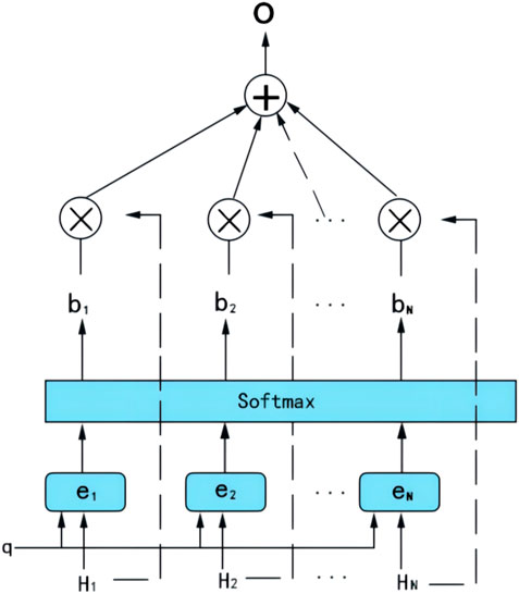
FIGURE 1. Attention mechanism based on the time sequence.

The similarity score $e_i$ between H_N and the output of hidden layer of each time step $H_i$ is calculated:

$e_i=Dot\left(\left.H_i,H_N\right]\right).(1)$

The importance of each time series node to the prediction result is different. Therefore, the state value of the hidden layer at the i-th time step and the state value of the final N-th time step are used to perform the dot product operation. A larger the result of the dot product operation indicates a stronger association between the time series node and the final predicted value.

Then, the Softmax function is employed for normalization to calculate the focus probability $b_i$ of the input sequence at the i-th time step:

$b_i=e_i/\left({\displaystyle \sum _{j=1}^N}{e}_j\right).(2)$

Last, the attention weight $b_i$ is multiplied by the corresponding hidden state value to obtain the output vector O of the attention layer:

$C={\displaystyle \sum _{j=1}^N}{b}_j \ast H_j.(3)$

The vector O is transferred to the fully-connected layer of the model to reach the final forecasting result.

2.3 BiGRU model

2.3.1 GRU model

The recurrent neural network (RNN) can create connections, i.e., short-term memories, between adjacent samples in a time sequence. When the input sequence is long, however, the problem of the vanishing gradient emerges, the long-distance dependence relations cannot be learned.

As a variant of RNN, the long short-term memory (LSTM) model improves the RNN by introducing selective memory and unit gates. LSTM solves the problem of the vanishing gradient that haunts RNNs and can learn long-term dependence relations in the sample data. Non-etheless, the LSTM network has complex structures and lots of parameters.

The GRU model is an improved variant of LSTM, with update gates and reset gates. Compared with LSTM, the GRU has less parameters and a more simplistic structure, which allows the parameters to converge quicklier and reduces the risks of overfitting.

Figure 2 shows the GRU neuron structure model.

FIGURE 2

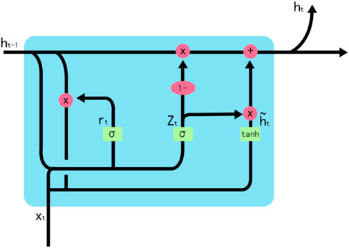
FIGURE 2. GRU neuron structure model.

The update gate in the GRU is defined as follows:

$z_t=\sigma \left(W_z \ast \left[x_t,h_{t-1}\right]\right),(4)$

where $x_t$ is the input vector of the t-th time step; $W_z$ is the weight matrix of the update gate; and $h_{t-1}$ is the output of the previous time step. The gated signal of the update gate is within 0 and 1, and a value closer to 1 indicates more past information being memorized.

The reset gate is defined as follows:

$r_t=\sigma \left(W_r \ast \left[x_t,h_{t-1}\right]\right),(5)$

where $W_r$ is the reset weight matrix. The reset gate is used to control the neglect of information in the previous time point. The obtained information after resetting is $h_{t-1}^{\prime }$:

$h_{t-1}^{\prime }=h_{t-1}\otimes r_t.(6)$

Then, the current cell state $\stackrel{\sim }{h_t}$ is calculated. The current cell state means selective memorization of the screened information and the current input, where $\otimes$ means multiplying the corresponding positions in two matrices or vectors, tanh is the activation function, and W is the weight:

$\stackrel{\sim }{h_t}=\tanh (W \ast \left[{x_t,h^{\prime }}_{t-1}\right].(7)$

The current output is $h_t$, and the vector will retain the current cell information and transfer it to the next cell:

$h_t={\left(1-z_t\right)\otimes h}_{t-1}+z_t\otimes \stackrel{\sim }{h_t.}(8)$

The final output of the current cell is:

$y_t={\sigma (W}_0 \ast h_t),(9)$

where ${\mathrm{W}}_0$ is the weight matrix.

2.3.2 BiGRU model

In a conventional GRU, information in the time sequence is transferred in a forward direction, the information far away from the current sequence suffers substantial attenuation, and the time-series information in the context is not considered. In a BiGRU model, two GRU running in opposite directions are trained (Lu and Duan, 2017). A BiGRU model combines two single-directional GRU, and the model output is determined by these two GRU. If the output of the forward GRU is $\overrightarrow{h_t}$, and the output of the backward GRU is $\stackrel{⃖}{h_t}$, then the output of the BiGRU is as follows:

$h_t=\overrightarrow{h_t}\oplus \stackrel{⃖}{h_t}(10)$

Figure 3 shows the structure of a BiGRU model, in which $\left\{h_1\to h_2\to \dots \to h_{\mathrm{n}}\right\}$ represents the hidden state sequence produced by the forward GRU, whereas $\left\{h_{\mathrm{n}}\to \dots h_2\to \to h_1\right\}$ is the hidden state sequence generated by the backward GRU.

FIGURE 3

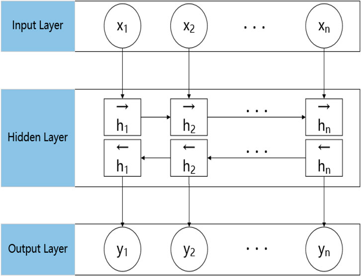
FIGURE 3. Structure of a BiGRU model.

2.4 Temporal convolutional neural networks

Bai et al. (Bai et al., 2018) proposed the temporal convolutional network (TCN) adding causal convolution and dilated convolution and using residual connections between each network layer to extract sequence features while avoiding gradient disappearance or explosion. A temporal convolutional network is essentially a deformation of one-dimensional convolution, which can be used for prediction of both temporal and textual data, and can achieve better results than recurrent neural networks for some tasks. Its layered structure of TCN is shown in Figure 4.

FIGURE 4

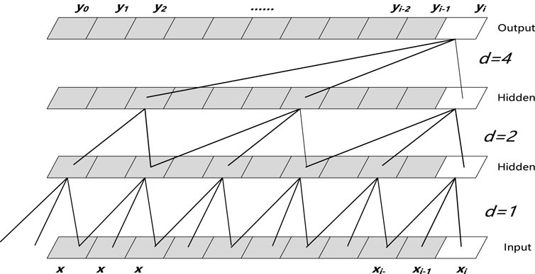
FIGURE 4. TCN network structure.

In Figure 4, $x_t$ indicates the input temporal data, ${\mathrm{y}}_t$ indicates the predicted values, and d indicates the size of the voids for the dilated convolution of each layer. The temporal convolutional network has two new operations compared with the ordinary 1-D convolutional network.

2.4.1 Causal convolution

The causal convolution strictly requires that only the information before the current moment to be predicted can be used to predict the current value, i.e., the information of the current moment is calculated based on $x_1$… $x_{t-1}$ and the current moment input $x_t$, which is calculated as follows.

$\mathrm{P}\left(x\right)={\displaystyle \prod _{\mathrm{t}=1}^{\mathrm{T}}}\mathrm{p}\left(x_t|x_1,x_2,...x_{\mathrm{t}-1}\right).(11)$

This ensures that information after the current moment is not involved in the calculation, and the historical information is not missed as in traditional CNN networks. Thus, the prediction of the temporal data is improved.

2.4.2 Dilated convolution

Dilated convolution is also called null convolution. In order to increase the perceptual field of convolution, it is necessary to increase the number of layers or the size of a very large filter, which is also a problem of causal convolution. Dilated convolution, on the other hand, expands the field of perception by skipping some of the inputs, which is equivalent to adding d zeros (d is the number of holes) between the elements of the convolution kernel, disguisedly expanding the size of the convolution kernel. The size of the convolution kernel after adding the dilation convolution is:

$f_{k\_d}=\left(d-l\right)\ast \left(f_k-l\right)+f_k,(12)$

where $f_k$ denotes the convolutional kernel size of the current layer. Since it can be computed in parallel, the computational efficiency of the model is lower than that of an ordinary convolutional network.

In addition, in order to make the sensory field increase and learn text features of larger lengths, the number of network layers is increased by expanding the convolution. However, an excessive increase in the number of network layers may incur the problem of gradient disappearance, and to solve this problem, residual links are introduced in the network structure.

2.5 WT-BiGRU-Attention-TCN model

Figure 5 shows the workflow of the WT-BiGRU-Attention-TCN model proposed in the present work.

FIGURE 5

FIGURE 5. Workflow of our WT-BiGRU-Attention-TCN model.

The proposed model is applied to wind power forecasting. The four methods (WT, BiGRU, Attention, TCN) in the model are used to solve problems at different stages of prediction: the wavelet transform is mainly used for data denoising at the data cleaning stage, while the other three methods are related to temporal feature extraction, including contextual feature extraction, feature weight calculation, and higher-level feature capturing. The methods are related by the data flow to form the framework of our model. The specific working process of the model is described below. First, the WT method is employed to denoise the dataset, and all sample features are normalized. Second, the BiGRU model is used to extract forward and backward features of the time-sequence data. Third, the weight of output information at each historical time sequence node is calculated by the time-sequence attention layer. Then, the hidden state output of the current state after adjustment is calculated based on the weight. Then, the TCN is used to obtain higher-level temporal features through causal and dilation convolution. Finally, the hidden state outputs by the TCN layer are input to the fully connected layer to obtain the forecasting result. The hierarchical structure and parameters of the model are shown in Table 1.

TABLE 1

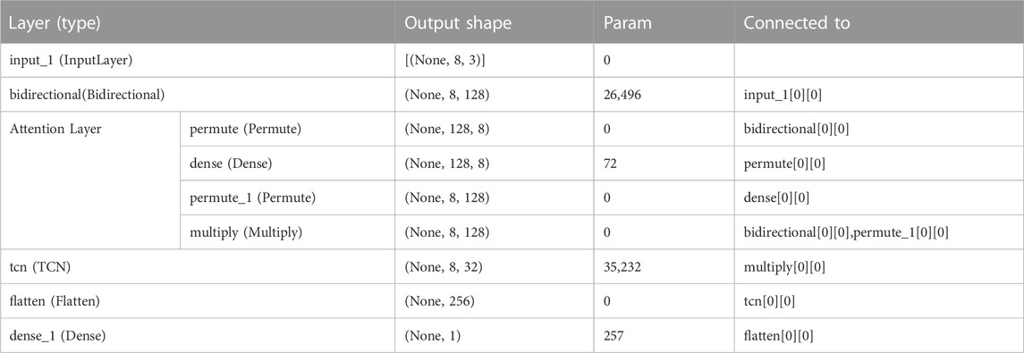
TABLE 1. The hierarchical structure and parameter information of our proposed model.

The input layer of the proposed model has a data dimension of (8,3) for each batch, i.e., the time step is 8 and the number of sample features is 3. The input data are combined by the GRU in both forward and backward propagation directions of the bidirectional layer, and the features learned by the two one-way GRU are stitched together to generate the set of vectors as the input of the attention layer. The attention layer calculates the generated weight vector for each time step and obtains the output of the attention layer by multiplying the weight vector with the output vector of the BiGRU layer. The vector generated by the attention layer is input to the TCN layer, and the field-of-perception size of the convolution is expanded to extract higher-level features by setting multiple expansion and causal convolution layers. The TCN output vector is subjected to the flatten operation to obtain the vector C. The vector C is then passed through the fully connected layer to obtain the value of the predicted wind power.

3 Experiment and analysis

3.1 Sample data

The wind power data used here are from the Galicia Wind Power Plant in northwestern Spain. A total of 52,123 pieces of valid data (from 1 January 2016 to 31 December 2016) were collected, with a sampling interval of 10 min. The features include meteorological indicators like wind speed and wind direction. Table 2 shows the specifics of the collected data, where WS represents the wind speed, DIR represents the wind direction, POWER represents the wind power, which is the target forecasting feature (the same applies to other tables and figures throughout this article).

TABLE 2

TABLE 2. Descriptive indicators for sample data.

As Table 2 shows, the sample data consists of three features. As these features have different dimensions and are substantially different from each other, normalization is required in the data preprocessing stage. The coefficient of variation of the feature “POWER” reaches 128.26%, which means large fluctuations of the wind power with time.

3.2 Data preprocessing

Data preprocessing mainly includes normalization of sample data and data denoising based on wavelet transform.

3.2.1 Data normalization

As the features of the data, including wind speed, wind direction and power, have different dimensions and show considerable differences in their range of value, normalization was performed to preclude the impact of the differences on the forecast result. Specifically, the values of the features were adjusted to a given range by min-max normalization, and the feature values were converted into a range of [0, 1]. The equation for min-max normalization is as follows:

$x_t^{\prime }=\frac{\left(x_t-x_{\mathit{min}}\right)}{\left(x_{\mathit{max}}-x_{\mathit{min}}\right)},(13)$

where $x_{\mathit{max}}$ and $x_{\mathit{min}}$ represent the maximum and the minimum of the same feature; $x_t$ represents the sample input data and $x_t^{\prime }$ represents the data after normalization.

3.2.2 Data denoising

There are inevitably noises in the sample data of wind power because of system error, random error, or human error, making it is imperative to perform data denoising. In the present work, the wavelet soft-thresholding method was employed. Specifically, with the valid information in the sample maintained, the wavelet decomposition was performed on the sample dataset, and thresholding was used to process the decomposed wavelet coefficient; then, wavelet reconstruction of the signals was performed to reduce the noise. The layers of the wavelet decomposition were set at 3, the global soft-thresholding was adopted, with a threshold set at 0.004. Three wavelet functions were employed to denoise the sample data. Table 3 shows denoising effects of the three feature variables by different wavelet functions.

TABLE 3

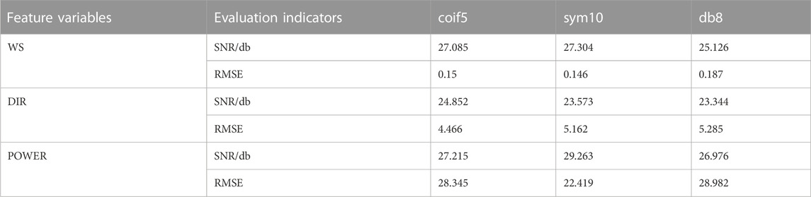
TABLE 3. Denoising effects of the three feature variables by different wavelet functions.

By the two evaluation indicators—SNR and RMSE, the most suitable denoising wavelet function for each feature variable was identified. Specifically, the function that reaches a higher SNR and a smaller RMSE would be selected. Finally, the appropriate wavelet function was selected for each feature: the sym10 function for WS and POWER, and the coif5 function for DIR.

Each feature variable was denoised by the selected wavelet functions. Figure 6 compares the curves of the three features before and after denoising.

FIGURE 6

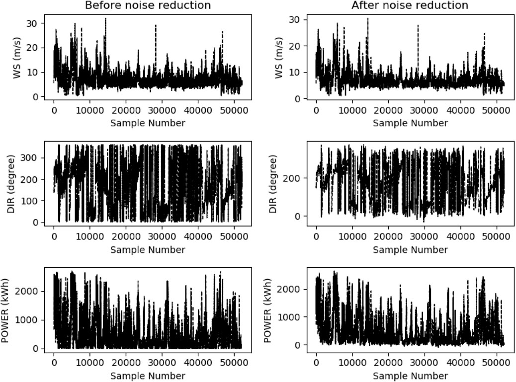
FIGURE 6. Comparison of the three feature variables before and after denoising.

As Figure 6 shows, the curves of denoised features have a high fitting precision with the curves of the original signals, which manifests the good smoothing effect of WT-based denoising. The denoising worked particularly well on the two features, “wind speed” and “power, which showed substantial fluctuations before denoising. Denoising has improved the SNR and reduced the noises of these two features, achieving a good smoothing effect on their curves, which alleviated the impact of abnormal values on the forecasting accuracy.

3.3 Model evaluation indicators

The sample data after data processing were transferred to the attention-based BiGRU network for model training. The GRU model was optimized based on the Adam algorithm (Kingma and Ba, 2014) by using an adaptive learning rate to effectively update the network weights. The Adam algorithm combines the advantages of Adagrad in dealing with sparse gradients and RMSProp in dealing with non-stationary targets, and calculates different adaptive learning rates for different parameters.

To measure the deviation between the predicted value and the actual value, we used root mean square error (RMSE) as the performance evaluation index of wind power forecasting. The root mean square error is the arithmetic square root of the mean square error (MSE). The calculation formula of the RMSE is shown in Eq. 14, where y_i is the true value, and p_i is the predicted value.

$\mathrm{R}\mathrm{M}\mathrm{S}\mathrm{E}=\sqrt{\frac{1}{N}{\displaystyle \sum _{i=1}^N}{\left(y_i-p_i\right)}^2}.(14)$

Two evaluation indicators, the mean absolute percentage error (MAPE) and R², were employed to assess the model’s forecast precision and fitting effect. MAPE indicates the absolute percentage errors of forecasts, and the closer the MAPE is to 0, the more accurate the model is. MAPE can be obtained by Eq. 15:

$\mathrm{M}\mathrm{A}\mathrm{P}\mathrm{E}=\frac{1}{N}{\displaystyle \sum _{i=1}^N}\frac{\left|y_i-{\widehat{y}}_i\right|}{\left|y_i\right|},(15)$

where ${\widehat{y}}_i$ is the predicted value, and y_i is the actual value.

R², which is known as the goodness of fit, indicates the percentage of variations in the dependent variables caused by the changes in the independent variable. It describes the fitting effect of the model, and is within a range of [0, 1]. A larger R² indicates a better fitting effect. The coefficient of determination can be calculated by Eq. 16:

${\mathrm{R}}^2=1-\frac{{\sum }_{i=1}^N{\left(y_i-{\widehat{y}}_i\right)}^2}{{\sum }_{i=1}^N{\left(y_i-{\overline{y}}_i\right)}^2},(16)$

where ${\widehat{y}}_i$ is the predicted value, and y_i is the actual value.

3.4 Comparative experiments and discussions

Our proposed model was compared with LSTM, GRU, WT-GRU, WT-BiGRU-Attention models to verify its superiority. The settings of the experiment are as follows: the time step of GRU and LSTM was set to 8 and the number of hidden units was 64. The convolutional kernel size of the TCN network was 3, the number of convolutional layers was 6, the list of expansion coefficients was (Liu et al., 2015a; Liu et al., 2015b; Wang et al., 2018; Han et al., 2019a; Ma et al., 2019a; Liu et al., 2022b), the number of filters used in the convolutional layers was 32, and relu was used as the activation function. The batch size of the prediction model was set to 100 and the epoch time was set to 50. Eighty percent of the total sample data was used as the training set and the remaining 20% was used as the test set. Table 3 shows the experiment result.

As Table 4 shows, the difference between the GRU model and the LSTM model in the two evaluation metrics of RMSE and R² is very small, which indicates that the prediction accuracy and the fitting effect of both are comparable. The prediction time used for the two models in the test set in the experiments is 1.37 s and 1.57 s, respectively, which means that the GRU operation efficiency is improved by 12.74% compared to LSTM. The reason is that the GRU model is more simplified and has fewer parameters than the LSTM model, and the model runs more efficiently. Therefore, the GRU model is considered as the base model in the combined model of our work, which can be applied to larger-scale data prediction.

TABLE 4

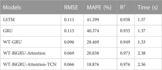
TABLE 4. Comparative experimental results of each model.

The comparison between WT-GRU and the conventional GRU model clearly shows that the model with a denoising module (WT-GRU) achieves a higher precision and accuracy than the one without. Specifically, WT-GRU reduces the RMSE by 0.019, which means it improves the forecasting precision by 16.52%; it achieves a significantly lower MAPE (29.49% lower than that achieved by the conventional GRU), which suggests the WT-GRU model has substantially improved the forecasting accuracy. The WT-GRU model has also increased the R² from 0.935 to 0.949, suggesting that it has improved the fitting effect by 1.5%. Figure 7 displays the fitting effect of the two models.

FIGURE 7

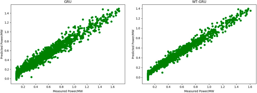
FIGURE 7. Fitting curves of true and predicted values of WT-GRU model and conventional GRU model.

As Figure 7 shows, after denoising, the curve of predicted power has a better fitting effect with the measured power curve, indicating that denoising can significantly improve the model’s forecasting performance. Experiments show that there is a certain amount of noise data in the wind power generation data samples, which will affect the effect of the prediction model. It is necessary to de-noise the data through wavelet transform.

Compared with WT-GRU, the WT-BiGRU-Attention model achieves an RMSE that is 0.027 lower, which means a 28.13% increase in the precision of prediction. Moreover, it achieves an MAPE that is 7.63% smaller and reaches an R² of 0.973, which means it has also improved the fitting effect. Although the WT-BiGRU-Attention model takes 1.01 s more prediction time than the GRU model on the full test set, its overall performance and efficiency is better. Figure 8 shows the fitting effect of the curve of predicted power achieved by WT-GRU and WT-BiGRU-Attention with the curve of the measured power.

FIGURE 8

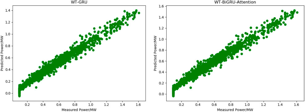
FIGURE 8. Fitting curves of measured and predicted power by WT-GRU model and WT-BiGRU-Attention model.

As shown in Figure 8, the WT-BiGRU-Attention achieves a better fitting effect than the WT-GRU. And according to the indicators in Table 4, we can find that the use of bi-directional GRU combined with temporal attention can improve the prediction accuracy of the traditional GRU model because bi-directional GRU is able to extract the forward and backward features of the sample data, and the attention mechanism enables the model to capture the features of key nodes in the time series and assign higher weights to these nodes, thus improving the prediction accuracy and the fitting effect of the model.

Figure 9 shows the fitting effect of forecasting power curves achieved by WT-BiGRU-Attention and our model with the measured power curve.

FIGURE 9

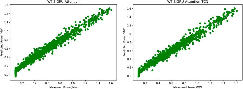
FIGURE 9. Fitting curves of measured and predicted power by WT-BiGRU-Attention and our model.

Figure 9 shows our model has further improved the fitting effect of the WT-BiGRU-Attention model. According to Table 4, though our model shares similar time for prediction to the WT-BiGRU-Attention model, it has reduced the RMSE by 4.35% and the MAPE by 9.42%, and improves the R² from 0.973 to 0.976. These statistics indicate that the TCN layer has further improved the accuracy of prediction. The TCN can make fullest of causal convolution and dilation convolution to obtain more higher-level temporal features, thus improving the model’s performance. As Table 4 shows, our model has the best performance overall.

4 Conclusion

Wind power is characterized by random fluctuations and is susceptible to impacts from various factors. Based on these characteristics, a new method termed WT-BiGRU-Attention-TCN model is proposed in the present work for wind power prediction. Experiments were made to compare its performance with other models, and the following conclusions were reached.

(1) The GRU model shows little difference from the LSTM model in terms of the fitting effect and forecasting precision, and the prediction performance of LSTM is slightly higher. However, they are considerably different in the model training and forecasting efficiency: the GRU model reduces the running time by 15.45%, suggesting that the GRU model is more suitable to forecasting tasks with large quantities of data. Thus, the GRU model is used as the fundamental model in the combination of models in our proposed method.

(2) The model that incorporates the wavelet transform-based denoising technique (WT-GRU) achieves higher forecasting accuracy than the traditional GRU model. WT-GRU also reaches a higher coefficient of determination (R²), indicating that introduction of the denoising module can significantly improve the model’s forecasting performance.

(3) The bidirectional GRU can extract both forward and backward features in the time sequence, thus outperforming the conventional GRU model. Moreover, by incorporating the attention mechanism, the model can capture the information of key nodes in the historical time steps and hence achieve higher precision.

(4) The temporal convolutional network (TCN) is used to obtain more higher-level temporal features through causal and dilation convolution. At the same time, its residual link structure is used to avoid the problem of gradient disappearance that may be caused by the excessive increase in the number of network layers. Thus, the TCN network can further improve the accuracy of the model.

In conclusion, with all evaluation indicators considered, our WT-BiGRU-Attention-TCN model performs best among all models compared in the present work. The model provides a new solution to high-precision forecasting of wind power generation.

Data availability statement

The original contributions presented in the study are included in the article/Supplementary Material, further inquiries can be directed to the corresponding author.

Author contributions

Conceptualization, DC; Methodology, DC; Software, DC; Validation, DC; Investigation, DC; Writing—original draft preparation, DC; Writing—review and editing, DC; Visualization, CY; Supervision, DC. All authors have read and agreed to the published version of the manuscript.

Conflict of interest

The authors declare that the research was conducted in the absence of any commercial or financial relationships that could be construed as a potential conflict of interest.

Publisher’s note

All claims expressed in this article are solely those of the authors and do not necessarily represent those of their affiliated organizations, or those of the publisher, the editors and the reviewers. Any product that may be evaluated in this article, or claim that may be made by its manufacturer, is not guaranteed or endorsed by the publisher.

References

Bai, S., Kolter, J. Z., and Koltun, V. (2018). An empirical evaluation of generic convolutional and recurrent networks for sequence modeling. https://arxiv.org/abs/1803.01271, arXiv preprint arXiv: 1803. 01271.

Google Scholar

Dang, D., Zhang, S., Ge, P., and Tian, X. (2019). Transformer fault diagnosis method based on improved quantum particle swarm optimization support vector machine. J. Electr. Power Sci. Technol. 34 (3), 6. CNKI:SUN:CSDL.0.2019-03-012.

Google Scholar

Ding, M., Zhou, H., Xie, H., Wu, M., Nakanishi, Y., and Yokoyama, R. (2019). A gated recurrent unit neural networks based wind speed error correction model for short-term wind power forecasting. Neurocomputing 365 (Nov.6), 54–61. doi:10.1016/j.neucom.2019.07.058

CrossRef Full Text | Google Scholar

Dong, X., Ning, X., Xu, J., Yu, L., Li, W., and Zhang, L. (2023). PFAS contamination: Pathway from communication to behavioral outcomes. IEEE Trans. Comput. Soc. Syst., 1–13. doi:10.1080/10810730.2023.2193144

CrossRef Full Text | Google Scholar

Duan, J., Wang, P., Ma, W., Tian, X., Liu, H., Cheng, Y., et al. (2021). Short-term wind power forecasting using the hybrid model of improved variational mode decomposition and correntropy long short -term memory neural network. Energy 214, 118980. doi:10.1016/j.energy.2020.118980

CrossRef Full Text | Google Scholar

Haigesa, R., Wanga, Y. D., Ghoshrayb, A., and Roskillya, A. P. (2017). Forecasting electricity generation capacity in Malaysia: An auto regressive integrated moving average approach. Energy Procedia 105, 3471–3478. doi:10.1016/j.egypro.2017.03.795

CrossRef Full Text | Google Scholar

Han, L., Jing, H., Zhang, R., and Gao, Z. (2019). Wind power forecast based on improved long short term memory network. Energy 189, 116300. doi:10.1016/j.energy.2019.116300

CrossRef Full Text | Google Scholar

Han, Z., Jing, G., Zhang, Y., Bai, R., Guo, K., and Zhang, Y. (2019). A review of wind power forecasting methods and new trends. Power Syst. Prot. Control 47 (24), 10. CNKI:SUN:JDQW.0.2019-24-023.

Google Scholar

Huang, X., Yu, H., Gong, X., and Liu, A. (2020). Wind power short-term prediction based on pso-ga-svm. Electr. Eng. 2020 (6), 4. CNKI:SUN:DGJY.0.2020-06-014.

Google Scholar

Kingma, D., and Ba, J. (2014). Adam: a method for stochastic optimization. Comput. Sci. [Preprint]. doi:10.48550/arXiv.1412.6980

CrossRef Full Text | Google Scholar

Korprasertsak, N., and Leephakpreeda, T. (2019). Robust short-term prediction of wind power generation under uncertainty via statistical interpretation of multiple forecasting models. Energy 180 (AUG.1), 387–397. doi:10.1016/j.energy.2019.05.101

CrossRef Full Text | Google Scholar

Li, D., and Li, Y. (2021). Ultra short term wind power prediction based on Deep learning and error correction. J. Sol. Energy 42 (12), 200–205. doi:10.19912/j.0254-0096.tynxb.2019-1464

CrossRef Full Text | Google Scholar

Li, L. (2007). The generation, development and application of wavelet analysis. China Water Transp. Theor. Ed. 5 (3), 96–98. CNKI:SUN:ZYUN.0.2007-03-044.

Google Scholar

Li, L., and Ye, L. (2010). Short-term wind power prediction based on improved persistence method. Trans. Chin. Soc. Agric. Eng. 26 (012), 182–187. doi:10.3969/j.issn.1002-6819.2010.12.031

CrossRef Full Text | Google Scholar

Liao, X., Wu, J., and Chen, C. (2022). Short-term wind power prediction model combining attention mechanism and lstm. Comput. Eng. 9, 048. doi:10.19678/j.issn.1000-3428.0062059

CrossRef Full Text | Google Scholar

Liu, D., Wang, J., and Wang, H. (2015). Short-term wind speed forecasting based on spectral clustering and optimised echo state networks. Renew. Energy 78, 599–608. doi:10.1016/j.renene.2015.01.022

CrossRef Full Text | Google Scholar

Liu, H., Tian, H. Q., and Li, Y. F. (2015). An emd-recursive arima method to predict wind speed for railway strong wind warning system. J. Wind Eng. Industrial Aerodynamics 141, 27–38. doi:10.1016/j.jweia.2015.02.004

CrossRef Full Text | Google Scholar

Liu, H., and Zhang, Z. (2022). A bilateral branch learning paradigm for short term wind power prediction with data of multiple sampling resolutions. J. Clean. Prod. 380 (1). 134977. doi:10.1016/j.jclepro.2022.134977

CrossRef Full Text | Google Scholar

Liu, X., Mo, Y., Wu, Z., and Yan, K. (2022). Hybrid deep learning model for ultra - short - term wind power prediction. J. Overseas Chin. Univ. Nat. Sci. Ed. 43 (5), 043.

Google Scholar

Liu, X., Yang, L., and Zhang, Z. (2022). The attention-assisted ordinary differential equation networks for short-term probabilistic wind power predictions. Appl. Energy 324, 119794. doi:10.1016/j.apenergy.2022.119794

CrossRef Full Text | Google Scholar

Liu, X., Zhou, J., and Qian, H. (2021). Short-term wind power forecasting by stacked recurrent neural networks with parametric sine activation function. Electr. Power Syst. Res. 192 (4), 107011. doi:10.1016/j.epsr.2020.107011

CrossRef Full Text | Google Scholar

Lu, P., Ye, L., Pei, M., He, B., Tang, Y., Zhai, B., et al. (2021). Optimization of GRACE risk stratification by N-terminal pro-B-type natriuretic peptide combined with D-dimer in patients with non-ST-elevation myocardial infarction. Proc. CSEE 41 (17), 13–19. doi:10.1016/j.amjcard.2020.10.050

CrossRef Full Text | Google Scholar

Lu, P., Ye, L., Zhong, W., Qu, Y., Zhai, B., Tang, Y., et al. (2020). A novel spatio-temporal wind power forecasting framework based on multi-output support vector machine and optimization strategy. J. Clean. Prod. 254, 119993. doi:10.1016/j.jclepro.2020.119993

CrossRef Full Text | Google Scholar

Lu, R., and Duan, Z. (2017). “Bidirectional GRU for sound event detection,” in Detection and Classification of Acoustic Scenes and Events (DCASE), 1–3.

Google Scholar

Ma, T., Wang, C., Peng, L., Guo, X., and Fu, Ming. (2019). Short term load forecasting of power system including demand response and deep structure multitasking learning. Electr. Meas. Instrum. 56 (16), 11. doi:10.19753/j.issn1001-1390.2019.016.009

CrossRef Full Text | Google Scholar

Ma, W., Cheng, R., Shi, J., Hua, Dong., Sun, G., and Zhang, C. (2019). Affine interval power flow calculation considering wind farm model. Guangdong Electr. Power 32 (11), 10. doi:10.3969/j.issn.1007-290X.2019.011.004

CrossRef Full Text | Google Scholar

Ning, X., Tian, W., He, F., Bai, X., Sun, L., and Li, W. (2023). Hyper-sausage coverage function neuron model and learning algorithm for image classification. Pattern Recognit. 136, 109216. doi:10.1016/j.patcog.2022.109216

CrossRef Full Text | Google Scholar

Niu, Z., Yu, Z., Li, B., and Tang, W. (2018). Short-term wind power prediction model based on depth-gated circulation unit neural network. Electr. Power Autom. Equip. 38 (5), 7. doi:10.16081/j.issn.1006-6047.2018.05.005

CrossRef Full Text | Google Scholar

Shahid, F., Zameer, A., and Muneeb, M. (2021). A novel genetic lstm model for wind power forecast. Energy 1, 120069. doi:10.1016/j.energy.2021.120069

CrossRef Full Text | Google Scholar

Shao, Z., Gao, F., Zhang, Q., and Yang, S. (2015). Multivariate statistical and similarity measure based semiparametric modeling of the probability distribution: A novel approach to the case study of mid-long term electricity consumption forecasting in China. Appl. Energy 156 (OCT.15), 502–518. doi:10.1016/j.apenergy.2015.07.037

CrossRef Full Text | Google Scholar

Sun, Y., Li, Z., Yu, X., Li, B., and Yang, M. (2020). Research on ultra-short-term wind power prediction considering source relevance. IEEE Access 8 (99), 147703–147710. doi:10.1109/ACCESS.2020.3012306

CrossRef Full Text | Google Scholar

Torres, J. L., Garcia, A., Blas, M. D., and Francisco, A. D. (2005). Forecast of hourly average wind speed with arma models in navarre (Spain). Sol. Energy 79 (1), 65–77. doi:10.1016/j.solener.2004.09.013

CrossRef Full Text | Google Scholar

Wang, T., Gao, J., Wang, Y., Shi, Z., Liu, T., Yang, B., et al. (2021). Research on wind power prediction based on improved empirical mode decomposition and support vector machine. Electr. Meas. Instrum. 58 (6), 6. doi:10.19753/j.issn1001-1390.2021.06.007

CrossRef Full Text | Google Scholar

Wang, Y., Wang, Y., Wang, L., and Chang, Q. (2018). Optimization of short-term load prediction model of neural network based on improved Drosophila algorithm. Electr. Meas. Instrum. 55 (22), 7. doi:10.3969/j.issn.1001-1390.2018.22.003

CrossRef Full Text | Google Scholar

Wu, J., Ding, M., and Zhang, J. (2018). Optimal allocation of wind farm energy storage capacity based on cloud model and k-means clustering. Automation Electr. Power Syst. 42 (24), 7. doi:10.7500/AEPS20180725007

CrossRef Full Text | Google Scholar

Yang, M., and Zhou, Y. (2019). Ultra-short-term prediction of wind power accounting for wind farm states. Chin. J. Electr. Eng. 39 (5), 10. CNKI:SUN:ZGDC.0.2019-05-001.

Google Scholar

Yu, R., Gao, J., Yu, M., Lu, W., Xu, T., Zhao, M., et al. (2018). Lstm-efg for wind power forecasting based on sequential correlation features. Future Gener. Comput. Syst. 93, 33–42. doi:10.1016/j.future.2018.09.054

CrossRef Full Text | Google Scholar

Zhao, H., and Guo, S. (2016). An optimized grey model for annual power load forecasting. Energy 107 (jul.15), 272–286. doi:10.1016/j.energy.2016.04.009

CrossRef Full Text | Google Scholar

Zhao, R., and Ding, Y. (2020). Short-term wind power prediction based on meemd-kelm. Electr. Meas. Instrum 57 (21), 7. doi:10.19753/j.issn1001-1390.2020.21.013

CrossRef Full Text | Google Scholar

Zn, A., Zy, A., Wt, A., Qw, A., and Mrb, C. Wind power forecasting using attention-based gated recurrent unit network. Energy 196. 117081. doi:10.1016/j.energy.2020.117081

CrossRef Full Text | Google Scholar