Bi-level energy management strategy for power-split plug-in hybrid electric vehicles: A reinforcement learning approach for prediction and control

The implementation of an energy management strategy plays a key role in improving the fuel economy of plug-in hybrid electric vehicles (PHEVs). In this article, a bi-level energy management strategy with a novel speed prediction method leveraged by reinforcement learning is proposed to construct the optimization scheme for the inner energy allocation of PHEVs. First, the powertrain transmission model of the PHEV in a power-split type is analyzed in detail to obtain the energy routing and its crucial characteristics. Second, a Q-learning (QL) algorithm is applied to establish the speed predictor. Third, the double QL algorithm is introduced to train an effective controller offline that realizes the optimal power distribution. Finally, given a reference battery's state of charge (SOC), a model predictive control framework solved by the reinforcement learning agent with a novel speed predictor is proposed to build the bi-level energy management strategy. The simulation results show that the proposed method performs with a satisfying fuel economy in different driving scenarios while tracking the corresponding SOC references. Moreover, the calculation performance also implies the potential online capability of the proposed method.

1 Introduction

The contradiction between energy shortage and the booming development of the automotive industry has been increasingly prominent in recent years. Vehicle electrification that substitutes fossil fuel with cleaner electrical energy has become a critical development trend in this field (Li et al., 2017). The plug-in hybrid electric vehicle (PHEV), which is widely known as a promising solution in new energy vehicles, takes the considerations of both driving range and energy saving. PHEVs contain two power sources, generally: the electricity stored in batteries or super-capacitors (as the primary power source) and fuel (as the secondary power source). Therefore, the PHEVs can coordinate the motor and engine according to their respective energy characteristics in complex driving conditions so as to avoid low operational efficiency that may lead to unnecessary energy consumption and emission (Biswas and Emadi, 2019). However, the effective conversion between the two different power sources is usually reflected as a time-varying and non-linear optimization problem that makes it difficult to design a general energy management strategy (EMS) for PHEVs, and the precise control of PHEV powertrain has become the focus of current academic research.

Currently, the EMS of PHEVs can be divided into two types: rule-based EMSs and optimization-based EMSs (Han et al., 2020). Among these, the rule-based EMSs are generally based on the experience of engineering implementation, and a series of control rules are preset to realize the energy distribution of the power system. The charge-depleting/charge-sustaining (CD/CS) strategy is the most widely used rule-based EMS (Overington and Rajakaruna, 2015). Taking advantage of the large battery capacity, in the CD mode, the battery serves as the unique power source that drives the vehicle. When the battery's state of charge (SOC) drops to a certain threshold, the strategy switches to the CS mode and the power for battery charging and vehicle driving is provided by the engine to ensure that the SOC runs near the threshold. However, there is an obvious downside to this strategy that with increasing driving mileage, the fuel economy worsens (Singh et al., 2021). Rule-based EMSs highly rely on engineering experience and find it difficult to adapt to various operating conditions while ensuring satisfactory fuel economy.

Optimization-based EMSs can be further classified into two categories: global optimization and instantaneous optimization. The global optimal EMS is featured as knowing the global information about the working conditions in advance and then allocating the optimal energy to the power source that can be solved by common algorithms such as the dynamic programming (DP) (Peng et al., 2017), Pontryagin’s minimum principle (PMP) (Chen et al., 2014), and game theory (GT) (Cheng et al., 2020). In Lei et al. (2020), DP is first applied to perform offline global optimization for a PHEV, and by combining the K-means clustering method, a hybrid strategy considering the driving conditions is proposed, which achieves a similar fuel economy to that of the DP. In Sun et al. (2021), the formal characteristics of the bus on a fixed section of a road are fully taken into account, while the authors propose a PMP algorithm that can be applied in real time to achieve near-optimal fuel economy. However, global optimization methods have a common characteristic of being too computationally intensive for online applications (Jeong et al., 2014). Thus, they are frequently employed as evaluation criteria for other methods or for extracting optimal control rules in general. The instantaneous optimization methods, such as the equivalent consumption minimization strategy (ECMS) (Zhang et al., 2020a; Chen et al., 2022a), model predictive control (MPC) (Guo et al., 2019; Ruan et al., 2022), and reinforcement learning (RL) (Chen et al., 2018; Zhang et al., 2020b), have become common approaches in solving energy management online application problems. The MPC method can effectively deal with multivariate constraint problems with strong robustness and stability and has been widely employed in control problems that are strongly non-linear (He et al., 2021). In Quan et al. (2021), a speed prediction MPC controller was developed, and on the basis of the Markov speed predictor, an exponential smoothing rate had been hired to modify the Markov speed predictor. In Zhang et al. (2020c), Markov and back propagation (BP) neural networks were engaged for speed prediction, and an EMS combined vehicle speed prediction based on the adaptive ECM strategy (AECMS) algorithm was presented, which could improve fuel economy by 3.7% when compared to the rule-based method. In Zhou et al. (2020a), a fuzzy C-mean clustering integrating Markov co-rate prediction had been exerted to regulate the battery's SOC rate under different conditions. In Guo et al. (2021a), a real-time predictive energy management strategy was proposed, a model predictive control problem was formulated, and numerical simulations were carried out all yielding a desirable performance of the proposed PEMS in fuel consumption minimization and battery aging restriction.

With the rapid development of artificial intelligence technology, RL has attracted much attention for its strong learning ability and real-time capability in tackling high-dimensional complex problems due to its unique learning behavior (Ganesh and Xu, 2022). Chen et al. (2020) proposed a stochastic MPC controller based on Markov’s speed prediction and Q-learning (QL) algorithm, which can achieve fuel economy similar to that of the stochastic DP (SDP) strategy. In Yang et al. (2021), considering the long-term nature of direct reinforcement learning training processes, an indirect learning EMS based on a higher-order Markov chain model was proposed.

Based on the abovementioned literature review, MPC and RL have been widely applied in the energy management of PHEVs. According to the authors’ knowledge, in the design EMS using MPC method, general speed prediction methods such as the Markov (Zhou et al., 2020b), neural network (Chen et al., 2022b), or combination (Lin et al., 2021; Liu et al., 2021). However, the RL algorithm is rarely applied in designing the speed prediction controller. In addition, considering that the RL feature regulates better and avoids the random error generated by the Markov and neural network methods in predicting vehicle speed, a bi-level EMS based on RL speed prediction is proposed in this study. The RL algorithm is adopted in the upper layer controller to establish the speed predictor, and the double QL algorithm is exercised in the lower layer to perform rolling optimization. Numerical simulations are conducted to validate and evaluate the fuel economy effect of the proposed method, and the computational efficiency and applicability of the proposed method on different reference trajectories are further analyzed. The main contributions of this study are as follows: 1) the speed prediction problem is solved by the RL method and 2) an RL controller combining RL velocity prediction and RL rolling optimization is established, which provides effective support for the online application of machine learning methods on PHEVs.

The remainder of this article is assigned as follows: Section 2 constructs the EMS objective function, and the powertrain structure of the PHEV is analyzed in detail by using the mathematical model. In Section 3, the speed predictor is established by QL, and its prediction accuracy is analyzed. In Section 4, the bi-level EMS framework is built, and the double QL controller is employed to carry out the rolling optimization process. Section 5 verifies the effectiveness, applicability, and practicality of the proposed method. Section 6 provides the conclusion of this study.

2 Modeling of PHEV

A power-split PHEV is taken as the research object in this study, of which the prototype model is the Toyota Prius. The powertrain transmission configuration of the PHEV is shown in Figure 1, which consists of an engine, a lithium-ion battery pack, two electric motors, a planetary gear power distribution unit, and two electrical energy converters. Thereinto, the engine is connected to the planet gear, motor 1 is connected to the ring gear, and motor 2 is connected to the sun gear. The planetary gear power distribution unit can make the engine, motor, and wheels operate without interfering with each other so as to realize the reasonable distribution of the driving force of the whole vehicle through the power coupling relationship. The detailed vehicle structure parameters are listed in Table 1.

FIGURE 1

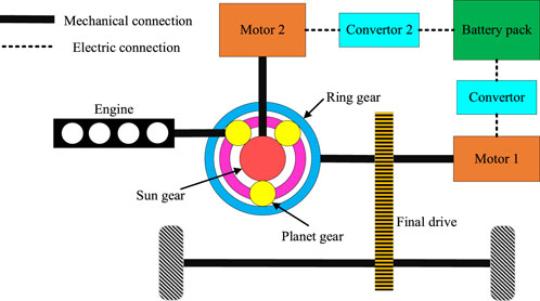
FIGURE 1. Powertrain transmission configuration of the PHEV.

TABLE 1

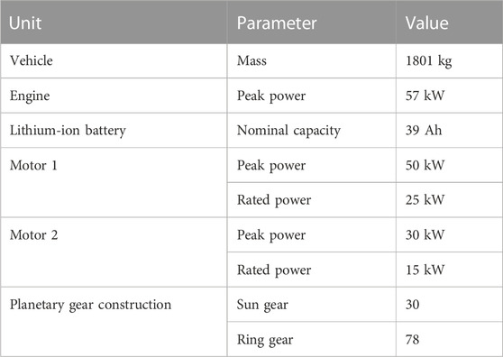
TABLE 1. Main parameters of the power-split PHEV.

In this article, the main objective is to rationalize the energy transfer relationship between the engine and battery such that the total fuel consumption of the vehicle in a driving cycle is minimized. The cost function can be expressed as

$J=\min Fue{l}_{total}=\min {\int }_0^{T}Fue{l}_{rate}dt,(1)$

$Fue{l}_{rate}=f\left({\omega }_{eng},{\mathrm{T}}_{eng}\right),(2)$

where $Fue{l}_{total}$ denotes the total fuel consumption during the whole driving cycle, $Fue{l}_{rate}$ indicates the instantaneous fuel consumption, $T$ represents the total time of the whole driving cycle, ${\omega }_{eng}$ stands for the engine speed, and $T_{eng}$ means the engine torque. In order to obtain the instantaneous fuel consumption of the PHEV, the energy demand model and energy flow relationship of the PHEV are analyzed.

In the study, the lateral dynamic effects of the vehicle are ignored, and the complex vehicle model is considered to be a simple quasi-static model. For a given driving condition, according to the longitudinal dynamics model of the vehicle, the power demand of the vehicle can be deduced as

$P_{drive}=\left(F_f+F_w+F_i+F_j\right)v,(3)$

where $P_{drive}$ indicates to the power demand of the vehicle; $F_f$, $F_i$, $F_w$, and $F_j$, respectively, signify the rolling resistance, grade resistance, air resistance, and acceleration resistance; and $v$ is the vehicle speed. The four types of resistances can be formulated as

$\left\{\begin{array}{l}{F}_f=mgf\cos \alpha \\ F_w=C_{d}A{v}^2/21.15\\ F_i=mg\sin \alpha \\ F_j=\delta ma\end{array}\right.,(4)$

where $m$ denotes vehicle mass, $g$ means gravitational acceleration, $f$ represents the rolling resistance coefficient, $\alpha$ indicates to the slope of travel, $C_d$ defines the air resistance coefficient, $A$ stands for the windward area of the vehicle, $\delta$ refers to the rotating mass conversion factor of the vehicle, and $a$ is the acceleration.

In integrating the PHEV energy transfer model as shown in Figure 1, the required power of the vehicle is provided by the engine and battery, and the battery drives two electric motors to provide kinetic energy, and the demand power is presented as

$\left\{\begin{array}{l}{P}_{drive}=P_{final}\cdot {\eta }_{final}\\ P_{final}=\left(P_{eng}+P_{ess}\right)\cdot {\eta }_{gear}\\ P_{ess}=\left(P_{mot1}/{\eta }_{mot1}+P_{mot2}/{\eta }_{mot2}\right)+P_{elec}\\ P_{ess}=\left(\left({\omega }_{mot1}\cdot T_{mot1}\right){\eta }_{mot1}+\left({\omega }_{mot2}\cdot T_{mot2}\right){\eta }_{mot2}\right)+P_{elec}\end{array}\right.,(5)$

where $P_{final}$, $P_{eng}$, $P_{ess}$, $P_{mot1}$, $P_{mot2}$, and $P_{elec}$ represent the power of the main gearbox, engine, battery, motor 1, motor 2, and electrical accessories, respectively. ${\eta }_{final}$, ${\eta }_{gear}$, ${\eta }_{mot1}$, and ${\eta }_{mot2}$ mean the transmission efficiency of the main reducer, transmission unit, motor 1, and motor 2, respectively. ${\omega }_{mot1}$ and ${\omega }_{mot2}$ denote the speed of motor 1 and motor 2, respectively. $T_{mot1}$ and $T_{mot2}$ stand for the torque of motor 1 and motor 2, respectively. Considering that the engine and the two motors work by means of a planetary gear unit, the coupling relationship can be expressed as

$\left\{\begin{array}{l}{\omega }_{eng}=\left(1/1+\mu \right){\omega }_{mot1}+\left(\mu /1+\mu \right){\omega }_{mot2}\\ T_{eng}=\left(1+\mu \right)T_{mot1}=\left(1+1/\mu \right)T_{mot2}\end{array}\right.,(6)$

where $\mu$ indicates the gear ratio of the planetary gear.

Eqs 2–6 reveal that the total fuel consumption of the vehicle throughout the driving cycle is decided by controlling the engine speed and torque. Considering that two control degrees of freedom—the speed and torque—increase the complexity of the control strategy, the engine optimal operating line (OOL), as shown in Figure 2, is engaged to constitute their mapping relationship and simplify the calculation process (Chen et al., 2015). Giving an engine power request, an optimal engine speed and, consequently, the optimal engine torque can be obtained. Thus, the fuel consumption rate of the engine at each moment can be determined through the engine fuel consumption rate map, as shown in Figure 3. The corresponding mathematical relationship can be exhibited as

${\omega }_{eng}=h^{\ast }\left(P_{eng}\right).(7)$

FIGURE 2

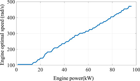
FIGURE 2. Engine optimal operating line.

FIGURE 3

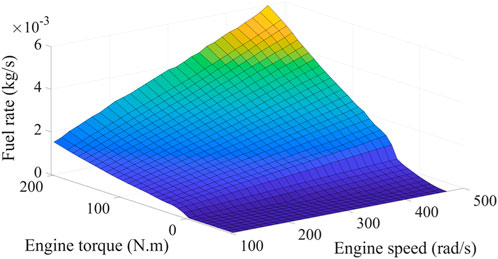
FIGURE 3. Engine fuel consumption rate MAP.

With the introduction of the engine OOL, it can be found from Eqs 2–7 that the instantaneous fuel consumption of the engine can be determined from the battery power, power demand, and vehicle speed, that is,

$f\left({\omega }_{eng},{\mathrm{T}}_{eng}\right)=f\left(P_{drive},P_{ess},v\right).(8)$

In this study, a simple equivalent circuit model that includes the internal resistance and open-circuit voltage is applied to characterize the performance of the battery as

$\left\{\begin{array}{l}{I}_{ess}=OCV-\frac{\sqrt{OC{V}^2-4R_{\mathrm{int}}{P}_{ess}}}{2R_{\mathrm{int}}}\\ P_{ess}=OCV\cdot I_{ess}-{I_{ess}}^2{R}_{\mathrm{int}},\\ SOC\left(t\right)=SO{C}_{init}-\frac{1}{C_{ess}{\int }_0^t{I}_{ess}dt}\end{array}\right.(9)$

where $I_{ess}$ is the battery current, $OCV$ denotes the open-circuit voltage, $R_{\mathrm{int}}$ represents the internal resistance, $SOC\left(t\right)$ indicates the $SOC$ value at time step t, $SO{C}_{init}$ means the initial $SOC$ value, and $C_{ess}$ stands for the battery capacity. In this equivalent circuit model, the open-circuit voltage and internal resistance are determined by the instantaneous SOC value, as shown in Figure 4. It can be found that when the SOC decreases, the open-circuit voltage decreases from 220 V to 165 V and internal resistance varies from 0.09 Ω to 0.14 Ω.

FIGURE 4

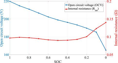
FIGURE 4. Variation of $OCV$ and $R_{\mathrm{int}}$ with the SOC.

According to the analysis mentioned above, it is found that instantaneous fuel consumption can be obtained when the battery power is determined. Therefore, in this study, battery power is applied as the control variable to obtain fuel consumption. Considering the power limitations and performance requirements of the PHEV, the following constraints also have to be made:

$\left\{\begin{array}{l}{P}_{\mathrm{d}\mathrm{r}\mathrm{i}\mathrm{v}\mathrm{e}\_\mathrm{m}\mathrm{i}\mathrm{n}}<P_{drive}<P_{\mathrm{d}\mathrm{r}\mathrm{i}\mathrm{v}\mathrm{e}\_\mathrm{m}\mathrm{a}\mathrm{x}}\\ P_{eng\_\mathrm{m}\mathrm{i}\mathrm{n}}<P_{eng}<P_{eng\_\mathrm{m}\mathrm{a}\mathrm{x}}\\ P_{\mathrm{e}\mathrm{s}\mathrm{s}\_\mathrm{m}\mathrm{i}\mathrm{n}}<P_{\mathrm{e}\mathrm{s}\mathrm{s}}<P_{ess\_\mathrm{m}\mathrm{a}\mathrm{x}}\\ P_{\mathrm{m}\mathrm{o}\mathrm{t}1\_\mathrm{m}\mathrm{i}\mathrm{n}}<P_{\mathrm{m}\mathrm{o}\mathrm{t}1}<P_{\mathrm{m}\mathrm{o}\mathrm{t}1\_\mathrm{m}\mathrm{a}\mathrm{x}}\\ P_{\mathrm{m}\mathrm{o}\mathrm{t}2\_\mathrm{m}\mathrm{i}\mathrm{n}}<P_{\mathrm{m}\mathrm{o}\mathrm{t}2}<P_{\mathrm{m}\mathrm{o}\mathrm{t}2\_\mathrm{m}\mathrm{a}\mathrm{x}}\\ SO{C}_{\min }<SOC<SO{C}_{\max }\end{array}\right.,(10)$

where the subscripts indicate the minimum and maximum values of the variables, respectively.

Based on the abovementioned energy flow analysis, a bi-level EMS based on RL speed prediction will be developed to determine the optimal battery power at each moment, which is described in detail in the Section 3.

3 Speed prediction based on QL

3.1 QL algorithm

As an important milestone of the RL algorithm, QL has been widely used in many fields due to its characteristics of efficient convergence and easy implementation (Watkins et al., 1992). The main idea of the QL algorithm is to form a value function $Q$ that can be directly iterated and updated by state–action pairs and update the value function $Q$ through the interaction between the agent and environment to obtain the optimal action strategy set under certain conditions. The QL algorithm can be summarized in a simple five-tuple representation $\left\{S,A,\gamma ,R,\pi \right\}$, where $S$ denotes the state variable, $A$ denotes the action variable, $R$ denotes the reward function, $\gamma$ denotes the discount factor of the agent in the learning process, and $\pi$ denotes the optimal action strategy set for the agent to interact with the environment.

In the QL algorithm, the agent is a learner and the decision maker, interacting with different states of the environment at each moment. The agent decides $a_t$ according to the current state $s_t$. After receiving the decision, the environment enters the new state $s_{t+1}$ and gives the corresponding reward $r_{t+1}$, and the agent continuously learns and improves its actions on the basis of the reward received until the maximum cumulative reward is obtained. The cumulative expected reward obtained by the agent in the learning process is known as the expectation function, and it can be described as

$V=E\left({\displaystyle \sum }_{t=0}^T{\gamma }^t{r}_t\right).(11)$

As future actions and states are unpredictable when the agent performs the current action, the state–action pair function $Q$ is introduced to estimate the expected future payoffs those result from the actions according to some future strategy in the currently known state. This can be expressed as

$Q\left(s,a\right)=r\left(s,a\right)+\gamma E_{\pi }\left[Q\left(s^{\prime },a^{\prime }\right)\right],(12)$

where $s^{\prime }$ denotes the next state, $a^{\prime }$ denotes the action corresponding to the next state, and after the learning task is accomplished by the agent, the optimal state–action pair function $Q^{\ast }\left(s,a\right)$ is obtained as

${\pi }^{\ast }=\underset{a\in A}{\mathrm{argmax}}{Q}^{\ast }\left(s,a\right).(13)$

During the learning process of the agent, the updated rule of the value function can be expressed as

$Q\left(s,a\right)\leftarrow Q\left(s,a\right)+\beta \left(r+\gamma \underset{a}{\max }Q\left(s^{\prime },a\right)-Q\left(s,a\right)\right),(14)$

where $\beta$ represents the learning efficiency. The greater the learning efficiency, the faster the convergence speed, but it should not be too large or otherwise it will lead to the problem of overfitting.

In Section 3.2, QL is employed for speed prediction in preparing the groundwork for bi-level energy management later on.

3.2 Speed prediction based on QL

In this study, the QL method is employed for speed prediction in the bi-level energy management framework. In the QL-based speed predictor, the state space, action space, and reward function of the controller system have to be determined first. The driving speed of the vehicle is taken as the state variable, and the vehicle speed is discretized into $m$ intervals, which can be expressed as

$S\in \left\{v_{spd}^1,v_{spd}^2,v_{spd}^3,\cdots ,v_{spd}^m\right\},(15)$

where $v_{spd}$ represents the current speed state. Moreover, the acceleration can be regarded as a random variable due to the strong uncertainty in the actual driving process of the vehicle. Therefore, the acceleration is taken as the control variable, and it ranges from $-4m/s^2$ to $4m/s^2$ and is discretized into $n$ intervals as

$A=\left\{a_{acc}^1,a_{acc}^2,a_{acc}^3,\cdots ,a_{acc}^n\right\}.(16)$

The instantaneous reward is set to the absolute value of the difference between the predicted vehicle speed and the actual value as

$v_{diff}\left(t\right)=\left|v_{pre}\left(t\right)-v_{real}\left(t\right)\right|,(17)$

where $v_{pre}\left(t\right)$ and $v_{real}\left(t\right)$, respectively, denote the predicted velocity and real velocity. The specific reward value is defined as

$r\left(t\right)=\left\{\begin{array}{ll}100& 0\le v_{diff}\le 0.25\\ 75& 0.25<v_{diff}\le 0.5\\ 50& 0.5<v_{diff}\le 1\\ 25& 1<v_{diff}\le 1.5\\ 0& 1.5<v_{diff}\le 2\\ -1000& v_{diff}>2\end{array}\right..(18)$

After setting the state space, action space, and reward function of the controller, five standard cycles: CLTCP, JC08, WLTC, LA92, and FTP75, as shown in Figure 5, are applied as the training cycle to train the QL speed prediction controller, and the number of iterations is set to 500. As can be seen from Figure 5, the five standard operating cycles cover a variety of speed segments, such as low speed, medium speed, high speed, and rapid acceleration/deceleration. Here, the QL is engaged to cover future speeds, and the iteration process is tabulated in Table 2. The cumulative reward of the QL velocity controller for different prediction time domains is depicted in Figure 6, where the cumulative reward gradually converges to a constant value as the number of iterations increases. Figure 7 shows the cumulative reward difference at each iteration process with different prediction time domains; similarly, the difference flattens out and gradually converges to a stable value as the number of iterations increases continuously. From this point on, we find that the QL speed controller gradually converges and stabilizes after 500 iterations of learning.

FIGURE 5

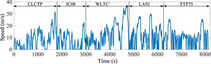
FIGURE 5. Training cycle.

TABLE 2

TABLE 2. Iterative process of the QL speed predictor.

FIGURE 6

FIGURE 6. Cumulative reward.

FIGURE 7

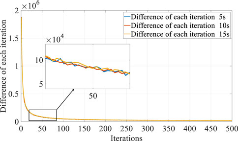
FIGURE 7. Cumulative reward difference for each iteration.

3.3 Contrast analysis

During the actual vehicle operation, the acceleration of the vehicle features strong uncertainty, which can be described as a discrete Markov chain model (Ganesh and Xu, 2022); therefore, the Markov chain model is applied as an ordinary method for speed prediction. To effectively validate the proposed speed prediction method, the prediction results based on the Markov chain model are compared. Note that the proposed method and the Markov chain model are trained with the same training data, and the UDDS, HWFET, NEDC, and WVUSUB cycles are each applied to test the models.

In addition, two different error functions—$Err$ and RMSE—are calculated to evaluate the speed prediction performance as

$\left\{\begin{array}{l}Err\left(t\right)=\sqrt{{\displaystyle \sum }_{i=1}^{t_p}{\left(v_{t,i}^{pre}-v_{t,i}^{real}\right)}^2/t_p}\\ RMSE={\displaystyle \sum }_{t=1}^{T}Err\left(t\right)/T\end{array}\right.,(19)$

where $Err\left(t\right)$ denotes the RMSE value of the predicted velocity series and actual velocity series in the predicted time domain at time $t$, $t_p$ represents the predicted time domain, $v_{t,i}^{pre}$ denotes the predicted speed at the $i‑th$ second after time $t$, $v_{t,i}^{real}$ represents the actual velocity at the $i‑th$ second after time $t$, and $T$ indicates the total duration of the working cycle.

The comparison results of the two velocity predictors with the prediction length varying within 3 s, 5 s, 10 s, and 15 s that are based on the UDDS cycle are shown in Figure 8, and the statistic errors are given in Table 3.

FIGURE 8

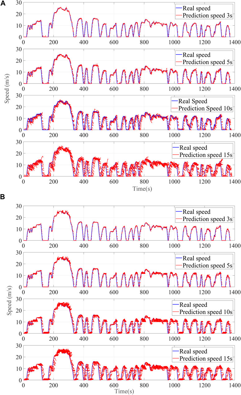
FIGURE 8. Comparison of speed prediction results: (A) Markov speed method and (B) QL speed method.

TABLE 3

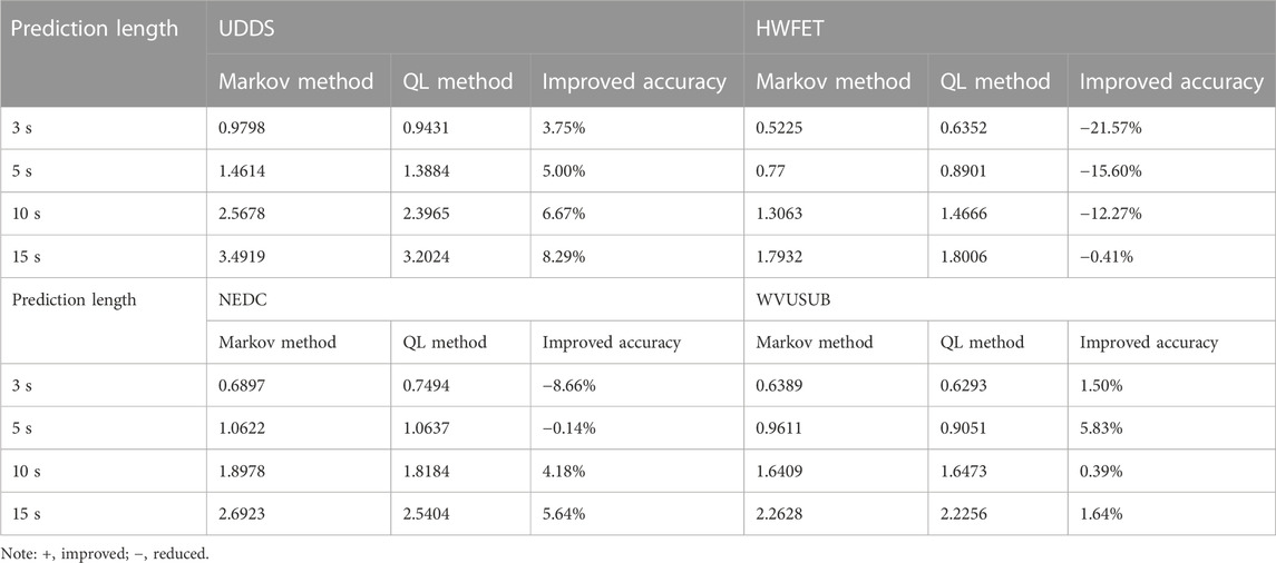
TABLE 3. Comparative analysis of speed prediction results.

It is noted from these comparison results that the Markov method is a random prediction method with different speed prediction values for each step, whereas the QL velocity prediction method is a highly regular prediction method with the same velocity prediction trajectory at different moments when the velocity value is in a certain state interval range. Therefore, the advantages of the QL speed prediction method can be obtained such that if the convergence of the QL training process can be guaranteed, the interference of the prediction accuracy caused by the randomness of speed prediction can be avoided.

In addition, Table 3 shows the RMSE indexes of the two methods. Taking the Markov method as the benchmark, it can be found that the prediction accuracy improves with the increase of prediction time, especially for high-speed conditions such as HWFET. Although the prediction accuracy is very low when compared with Markov speed prediction at 3 s, the prediction accuracy also improves with the prediction time, which can likewise indicate that the QL velocity prediction method can avoid the interference of prediction accuracy caused by the randomness of the prediction. Considering the influence of prediction duration on the design of EMS, the design prediction duration of bi-level energy management in the following is 10 s.

4 Bi-level energy management strategy

The MPC is a rolling optimization control algorithm implemented online that combines predictive information and a rolling optimization mechanism for better control of performance when dealing with non-linear models. The bi-level EMS designed in this study is shown in Figure 9. The upper controller is the speed prediction model developed in the section 3.2, of which the prediction length is 10 s; and the speed prediction results are input into the lower controller. In the lower controller, a valid and convergent double QL offline controller is trained first, and the SOC trajectory calculated by the double QL offline controller is treated as the reference trajectory of the MPC. Based on the prediction model of input vehicle speed information, the first sequence of the control sequences in the prediction time domain is output after correction by feedback. The double QL offline controller is first introduced as described in Section 4.1.

FIGURE 9

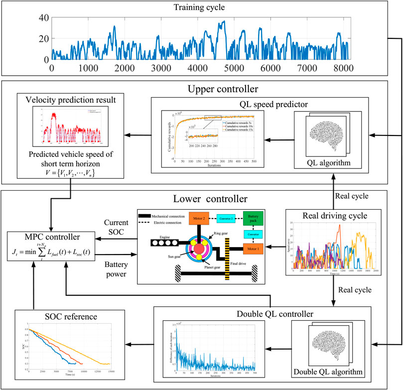
FIGURE 9. Framework of the bi-level EMS.

4.1 Double QL offline controller

The double QL algorithm is an improved QL algorithm proposed by Watkins et al. (1992). The double QL differs from the QL algorithm in employing two state–action pair functions to solve the optimal action according to Eq. 14. It is known that the update of the optimal value function $Q$ depends on $\max Q\left(s^{\prime },a\right)$, and the QL method updates the expected value by taking the maximum value of $Q$ before finding the expected value, which results in an overestimation of the action value to a large extent. Therefore, the double QL avoids overestimating the value function by constructing two Q functions and also ensures the iterative efficiency of the algorithm. To a certain extent, it can be considered that the double QL therefore achieves better results than the QL method.

In the double QL algorithm of this study, the power demand $P_{req}$ and battery $SOC$ are set as the state variables and can be discretized by $l$ and $p$ intervals. The battery power output $P_{ess}$ is set as an action variable and discretized into $k$ intervals, and the state variables and action variables of the algorithm are represented as

$\left\{\begin{array}{l}S\in \left\{\left(SO{C}^1,P_{req}^1\right),\left(SO{C}^1,P_{req}^2\right),\left(SO{C}^1,P_{req}^3\right),\cdots ,\left(SO{C}^p,P_{req}^l\right)\right\}\\ A=\left\{P_{ess}^1,P_{ess}^2,P_{ess}^3,\cdots ,P_{ess}^k\right\}\end{array}\right..(20)$

The instantaneous reward function $r\left(t\right)$ is judged by the engine’s on–off and $SOC$ values, and the specific reward function value is expressed as

$r\left(t\right)=\left\{\begin{array}{ll}-Fue{l}_{rate}\cdot {10}^6& eng\_on=1\cap 0.3\le SOC\le 0.9\\ \left(-Fue{l}_{rate}\cdot {10}^6\right)\cdot 10& eng\_on=1\cap \left(SOC<0.3|SOC>0.9\right)\\ 0.5/Fue{l}_{rate\_\mathrm{m}\mathrm{a}\mathrm{x}}& eng\_on=0\cap 0.3\le SOC<0.5\\ 1/Fue{l}_{rate\_\mathrm{m}\mathrm{a}\mathrm{x}}& eng\_on=0\cap 0.5\le SOC<0.7\\ 2/Fue{l}_{rate\_\mathrm{m}\mathrm{a}\mathrm{x}}& eng\_on=0\cap 0.7\le SOC<0.9\\ -2000& eng\_on=0\cap SOC<0.3\end{array}\right.,(21)$

where $eng\_on=1$ indicates that the engine is turned on, $eng\_on=0$ indicates that the engine is turned off. $Fue{l}_{rate\_\mathrm{m}\mathrm{a}\mathrm{x}}$ indicates to the maximum value of engine fuel consumption MAP as shown in Figure 3. A special explanation has to be made here: the engine on–off mode is simply an on–off threshold, that is, when the engine power is greater than a certain threshold, the engine is turned on, and when it is less than this threshold value, the engine is turned off. This can be expressed as

$\left\{\begin{array}{l}eng\_on=1P_{eng}\ge P_{eng\_on}\\ eng\_on=0P_{eng}<P_{eng\_on}\end{array}\right.,(22)$

where $P_{eng\_on}$ is the threshold value for the engine when turned on. Since the two $Q$ functions $Q_A$ and $Q_B$ are employed to evaluate the value function, the choice of the optimal action of Eq. 13 can be rewritten as

${\pi }_{opt}:a\left(t\right)\leftarrow \left\{\begin{array}{l}randi\left(A\right)if\epsilon \le c\\ \mathrm{argmax}\left(Q_A\left(s\left(t\right),:\right)+Q_B\left(s\left(t\right),:\right)\right)if\epsilon >c\end{array}\right.,(23)$

where $c$ represents a random number from 0 to 1, and $\epsilon$ is the greed factor. In the process of updating the two $Q$ functions, there is a random number $b$ ($b\in [\mathrm{0,1})$) that is applied to select which $Q$ function is being updated, which can be represented as

$\left\{\begin{array}{l}update{Q}_{A}ifb>0.5\\ update{Q}_{B}elseif\end{array}\right..(24)$

Similarly, the update process for the two Q functions can be rewritten as

$\left\{\begin{array}{l}\stackrel{-}{a}={\mathrm{argmax}}_a{Q}_A\left(s^{\prime },:\right)\\ Q_A\left(s,a\right)\leftarrow Q_A\left(s,a\right)+\beta \left(r+\gamma Q_B\left(s^{\prime },\stackrel{-}{a}\right)-Q_A\left(s,a\right)\right)\\ \stackrel{-}{b}={\mathrm{argmax}}_a{Q}_B\left(s^{\prime },:\right)\\ Q_B\left(s,a\right)\leftarrow Q_B\left(s,a\right)+\beta \left(r+\gamma Q_A\left(s^{\prime },\stackrel{-}{b}\right)-Q_B\left(s,a\right)\right)\end{array}\right.,(25)$

where $s^{\prime }$ is the new state obtained by executing action $a$, $\stackrel{-}{a}$ and $\stackrel{-}{b}$ are the actions with maximum values of $Q_A$ and $Q_B$ at state $s^{\prime }$, respectively. It can be noted from Eq. 25 that each update of the $Q$ function requires the use of a sample value for the another $Q$ function, which can also be considered an unbiased estimate of the value function update. Theoretically, this method of updating functions avoids overestimation of the function values (Chen et al., 2015). After the two $Q$ functions update the function values with each other, the optimal strategy can be expressed as

${\pi }_{opt}^{\ast }=\mathrm{argmax}\left(Q_A+Q_B\right).(26)$

The training cycle shown in Figure 5 is also employed to train the double QL controller. The error value of each iteration of the double QL controller is shown in Figure 10. It can be noted that the difference of the value function of each iteration gradually decreases and levels off when the number of iterations gradually increases; this indicates that the algorithm gradually converges, indicating that the agent trained by the double QL algorithm is effective.

FIGURE 10

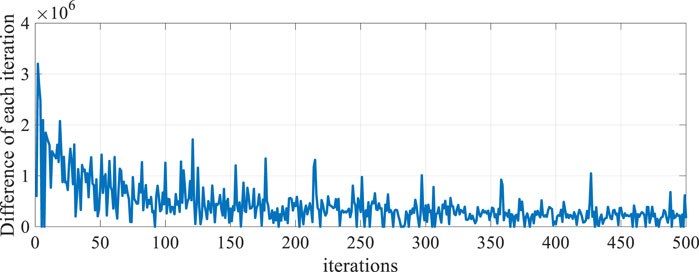
FIGURE 10. Difference of the value function of each iteration.

In this study, the double QL algorithm is applied as the basis for the bi-level energy management rolling optimization process, and the design process of the bi-level EMS will be analyzed in detail later.

4.2 Controller implementation

In this study, the state transfer equation of the MPC controller can be expressed as

$x\left(t+1\right)=f\left(x\left(t\right),u\left(t\right),w\left(t\right)\right),(27)$

where $x\left(t\right)$ denotes the system state variable at time $t$, $u\left(t\right)$ denotes the control variable at time $t$, and $w\left(t\right)$ denotes the random perturbation variable, such as the predicted speed. In the energy management optimization problem of this study, the state variable of the system is the battery, i.e., $x=SOC$; the system control variable is the battery power, i.e., $u=P_{ess}$; and the system stochastic perturbation is the predicted vehicle speed. The prediction time domain $N_p$ of the MPC controller designed in this study is equal to the control time domain $N_c$, both of which are 10 s. The optimized indicator function in each prediction time domain can be expressed as

$J_t=\min {\displaystyle \sum }_t^{t+N_p}{f}_{fuel}\left(t\right)+f_{soc}\left(t\right),(28)$

where $J_t$ is the optimization target in the prediction time domain $\left[t,t+N_p\right]$, $f_{fuel}\left(t\right)$ represents the instantaneous fuel consumption function at each moment, i.e., $f_{fuel}\left(t\right)=Fue{l}_{rate}\left(t\right)$, and $f_{soc}\left(t\right)$ denotes the cost of deviation of the battery $SOC\left(t\right)$ from the reference trajectory $SO{C}_{ref}\left(t\right)$ at time $t$, which is expressed as

$f_{soc}=\left\{\begin{array}{l}0SOC\left(t\right)>SO{C}_{ref}\left(t\right)\\ \alpha {\left(SOC\left(t\right)-SO{C}_{ref}\left(t\right)\right)}^{2}SOC\left(t\right)<SO{C}_{ref}\left(t\right)\end{array}\right.,(29)$

where $\alpha$ denotes a positive weighting factor. The purpose of setting the cost function for the battery's $SOC$ is to ensure that the actual $SOC$ fluctuates around the $SOC$ reference trajectory.

The rolling optimization processes of the designed bi-level energy management controller are narrated as follows.

1) According to the speed and acceleration of future driving conditions, the QL speed predictor is employed to estimate the speed sequence $v_{t+1},v_{t+2},\dots v_{t+N_p}$ in the prediction time domain.

2) The power demand sequence $P_{drive,t+1},P_{drive,t+2},\dots P_{drive,t+N_p}$ in the predicted time domain is calculated from Eqs 3, 4 and the velocity sequence $v_{t+1},v_{t+2},\dots v_{t+N_p}$.

3) The reference SOC trajectory $SO{C}_{ref}\left(t,t+N_p\right)$ is used for rolling optimization in combination with the double QL controller. The rolling optimization process is shown in Table 4. In the rolling optimization process, the two $Q$ matrixes obtained from the double QL controller training are denoted as $Q_{original\_A}$ and $Q_{original\_B}$, and the two Q matrixes involved in the rolling optimization are denoted as $Q_{roll\_A}$ and $Q_{roll\_B}$. The state space and action space in the roll optimization process are consistent with the settings in the double QL controller.

4) After a feedback correction session, the first control variable in the control time domain is output to the PHEV model. It should be noted here that since the double QL controller has converged during the training of the offline controller, the optimization process of the bi-level energy management is performed by rolling the optimization with the predicted time domain only and no more multiple iterations are performed.

TABLE 4

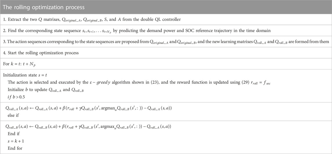
TABLE 4. Rolling optimization process.

The process of MPC rolling optimization is shown in Figure 11. For each step of the rolling optimization, the inputs are the speed prediction sequence, SOC reference value, and demand power sequence in the predicted time domain. The two $Q$ matrixes $Q_{original\_A}$ and $Q_{original\_B}$ are obtained from these three inputs, which are involved in the rolling optimization process, and the two matrixes are employed to perform optimization in the predicted time domain based on Eq. 25.

FIGURE 11

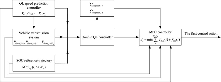
FIGURE 11. Principle of MPC rolling optimization.

5 Results and discussion

In this section, four standard driving conditions are applied as the test data set, i.e., WVUSUB, NEDC, and two real-world driving cycles (KM1 and KM2). These cycles are combined into three different sets, as shown in Figure 12; the first cycle is composed of three WVUSUB and three NEDC, referred to as Cycle 1; the second cycle is composed of five KM1, and the third cycle is composed of 12 KM2. There are two reasons for setting two actual working conditions KM1 and KM2: the first is to verify the effectiveness of the proposed strategy under training conditions of different time lengths, while on the other hand, it is to ensure that different energy management strategies can reduce the SOC to the lowest threshold. The performance of the proposed method is evaluated from the following three perspectives: first, the effectiveness of the proposed method is compared with the double QL offline controller, QL, CD/CS, and SDP. Second, considering that the SOC trajectory of double QL is utilized as the reference trajectory for the design of the proposed method, three different SOC reference trajectories are utilized for expanding the application scope of the proposed method to show the applicability of the proposed method in different SOC reference trajectories. Finally, the computational efficiency of the proposed method is analyzed to verify its practicality.

FIGURE 12

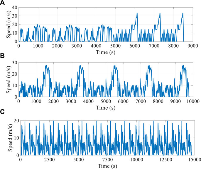
FIGURE 12. Test cycles: (A) Cycle 1; (B) 5 KM1; (C) 12 KM2.

5.1 Comparison with different methods

Table 5 lists the comparison results of fuel consumption for different EMSs under three cycle sets with SOC correction. It can be noted that the fuel-saving effect of the double QL method is better than that of the QL method because the double QL avoids the overestimation of the values caused by a single Q matrix in the QL method. Moreover, since the SOC curve of the double QL method is applied as the reference trajectory, fuel consumption of the proposed method is also closer to the double QL method. Furthermore, when compared to the SDP method, the fuel consumption of the proposed method is 2.73%, 3.38%, and 1.57% higher under the three different driving cycles, respectively, and is approximately closer to that of the SDP method. In addition, the fuel consumption of the proposed method is only 0.32% when compared to that of the QL method under a 12-KM2 driving cycle.

TABLE 5

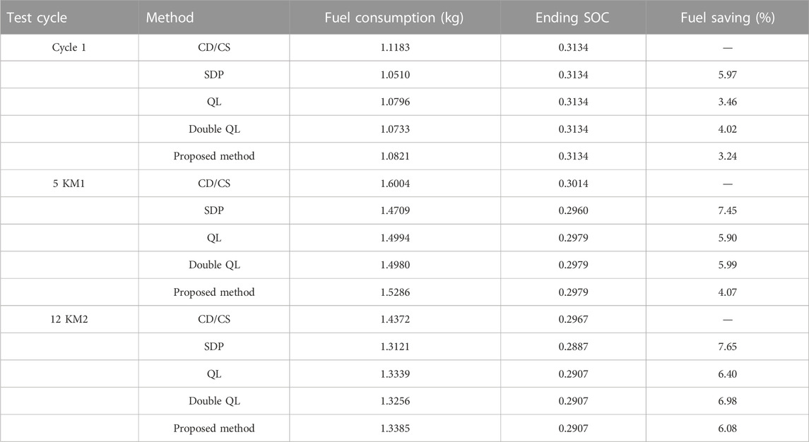
TABLE 5. Comparison of the fuel consumption result of different methods.

The SOC curves of different EMSs are shown in Figure 13. As the penalty function of adding the SOC in the rolling optimization process, it can be noted that the SOC trajectory of the proposed strategy can effectively track the reference trajectory and fluctuate around the reference trajectory. To further verify the effectiveness of the proposed method, Figure 14 depicts the engine efficiency of the SDP, double QL, and the proposed method under different verification cycles, from which it can be seen that these control methods make the engine work in a more efficient region. Moreover, taking 12 KM2 as an example, the engine operating point of the proposed method is the closest one to the SDP method and therefore fuel consumption of the proposed strategy is also the closest method to that of the SDP method. In summary, different methods are utilized to compare fuel consumption, and the comparison results demonstrate that the proposed method features the effectiveness in fuel saving from different perspectives.

FIGURE 13

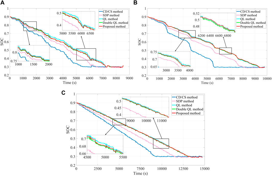
FIGURE 13. SOC curves of different methods: (A) Cycle 1; (B) 5 KM1; and (C) 12 KM2

FIGURE 14

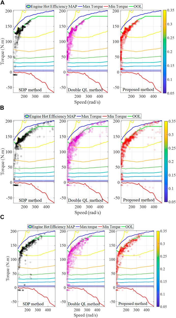
FIGURE 14. Engine efficiency of different methods under different driving cycles: (A) Cycle 1; (B) 5 KM1; and (C) 12 KM2.

5.2 Tracking effect of different reference trajectories

The rolling optimization process and reference trajectory of the proposed method are based on the double QL offline controller. To further validate the learning effect of the proposed method, three different SOC reference trajectories, that include SDP, QL, and liner distance, are employed to validate the extension of the proposed method. Among them, the linear distance reference trajectory is given as

$SO{C}_{dis}\left(t\right)=SO{C}_{init}-\frac{Di{s}_{drive}}{Di{s}_{all}}\left(SO{C}_{init}-SO{C}_{low}\right),(30)$

where $SO{C}_{dis}\left(t\right)$ denotes the linear distance for the reference SOC at time step $t$. $SO{C}_{init}$ indicates the initial SOC value, which is set as 0.9. $SO{C}_{low}$ means the final SOC value at the end of the driving cycle, which is set as 0.3. $Di{s}_{all}$ represents the distance of the entire driving cycle. $Di{s}_{drive}$ stands for the distance that has been traveled.

Figure 15 shows the SOC curves of the proposed method for these three different SOC trajectories under 5 KM1 and 12 KM2 driving cycles. It can be noted that the SOC curves obtained by the proposed method are consistent with the decreasing trend under different working cycles, and all of them can be well tracked. Similarly, according to the enlarged figure of Figure 13, it can also be seen that the SOC curve of the proposed method basically floats above and below the reference trajectory due to the setting of the penalty function for the SOC during the rolling optimization. From this point of view, the proposed method can track the reference trajectory effectively.

FIGURE 15

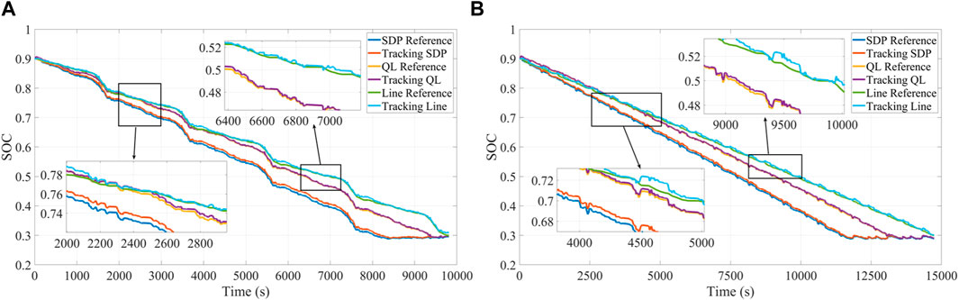
FIGURE 15. SOC curves under different reference trajectories: (A) 5 KM1. (B) 12 KM2.

Table 6 shows the fuel consumption results of the proposed method under three different reference trajectories. Taking the CD/CS fuel consumption as the benchmark, the proposed method yields high fuel economy for all three different reference trajectories. In the 5-KM1 driving cycle, fuel saving of the proposed method under the three reference tracks are 5.58%, 4.22%, and 3.89%, respectively. In the 12-KM2 driving cycle, fuel saving of the proposed method under the three reference tracks are 6.64%, 5.06%, 4.33%, respectively. Comparing the fuel consumption of the three different reference trajectories, it can be observed that the SDP reference trajectory shows the best fuel saving performance, and the worst is the linear distance reference trajectory. The reason for this phenomenon can be attributed to the SDP strategy, which is a global suboptimal method, while the QL is a local optimal method, therefore the reference trajectories obtained by these two methods possess the global suboptimal or local optimal characteristics, while the linear distance reference trajectory does not feature the optimization characteristics, and the fuel economy is the lowest among these trajectories.

TABLE 6

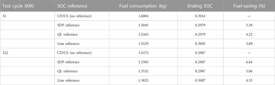
TABLE 6. Fuel consumption results under three different reference trajectories.

5.3 Computational efficiency analysis

In this study, the calculation time for a single step of the proposed method is evaluated on a laptop computer, which is equipped with the Intel Core i7 @2.3 GHz processor and 16 GB RAM. Note that the computational time does not include the training time for the speed predictor and double QL offline controller but only includes the time for speed prediction and computation time for the MPC controller. The calculation time is tabulated in Table 7, and it can be noted that the calculation time of each step ranges from 8.36 to 10.07 ms, which indicates that the proposed method has the potential for online implementation.

TABLE 7

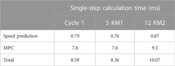
TABLE 7. Computational efficiency.

6 Conclusion

This study proposes a bi-level EMS to solve the energy management problem of PHEVs. First, considering the uncertainty of acceleration in the process of driving, the acceleration is taken as the action, and a QL-based speed predictor is constructed by the reinforcement learning algorithm. Second, considering different speed intervals during vehicle driving, the double QL method is utilized to establish an offline controller and its fuel economy is verified. Then, the QL speed predictor and double QL offline controller are integrated into the MPC, in which the double QL method performs the rolling optimization to construct a bi-level energy management controller. The effectiveness, applicability, and practicality of the proposed method are verified by standard and measured driving cycles. The results show that the proposed method is capable of exerting high fuel economy control for the PHEVs with favorable tracking performance for the different reference trajectories, and the calculation efficiency of the proposed method shows the potential capacity for real-time applications.

Our future work will focus on considering the impact of traffic information on vehicle fuel economy and the study of fuel economy of intelligently connected vehicles with intelligent traffic information. In addition, the proposed method should be further optimized by hardware-in-the-loop and real vehicle experiments.

Data availability statement

The original contributions presented in the study are included in the article/Supplementary Material; further inquiries can be directed to the corresponding author.

Author contributions

XY: supervision, investigation, discussion, and writing. CJ: methodology. MZ: methodology. HH: writing, discussion, and editing.

Conflict of interest

The authors declare that the research was conducted in the absence of any commercial or financial relationships that could be construed as a potential conflict of interest.

Publisher’s note

All claims expressed in this article are solely those of the authors and do not necessarily represent those of their affiliated organizations, or those of the publisher, editors, and reviewers. Any product that may be evaluated in this article, or claim that may be made by its manufacturer, is not guaranteed or endorsed by the publisher.

References

Biswas, A., and Emadi, A. (2019). Energy management systems for electrified powertrains: State-of-the-Art review and future trends. IEEE Trans. Veh. Technol. 68 (7), 6453–6467. doi:10.1109/tvt.2019.2914457

CrossRef Full Text | Google Scholar

Chen, Z., Gu, H., Shen, S., and Shen, J. (2022). Energy management strategy for power-split plug-in hybrid electric vehicle based on MPC and double Q-learning. Energy 245, 123182. doi:10.1016/j.energy.2022.123182

CrossRef Full Text | Google Scholar

Chen, Z., Hu, H., Wu, Y., Xiao, R., Shen, J., and Liu, Y. (2018). Energy management for a power-split plug-in hybrid electric vehicle based on reinforcement learning. Appl. Sciences-Basel 8 (12), 2494. doi:10.3390/app8122494

CrossRef Full Text | Google Scholar

Chen, Z., Hu, H., Wu, Y., Zhang, Y., Li, G., and Liu, Y. (2020). Stochastic model predictive control for energy management of power-split plug-in hybrid electric vehicles based on reinforcement learning. Energy 211, 118931. doi:10.1016/j.energy.2020.118931

CrossRef Full Text | Google Scholar

Chen, Z., Liu, Y., Zhang, Y., Lei, Z., Chen, Z., and Li, G. (2022). A neural network-based ECMS for optimized energy management of plug-in hybrid electric vehicles. Energy 243, 122727. doi:10.1016/j.energy.2021.122727

CrossRef Full Text | Google Scholar

Chen, Z., Mi, C. C., Xia, B., and You, C. (2014). Energy management of power-split plug-in hybrid electric vehicles based on simulated annealing and Pontryagin's minimum principle. J. Power Sources 272, 160–168. doi:10.1016/j.jpowsour.2014.08.057

CrossRef Full Text | Google Scholar

Chen, Z., Xia, B., You, C., and Mi, C. C. (2015). A novel energy management method for series plug-in hybrid electric vehicles. Appl. Energy 145, 172–179. doi:10.1016/j.apenergy.2015.02.004

CrossRef Full Text | Google Scholar

Cheng, S., Chen, X., Fang, S. n., Wang, X. y., Wu, X. h., et al. (2020). Longitudinal autonomous driving based on game theory for intelligent hybrid electric vehicles with connectivity. Appl. Energy 268, 115030. doi:10.1016/j.apenergy.2020.115030

CrossRef Full Text | Google Scholar

Ganesh, A. H., and Xu, B. (2022). A review of reinforcement learning based energy management systems for electrified powertrains: Progress, challenge, and potential solution. Renew. Sustain. Energy Rev. 154, 111833. doi:10.1016/j.rser.2021.111833

CrossRef Full Text | Google Scholar

Guo, J., He, H., Peng, J., and Zhou, N. (2019). A novel MPC-based adaptive energy management strategy in plug-in hybrid electric vehicles. Energy 175, 378–392. doi:10.1016/j.energy.2019.03.083

CrossRef Full Text | Google Scholar

Guo, N., Zhang, X., Yuan, Z., Guo, L., and Du, G. (2021). Real-time predictive energy management of plug-in hybrid electric vehicles for coordination of fuel economy and battery degradation. Energy 214, 119070. doi:10.1016/j.energy.2020.119070

CrossRef Full Text | Google Scholar

Guo, N., Zhang, X., Zou, Y., Du, G., Wang, C., and Guo, L. (2021). Predictive energy management of plug-in hybrid electric vehicles by real-time optimization and data-driven calibration. IEEE Trans. Veh. Technol. 71, 5677–5691. doi:10.1109/tvt.2021.3138440

CrossRef Full Text | Google Scholar

Guo, N., Zhang, X., and Zou, Y. (2022). Real-time predictive control of path following to stabilize autonomous electric vehicles under extreme drive conditions. Automot. Innov. 5, 453–470. doi:10.1007/s42154-022-00202-3

CrossRef Full Text | Google Scholar

Han, L., Jiao, X., and Zhang, Z. (2020). Recurrent neural network-based adaptive energy management control strategy of plug-in hybrid electric vehicles considering battery aging. Energies 13 (1), 202. doi:10.3390/en13010202

CrossRef Full Text | Google Scholar

Hasselt, H. V., Guez, A., and Silver, D. J. C. (2015). “Deep reinforcement learning with double Q-learning,”. arXiv:1509.06461.

Google Scholar

He, H., Wang, Y., Han, R., Han, M., Bai, Y., and Liu, Q. (2021). An improved MPC-based energy management strategy for hybrid vehicles using V2V and V2I communications. Energy 225, 120273. doi:10.1016/j.energy.2021.120273

CrossRef Full Text | Google Scholar

Jeong, J., Lee, D., Kim, N., Zheng, C., Park, Y.-I., and Cha, S. W. (2014). Development of PMP-based power management strategy for a parallel hybrid electric bus. Int. J. Precis. Eng. Manuf. 15 (2), 345–353. doi:10.1007/s12541-014-0344-7

CrossRef Full Text | Google Scholar

Lei, Z., Qin, D., Zhao, P., Li, J., Liu, Y., and Chen, Z. (2020). A real-time blended energy management strategy of plug-in hybrid electric vehicles considering driving conditions. J. Clean. Prod. 252, 119735. doi:10.1016/j.jclepro.2019.119735

CrossRef Full Text | Google Scholar

Li, S. E., Guo, Q., Xin, L., Cheng, B., and Li, K. (2017). Fuel-saving servo-loop control for an adaptive cruise control system of road vehicles with step-gear transmission. IEEE Trans. Veh. Technol. 66 (3), 2033–2043. doi:10.1109/tvt.2016.2574740

CrossRef Full Text | Google Scholar

Lin, X., Wu, J., and Wei, Y. (2021). An ensemble learning velocity prediction-based energy management strategy for a plug-in hybrid electric vehicle considering driving pattern adaptive reference SOC. Energy 234, 121308. doi:10.1016/j.energy.2021.121308

CrossRef Full Text | Google Scholar

Liu, Y., Li, J., Gao, J., Lei, Z., Zhang, Y., and Chen, Z. (2021). Prediction of vehicle driving conditions with incorporation of stochastic forecasting and machine learning and a case study in energy management of plug-in hybrid electric vehicles. Mech. Syst. Signal Process. 158, 107765. doi:10.1016/j.ymssp.2021.107765

CrossRef Full Text | Google Scholar

Overington, S., and Rajakaruna, S. (2015). High-efficiency control of internal combustion engines in blended charge depletion/charge sustenance strategies for plug-in hybrid electric vehicles. IEEE Trans. Veh. Technol. 64 (1), 48–61. doi:10.1109/tvt.2014.2321454

CrossRef Full Text | Google Scholar

Peng, J., He, H., and Xiong, R. (2017). Rule based energy management strategy for a series-parallel plug-in hybrid electric bus optimized by dynamic programming. Appl. Energy 185, 1633–1643. doi:10.1016/j.apenergy.2015.12.031

CrossRef Full Text | Google Scholar

Quan, S., Wang, Y.-X., Xiao, X., He, H., and Sun, F. (2021). Real-time energy management for fuel cell electric vehicle using speed prediction-based model predictive control considering performance degradation. Appl. Energy 304, 117845. doi:10.1016/j.apenergy.2021.117845

CrossRef Full Text | Google Scholar

Ruan, S., Ma, Y., Yang, N., Xiang, C., and Li, X. (2022). Real-time energy-saving control for HEVs in car-following scenario with a double explicit MPC approach. Energy 247, 123265. doi:10.1016/j.energy.2022.123265

CrossRef Full Text | Google Scholar

Singh, K. V., Bansal, H. O., and Singh, D. (2021). Fuzzy logic and Elman neural network tuned energy management strategies for a power-split HEVs. Energy 225, 120152. doi:10.1016/j.energy.2021.120152

CrossRef Full Text | Google Scholar

Sun, X., Zhou, Y., Huang, L., and Lian, J. (2021). A real-time PMP energy management strategy for fuel cell hybrid buses based on driving segment feature recognition. Int. J. Hydrogen Energy 46 (80), 39983–40000. doi:10.1016/j.ijhydene.2021.09.204

CrossRef Full Text | Google Scholar

Tang, X., Chen, J., Pu, H., Liu, T., and Khajepour, A. (2022). Double deep reinforcement learning-based energy management for a parallel hybrid electric vehicle with engine start–stop strategy. IEEE Trans. Transp. Electrification 8 (1), 1376–1388. doi:10.1109/tte.2021.3101470

CrossRef Full Text | Google Scholar

Watkins, C., Christopher, J., and Dayan, P. J. M. L. (1992). Technical note: Q-learning. Mach. Learn. 8, 279–292. doi:10.1023/a:1022676722315

CrossRef Full Text | Google Scholar

Wu, Y., Zhang, Y., Li, G., Shen, J., Chen, Z., and Liu, Y. (2020). A predictive energy management strategy for multi-mode plug-in hybrid electric vehicles based on multi neural networks. Energy 208, 118366. doi:10.1016/j.energy.2020.118366

CrossRef Full Text | Google Scholar

Yang, N., Han, L., Xiang, C., Liu, H., and Li, X. (2021). An indirect reinforcement learning based real-time energy management strategy via high-order Markov chain model for a hybrid electric vehicle. Energy 236, 121337. doi:10.1016/j.energy.2021.121337

CrossRef Full Text | Google Scholar

Zhang, L., Liu, W., and Qi, B. (2020). Energy optimization of multi-mode coupling drive plug-in hybrid electric vehicles based on speed prediction. Energy 206, 118126. doi:10.1016/j.energy.2020.118126

CrossRef Full Text | Google Scholar

Zhang, W., Wang, J., Liu, Y., Gao, G., Liang, S., and Ma, H. (2020). Reinforcement learning-based intelligent energy management architecture for hybrid construction machinery. Appl. Energy 275, 115401. doi:10.1016/j.apenergy.2020.115401

CrossRef Full Text | Google Scholar

Zhang, Y., Chu, L., Fu, Z., Xu, N., Guo, C., Zhao, D., et al. (2020). Energy management strategy for plug-in hybrid electric vehicle integrated with vehicle-environment cooperation control. Energy 197, 117192. doi:10.1016/j.energy.2020.117192

CrossRef Full Text | Google Scholar

Zhou, Y., Li, H., Ravey, A., and Pera, M.-C. (2020). An integrated predictive energy management for light-duty range-extended plug-in fuel cell electric vehicle. J. Power Sources 451, 227780. doi:10.1016/j.jpowsour.2020.227780

CrossRef Full Text | Google Scholar

Zhou, Y., Ravey, A., and Pera, M.-C. (2020). Multi-objective energy management for fuel cell electric vehicles using online-learning enhanced Markov speed predictor. Energy Convers. Manag. 213, 112821. doi:10.1016/j.enconman.2020.112821

CrossRef Full Text | Google Scholar

Nomenclature

PHEV plug-in hybrid electric vehicle

EMS energy management strategy

CD/CS charge depleting/charge sustaining

SOC state of charge

DP dynamic programming

PMP Pontryagin’s minimum principle

GT game theory

ECMS equivalent consumption minimization strategy

MPC model predictive control

RL reinforcement learning

BP back propagation

QL Q-learning

SDP stochastic DP

OOL engine optimal operating line

RMSE root-mean-square error

$\mathit{F}\mathit{u}\mathit{e}{\mathit{l}}_{\mathit{t}\mathit{o}\mathit{t}\mathit{a}\mathit{l}}$ total fuel consumption

$\mathit{F}\mathit{u}\mathit{e}{\mathit{l}}_{\mathit{r}\mathit{a}\mathit{t}\mathit{e}}$ instantaneous fuel consumption

$\mathit{T}$ total time of the whole driving cycle

${\mathit{\omega }}_{\mathit{e}\mathit{n}\mathit{g}}$ engine speed

${\mathit{T}}_{\mathit{e}\mathit{n}\mathit{g}}$ engine torque

${\mathit{P}}_{\mathit{d}\mathit{r}\mathit{i}\mathit{v}\mathit{e}}$ power demand of the vehicle

${\mathit{F}}_{\mathit{f}}$ rolling resistance

${\mathit{F}}_{\mathit{i}}$ grade resistance

${\mathit{F}}_{\mathit{w}}$ air resistance

${\mathit{F}}_{\mathit{j}}$ acceleration resistance

$\mathit{v}$ vehicle speed

$\mathit{m}$ vehicle mass

$\mathit{g}$ gravitational acceleration

$\mathit{f}$ rolling resistance coefficient

$\mathit{\alpha }$ slope of travel

${\mathit{C}}_{\mathit{d}}$ air resistance coefficient,

$A_{wind}$

windward area of the vehicle

$\mathit{\delta }$ mass conversion factor of the vehicle

${\mathit{P}}_{\mathit{f}\mathit{i}\mathit{n}\mathit{a}\mathit{l}}$ power of the main gearbox

${\mathit{P}}_{\mathit{e}\mathit{n}\mathit{g}}$ power of the engine

${\mathit{P}}_{\mathit{e}\mathit{s}\mathit{s}}$ power of the battery

${\mathit{P}}_{\mathit{m}\mathit{o}\mathit{t}\mathbf{1}}$ power of motor 1

${\mathit{P}}_{\mathit{m}\mathit{o}\mathit{t}\mathbf{2}}$ power of motor 2

${\mathit{P}}_{\mathit{e}\mathit{l}\mathit{e}\mathit{c}}$ power of the electrical accessories

${\mathit{\eta }}_{\mathit{f}\mathit{i}\mathit{n}\mathit{a}\mathit{l}}$ transmission efficiency of the main reducer

${\mathit{\eta }}_{\mathit{g}\mathit{e}\mathit{a}\mathit{r}}$ transmission efficiency of the transmission unit

${\mathit{\eta }}_{\mathit{m}\mathit{o}\mathit{t}\mathbf{1}}$ transmission efficiency of motor 1

${\mathit{\eta }}_{\mathit{m}\mathit{o}\mathit{t}\mathbf{2}}$ transmission efficiency of motor 2

${\mathit{\omega }}_{\mathit{m}\mathit{o}\mathit{t}\mathbf{1}}$ speed of motor 1

${\mathit{\omega }}_{\mathit{m}\mathit{o}\mathit{t}\mathbf{2}}$ speed of motor 2

${\mathit{T}}_{\mathit{m}\mathit{o}\mathit{t}\mathbf{1}}$ torque of motor 1

${\mathit{T}}_{\mathit{m}\mathit{o}\mathit{t}\mathbf{2}}$ torque of motor 2

$\mathit{\mu }$ gear ratio of the planetary gear

${\mathit{I}}_{\mathit{e}\mathit{s}\mathit{s}}$ battery current

$\mathit{O}\mathit{C}\mathit{V}$ open-circuit voltage

${\mathit{R}}_{\mathbf{int}}$ internal resistance

$\mathit{S}\mathit{O}\mathit{C}\left(\mathit{t}\right)$ $SOC$ value at time step t

$\mathit{S}\mathit{O}{\mathit{C}}_{\mathit{i}\mathit{n}\mathit{i}\mathit{t}}$ initial $SOC$ value

${\mathit{C}}_{\mathit{e}\mathit{s}\mathit{s}}$ battery capacity

$\mathit{S}$ state variable in QL

$\mathit{A}$ action variable in QL

$\mathit{R}$ reward function in QL

${\mathit{a}}^{\prime }$ action corresponding to the next state

$\mathit{\beta }$ learning efficiency

${\mathit{v}}_{\mathit{s}\mathit{p}\mathit{d}}$ current speed state

${\mathit{v}}_{\mathit{p}\mathit{r}\mathit{e}}\left(\mathit{t}\right)$ predicted velocity

${\mathit{v}}_{\mathit{r}\mathit{e}\mathit{a}\mathit{l}}\left(\mathit{t}\right)$ real velocity

${\mathit{v}}_{\mathit{d}\mathit{i}\mathit{f}\mathit{f}}\left(\mathit{t}\right)$ difference between the predicted vehicle speed and actual value

$\mathit{E}\mathit{r}\mathit{r}\left(\mathit{t}\right)$ RMSE value of the predicted velocity series and actual velocity series

${\mathit{t}}_{\mathit{p}}$ predicted time domain

${\mathit{v}}_{\mathit{t},\mathit{i}}^{\mathit{p}\mathit{r}\mathit{e}}$ predicted speed at the $i‑th$ second after time $t$

${\mathit{v}}_{\mathit{t},\mathit{i}}^{\mathit{r}\mathit{e}\mathit{a}\mathit{l}}$ actual velocity at the $i‑th$ second after time $t$

$\mathit{e}\mathit{n}\mathit{g}\_\mathit{o}\mathit{n}=\mathbf{1}$ engine is turned on

$\mathit{e}\mathit{n}\mathit{g}\_\mathit{o}\mathit{n}=\mathbf{0}$ engine is turned off

$\mathit{F}\mathit{u}\mathit{e}{\mathit{l}}_{\mathit{r}\mathit{a}\mathit{t}\mathit{e}\_\mathbf{m}\mathbf{a}\mathbf{x}}$ the maximum value of engine fuel consumption MAP

${\mathit{P}}_{\mathit{e}\mathit{n}\mathit{g}\_\mathit{o}\mathit{n}}$ threshold value for engine turned on

$\mathit{c}$ a random number from 0 to 1

$\mathit{\epsilon }$ greed factor

$\mathit{x}\left(\mathit{t}\right)$ system state variable at time $t$

$\mathit{u}\left(\mathit{t}\right)$ control variable at time $t$

$\mathit{w}\left(\mathit{t}\right)$ random perturbation variable

${\mathit{N}}_{\mathit{p}}$ prediction time domain

${\mathit{N}}_{\mathit{c}}$ control time domain

${\mathit{J}}_{\mathit{t}}$ optimization target in the prediction time domain $\left[t,t+N_p\right]$

$\mathit{S}\mathit{O}{\mathit{C}}_{\mathit{r}\mathit{e}\mathit{f}}\left(\mathit{t}\right)$ SOC reference trajectory

${\mathit{f}}_{\mathit{f}\mathit{u}\mathit{e}\mathit{l}}\left(\mathit{t}\right)$ instantaneous fuel consumption function at each moment

${\mathit{f}}_{\mathit{s}\mathit{o}\mathit{c}}\left(\mathit{t}\right)$ cost of deviation of the battery’s SOC from the reference trajectory at time $t$

$\mathit{\alpha }$ a positive weighting factor

$\mathit{S}\mathit{O}{\mathit{C}}_{\mathit{d}\mathit{i}\mathit{s}}\left(\mathit{t}\right)$ linear distance for the reference SOC at time step $t$

$\mathit{S}\mathit{O}{\mathit{C}}_{\mathit{l}\mathit{o}\mathit{w}}$ final SOC value at the end of the driving cycle