A trading optimization model for virtual power plants in day-ahead power market considering uncertainties

Background: The day-ahead power market is an important part of the spot market. In the day-ahead market, participants make short-term forecasts of the load and output to propose the bidding curve more precisely. As energy aggregators that have regulatory resources, virtual power plants (VPPs) need to consider the uncertainty of distributed renewable energy output when participating in power market transactions.

Methods: This paper analyzes the uncertainty and built an optimization model for VPP in day-ahead power market considering the uncertainty from both inner parts and the market environment. To verify the model, a simulation study is ran.

Results: And the study results show the following: 1) the forecasting model is more efficient than the traditional algorithm in terms of accuracy, and 2) the confidence levels are not fully positive with the benefit of VPPs.

Discussion: Improving the confidence level could reduce the uncertainty brought by renewable energy, but could also cause conservative trading behavior and affect the consumption of renewable energy.

1 Introduction

In response to the call for low-carbon development, clean energy has gradually become the focus of energy transformation. As control carriers for aggregating distributed energy and energy storage, virtual power plants (VPPs) can improve energy utilization efficiency and reduce clean energy curtailment through flexible regulation (Tan and Yang, 2019). In market transactions, VPPs can further allot power resources in another way. Considering the fluctuating generation of renewable energy, the uncertainty of power sources should be overcome at the outset (Zhou et al., 2017).

The uncertainty and volatility of renewable energy output will cause deviations in the spot market, leading to power curtailment or load loss. Many researches have been made to solve the uncertainty of renewable energy output. Multiple correction of bidding power in the day-ahead market based on the Spanish power market mechanism was proposed, realizing an accurate match between generation bidding and real-time load (JafariZareipourSchellenberg and Amjady, 2014). It was noted that the uncertainty of renewable energy output is key to realizing stable operation of the spot market (Meibom et al., 2011). A mixed-integer programming scheduling model of VPP was proposed considering wind power output, electric vehicles (EVs), and electricity price fluctuations in the day-ahead market by using the point estimation method (Shayegan-Rad et al., 2017). The randomness and fluctuation of wind power and photovoltaic (PV) output using the kernel density estimation method were considered (Bai et al., 2018), generating a large number of wind and PV processing scenes and forming an economic power system dispatching model with improved forecasting. The output of a wind turbine in combination with stochastic programming theory was simulated (HeydarianForushani et al., 2014), realizing effective control of the uncertainty of wind power in market transactions. Due to the uncertainty of distributed wind power and PV power generation, it is necessary to consider methods to overcome the uncertainty in transaction optimization. Commonly used methods include scenario reduction (Wu et al., 2019; Sun et al., 2021) and intelligent algorithm prediction n (Kong et al., 2015; Shu et al., 2020). Using the Monte Carlo method, literature (Dong et al., 2018) forecasted the EV load considering demand response (DR) management. Using the random forest method, literature (Niu et al., 2020) improved the intelligent algorithm and selected typical climate days as examples for analysis. An optimal bidding model based on short-term probability forecasting for wind power was constructed in (Pinson et al., 2007).

In addition, market participants often consider the balance between risk and profit when conducting market transactions. Therefore, the CVaR method is introduced to measure the relevant returns under a set credit level. Based on the load aggregator and using the CVaR method, literature (Zhang et al., 2020) proposed bidding decisions in power market transactions. Based on data of the PJM power market and the risk of price fluctuation, literature (Liu et al., 2020) used the CVaR method to measure the risk. Using CVaR risk measurement, aiming at minimizing the loss of power purchasers and considering the factors of peak–valley time of use (TOU) and price, an optimal combination was proposed in (Zhu and Xie, 2015).

In the day-ahead power market, it is also necessary to consider price uncertainty and load change trend in the market in combination with the market mechanism. The literature (Jadfari et al., 2014) analyzed the intraday market mechanism and put forward an intraday trading mechanism of wind power dynamic output correction. In literature (Riveraion et al., 2015), the maximum expected return of VPP market transactions is taken as the objective function, constructed a short-term VPP power transaction optimization model, and used the scenario simulation method to reflect price uncertainty in the day-ahead market. Literature (Zamani et al., 2016) used the optimal allocation and market price factors in VPP and proposed an optimal day-ahead scheduling model of VPP electric and thermal energy. Literature (Fan et al., 2015; Duan et al., 2016) constrained the uncertainty of wind and PV output in VPP and constructed an optimal two-level scheduling model.

Among the previous research, few studies focused on decision-making for VPPs in the day-ahead market considering uncertainty from both inner VPP and market trading sides. In this paper, the uncertainty of VPPs participating in market trading is divided into two aspects, intrinsic and extrinsic factors, including the generation uncertainty of wind power and PV, and the risk preference of decision-makers. Then, a combined forecasting method, the EEMD-CS-ELM forecasting model, is proposed to reduce the generation uncertainty of wind power and PV units. And CVaR theory is introduced to analyze the external uncertainty of VPPs in market trading environment. Finally, a case study is examined to verify both the rationality of the EEMD-CS-ELM model and the application of CVaR theory in this situation.

2 Uncertainty of virtual power plant under day-ahead transaction

2.1 Uncertainty modeling of virtual power plants

2.1.1 Uncertainty of wind power and photovoltaic output

In the context of market-oriented reform, distributed wind power and PV generally cannot participate in market transactions directly due to their small capacity. VPP can participate in market transactions through the aggregation of distributed energy. With its own flexible regulation ability and the introduction of energy storage and other components, the utilization efficiency of distributed energy can be improved. In addition, the incoming wind power is affected by geographical location and time period, and photovoltaic is affected by the time-period distribution of weather and radiation intensity. Their generation curves have strong volatility and randomness. Therefore, in day-ahead market transactions, the internal uncertainty from wind and PV output should be considered at the outset.

2.1.2 Modeling of uncertain output of wind power plant

The output uncertainty of a wind power plant (WPP) depends on the random characteristics of wind speed, which can usually be described by the Weibull distribution (Zhang et al., 2015). The wind speed calculation model is as follows:

$f\left(v\right)=\left(\frac{k}{c}\right)\cdot {\left(\frac{v}{c}\right)}^{k-1}\cdot e^{-{\left(\frac{v}{c}\right)}^k}(1)$

where v is the wind speed, c is the scale parameter of the Weibull distribution, and k is the state parameter. Based on Eq. 1, the relationship between the real-time output of a wind turbine and the real-time wind speed can be expressed as follows:

$P_t^{WT}=\left\{\begin{array}{cc}0& v<V_{in},v>V_{out}\\ 0.5C_p\rho A_w{v}^3& V_{in}<v<V_{rated}\\ P_{rated}^{WT}& V_{rated}<v<V_{out}\end{array}\right.(2)$

where $P_t^{WT}$ is the output of the wind turbine at time $t$, $C_p$ is the wind power utilization parameter, $\rho$ is the air density, $A_w$ is the vertical projected area of the wind on the swept area of the blade, $P_{rated}^{WT}$ is the rated output of the WPP, and $V_{in}$, $V_{rated}$, and $V_{out}$ are the cut-in, rated, and cut-out wind speed, respectively.

2.1.3 Modeling of uncertain output of PV

The uncertainty of PV comes from the stochastic characteristics of solar radiation intensity, which is usually described by beta distribution (JuTanYuan et al., 2016). The solar radiation intensity model is as follows:

$f_{PV}\left(t\right)=\frac{\mathrm{\Gamma }\left(\alpha +\beta \right)}{\mathrm{\Gamma }\left(\alpha \right)+\mathrm{\Gamma }\left(\beta \right)}{\left(\frac{r}{r_{\max }}\right)}^{\alpha -1}{\left(1-\frac{r}{r_{\max }}\right)}^{\beta -1}(3)$

where $r$ is the solar irradiance, $r_{\max }$ is the maximum radiation, and $\alpha$ and $\beta$ are the shape parameters of beta distribution, which will lead to changes in the shape of its probability density curve. $\alpha$ and $\beta$ can be calculated by expectation $\mu$ and variance $\delta$:

$\alpha =\mu \left[\frac{\mu \left(1-\mu \right)}{{\delta }^2}-1\right](4)$

$\beta =\left(1-\mu \right)\left[\frac{\mu \left(1-\mu \right)}{{\delta }^2}-1\right](5)$

Based on the calculation of solar radiation intensity, the PV output model is obtained:

$P_t^{PV}={\chi }^{PV}{\rho }^{PV}{\theta }_t(6)$

where ${\chi }^{PV}$ is the transmission efficiency, ${\rho }^{PV}$ is the total area of PV devices, and ${\theta }_t$ is the radiation intensity at time $t$.

2.2 Comprehensive uncertainty analysis of day-ahead market with CVaR

In actual operation, there is a deviation between the actual generation curve of the market entity and the forecasted generation curve reported by the entity. When a VPP participates in market transactions, to improve the consumption amount of distributed wind and PV power, thermal units and energy storage devices will assume the function of flexible standby regulation, which shows that the deviation is mainly caused by wind and PV output. This can be described by introducing the conditional value at risk (CVaR) method, and the basic VaR can be expressed as follows:

$P\left(X<VaR\right)=a(7)$

where $P$ is the possibility that the loss value is less than the VaR, $X$ is the loss value of the assets, and $a$ is the confidence interval.

The confidence level of the basic VaR method does not obey the regular distribution, and changes in the confidence level will have a great impact on the VaR. Therefore, CVaR is introduced to increase conditionality based on the principle of VaR to reflect the additional risk distribution (Li et al., 2021):

$CVaR=E\left(X|X\ge CVaR\right)(8)$

$CVa{R}_a\left(X\right)=E\left[X\left|Va{R}_a\right.\left(X\right)\right]=\frac{1}{1-a}{\int }_{-\infty }^{VaR}xf\left(x\right)dx(9)$

where $Va{R}_a\left(X\right)$ is the VaR when the confidence level is $a$ and $CVa{R}_a\left(X\right)$ is the expectation value when the loss is over $Va{R}_{1-a}\left(X\right)$, $VaR$ is the $a$ quantile of X, and $f\left(x\right)$ is the probability distribution, which is not defined as an absolute continuous function. Considering that the probability density function of the actual output of wind power and PV obeys normal distribution, we performed further analysis of a VPP participating in the day-ahead power market based on generation uncertainty.

3 Optimization model of VPP in day-ahead market based on EEMD-CS-ELM and CVaR

3.1 Processing internal uncertainty of VPPs

3.1.1 Methods

3.1.1.1 Ensemble empirical mode decomposition (EEMD)

Ensemble empirical mode decomposition is a new self-adaptive sequence analysis technique that is based on and overcomes the mode mixing problem of traditional empirical mode decomposition (EMD). EEDM adds a series of Gaussian white noise signals to the original power signal. Combining the statistical features of spectrum equalization distribution, EEMD filters the trends with different features in the original sequence and forms intrinsic modal function (IMF) clustering with features. Finally, the mode mixing problem of EMD is solved by counteracting the Gaussian white noise in each function but retaining the original characteristics of the power sequence. The implementation of EEDM is as follows:

(1) Add Gaussian white noise signals $\kappa \left(t\right)$ to the power signal $P\left(t\right)$ to get a new power signal $P^{\prime }\left(t\right)$:

$P^{\prime }\left(t\right)=P\left(t\right)+\kappa \left(t\right)(10)$

(2) Using the EMD method, calculate $P^{\prime }\left(t\right)$ as

$P^{\prime }\left(t\right)=r_n\left(t\right)+{\displaystyle \sum _{i=1}^n}{I}_i\left(t\right)(11)$

In the formula, $r_n\left(t\right)$ refers to the remnant after decomposition and $I_i\left(t\right)$ refers to the IMF of layer $i$ ($i=\mathrm{1,2},...,n$), which is arranged from high to low in order of frequency.

(3) Add Gaussian white noise signals $j$ times to $P\left(t\right)$, and repeat the above steps to obtain

${P_j}^{\prime }\left(t\right)=P\left(t\right)+{\kappa }_j\left(t\right)=r_{j,n}\left(t\right)+{\displaystyle \sum _{i=1}^n}{I}_{ji}\left(t\right)(12)$

In the formula, $I_{ji}\left(t\right)$ refers to the IMF weight of layer $i$ after adding Gaussian white noise signals $j$ times.

(4) Combined with the statistical mean of the uncorrelated random sequences of an EMD of 0, the whole is averaged to counteract the effect of multiple additive white Gaussian noise on the power signal, and the IMF can be expressed as follows.

$I_i\left(t\right)=\frac{1}{N}{\displaystyle \sum _{j=1}^N}{I}_{ji}\left(t\right)(13)$

During the processing of EEMD, the Gaussian white noise signal should satisfy the condition ${\epsilon }_n=\frac{\epsilon }{\sqrt{N}}$, where $\epsilon$ refers to the amplitude of the Gaussian white noise signal and N refers to the overall average times the signal is added, and when N in the range of 100–300, the signal standard deviation is 0.001–0.5 times; and ${\epsilon }_n$ refers to the error value of the original power signal and the power signal after EEMD processing.

3.1.1.2 Cuckoo search

Cuckoo search (CS) is a kind of nature-inspired heuristic algorithm that was developed in 2009 by XinShe Yang and Suash Deb at Cambridge University. CS is based on the parasitic brooding behavior of cuckoos. The cuckoo lays its eggs in the nest of a host and removes the host’s eggs. Some cuckoo eggs that look like the host’s eggs will have the opportunity to be nurtured. In other cases, the eggs may be recognized and thrown away by the host bird, or the host leaves the nest to look for somewhere else to build a new nest. Then all of the eggs are abandoned. Each egg in the nest represents a solution, and each cuckoo egg represents a new solution. CS replaces the less-than-good solutions in nesting with new and possibly better solutions.

CS works as follows: The cuckoo lays one egg each time in a random nest. The nest in which the egg (solution) with the highest quality is placed will continue to the next-generation. The number of nests in which the cuckoo will put its eggs is fixed, and the probability that the host bird will pick out the cuckoo’s egg is $p_a\in \left[\mathrm{0,1}\right]$.

If the host bird discovers the cuckoo’s egg, it may throw out the egg or find another place to build a nest. If the egg is not discovered, it will successfully hatch and find a new location by Lévy flight. Considering the features of Lévy flight in the process of a cuckoo looking for a nest, we suppose there are n eggs in the d-dimensional search space and the position of the ith egg in the kth iteration is $x_i^k$, and the new position $x_i^{k+1}$ can be expressed as follows:

$x_i^{k+1}=x_i^k+{\delta }_i(14)$

${\delta }_i=\alpha \times s_i\oplus \left(x_i^k-x^{best}\right)(15)$

where α refers to the step size, which is greater than zero and determined by the size of the problem, ${\delta }_i$ refers to the required position variation, and $\oplus$ refers to matrix multiplication.

The random step size is generated by the Lévy distribution:

$s_i=\frac{u}{{\left|v\right|}^{1/\beta }}(16)$

where $u\left(u_1,u_2,\cdots ,u_d\right)$ and $v\left(v_1,v_2,\cdots ,v_d\right)$ are the vectors of d-dimensional space, and $\beta =3/2$. Each component of $u$ and $v$ obeys the normal distribution as follows:

$u\sim N\left(0,{\sigma }_u^2\right),v\sim N\left(0,{\sigma }_v^2\right)(17)$

${\sigma }_u\sim {\left(\frac{\mathrm{\Gamma }\left(1+\beta \right)\cdot \sin \left(\pi \cdot \beta /2\right)}{\mathrm{\Gamma }\left(\left(1+\beta \right)/2\right)\cdot \beta \cdot 2^{\left(\beta -1\right)/2}}\right)}^{1/\beta },{\sigma }_v=1(18)$

The Lévy flight consists of a linear motion sequence with random orientation and no characteristic scale, and the step size of each sequence satisfies the heavy-tailed distribution. The relatively short linear motion that occurs frequently is intermittently replaced by a motion with longer step size that occurs infrequently. The Lévy flight ensures that the entire space is searched, so the cuckoo can search the space more efficiently than the standard random Gaussian process.

3.1.1.3 Extreme learning machine

Extreme learning machine (ELM) is a fast and efficient single-layer feedforward neural network algorithm that was proposed by Guangbin Huang in 2004. The essence of ELM is an intelligent algorithm that calculates the output weight based on the linear parameter model. Because the input weight and hidden layer thresholds are given randomly, the number of hidden layer nodes has a great influence on the performance of the model. For the single hidden layer feedforward neural network (SLFN), ELM greatly reduces training time and computational complexity by using hidden layers for network training. The main idea of ELM is that the weights of the network are set randomly to get the inverse output matrix of the hidden layer. Compared with other learning models, ELM has faster operation speed and higher accuracy, and it is widely used in many fields. In an actual extreme learning exercise, ELM just needs to determine the number of neurons in the hidden layer. In this way, the hidden layer output weight matrix can be calculated without adjusting the connection weight between the input layer and hidden layer neurons and the bias of the latter.

Setting the initial training set of N group as $\left(x_i,t_t\right)$, the input layer as $x_i={\left[x_{i1},x_{i2},...x_{in}\right]}^{\mathrm{T}}\in R^n$, the target output layer as $t_i={\left[t_{1i},t_{2i},...t_{mi}\right]}^{\mathrm{T}}\in R^m$, and the hidden layer containing L nodes, the activation function $g\left(x\right)$ will be expressed as follows:

${\displaystyle \sum _{i=1}^L}{\beta }_i{g}_i\left(x_i\right)={\displaystyle \sum _{i=1}^L}{\beta }_{i}g\left(w_i·x_j+b_i\right)=y_{j}j=\mathrm{1,2},...N(19)$

where $y_j$ is the output vector of the ELM model, ${\beta }_i$ is the weight vector connecting the hidden layer with the output layer, $w_i$ is the weight vector connecting the hidden layer with the input layer, and $b_i$ and $g\left(w_i·x_j+b_i\right)$ are the threshold and output value of hidden node i, respectively.

The aim of ELM is to find a suitable set of β, ω, and b to approximate all training sample pairs with zero error:

${\displaystyle \sum _{j=1}^N}‖t_j-y_j‖={\displaystyle \sum _{j=1}^N}‖t_j-{\displaystyle \sum _{i=1}^L}{\beta }_{i}g\left(w_i{x}_j+b_i\right)‖=0(20)$

which can also be expressed as:

$H\beta =T(21)$

$H={\left[\begin{array}{l}g\left(w_1{x}_1{b}_1\right)g\left(w_2{x}_1{b}_2\right)\cdot \cdot \cdot g\left(w_L{x}_1{b}_L\right)\\ g\left(w_1{x}_2{b}_1\right)g\left(w_2{x}_2{b}_2\right)\cdot \cdot \cdot g\left(w_L{x}_2{b}_L\right)\\ \cdot \cdot \cdot \\ g\left(w_1{x}_N{b}_1\right)g\left(w_2{x}_N{b}_2\right)\cdot \cdot \cdot g\left(w_L{x}_N{b}_L\right)\end{array}\right]}_{N\times L}(22)$

$\beta ={\left[{\beta }_1,{\beta }_2,...{\beta }_L\right]}_{L\times 1}^{-1},T={\left[t_1,t_2,...t_L\right]}_{L\times 1}^{-1}(23)$

where H is the output matrix of hidden layer, β is the weight vector connecting the hidden layer node with the output layer neurons, and T is the target output.

When the activation function is infinitely differentiable, ELM can output the solution of the hidden layer by searching for the least squares solution of the least norm in the linear equation.

$‖H\widehat{\beta }-T‖=\underset{\beta }{\min }‖H\beta -T‖(24)$

$H\beta =T(25)$

$\widehat{\beta }=H^{\mathrm{T}}T(26)$

In the formula, $H^{\mathrm{T}}$ is the Moore–Penrose generalized inverse matrix of the hidden layer matrix.

3.1.2 Forecasting model of wind and PV power based on EEMD-CS-ELM

In the ELM model, when the number of hidden layer nodes is determined, randomly determining the input weights and hidden layer deviations of network structure will affect the stability of the model itself. After improving the ELM algorithm with CS, we selected the number of hidden layer nodes and the input weights and thresholds of the ELM model adaptively. The flowchart is shown in Figure 1.

FIGURE 1

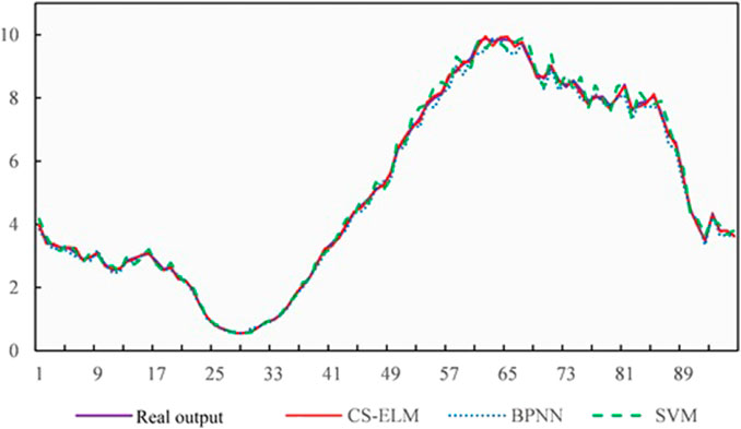
FIGURE 1. Calculation process of EEMD-CS-ELM.

(1) Set the CS algorithm parameters. Set the probability parameter $p_a$, which refers to the nest being discovered, generate N initial nest locations $nes{t}_0=\left[x_1^0,x_2^0,\dots ,x_N^0\right]$, which can be N different values of ELM hidden layer nodes after rounding up to an integer. Input the sample and calculate the root mean square error (RMSE) of the data as the most appropriate fitness value $F_0$, and the maximum number of iterations is $\max \_it$.

(2) Select the optimal nest location $x_i$ in the last time, search for nest location $j$ according to the mechanism of Lévy flight, and round up the number of nest locations as the number of ELM hidden layer nodes. Calculate the number of $F_j$ and compare with $F_i$, preserving the optimal fitness.

(3) Compare random number $p_r$ with $p_a$. If $p_r>p_a$, then choose the nest location randomly and replace the worst nest location; otherwise, make no change.

(4) Stop the search after the number of iterations is satisfied.

(5) Select the point with the least fitness as the number of hidden layer nodes $M$ for ELM, and output the corresponding W, b, and β

3.2 Optimization model of VPP in day-ahead trading considering CVaR

The CVaR value can be improved according to the deviation between the forecasted and actual output of wind and PV power. The deviation of output of wind power can be expressed as follows:

$g_{wpp}^{\prime }=g_{wpp}-g_{wpp}^f(27)$

If the forecasted deviation of output of wind power obeys the normal distribution, the probability density function will satisfy:

$f\left(g_{wpp}^{\prime }\right)=\frac{1}{\sqrt{2\pi }{\sigma }_{wpp}}{e}^{-\frac{g{\prime }_{wpp}^2}{2{\sigma }_{wpp}^2}}(28)$

The PV output is the same:

$f\left(g_{pv}^{\prime }\right)=\frac{1}{\sqrt{2\pi }{\sigma }_{pv}}{e}^{-\frac{g{\prime }_{pv}^2}{2{\sigma }_{pv}^2}}(29)$

Considering that both wind and PV units are necessary components for the VPP, the output curve can be regarded as the common output, and to simplify model calculation, the deviation of the common output can be expressed as follows:

${\phi }_{wpp,pv}=g_{wpp,pv}^{*}\left(t\right)-E\left[g_{wpp,pv}^{*}\left(t\right)\left|g_{wpp,pv}^{*}\left(t\right)\le Va{R}_{\alpha }\right.\left(g_{wpp,pv}^{*}\left(t\right)\right)\right](30)$

where ${\phi }_{wpp,pv}$ is the forecasted deviation of combined wind and PV output.

At this point, since there is no connection between the output characteristics of wind and PV, according to the convolution formula, the probability density distribution of $g_{wpp,pv}^{*}$ is shown as follows:

$f\left(z\right)=f\left(g_{wpp,pv}^{*}\right)=\frac{1}{\sqrt{2\pi }\left(\sqrt{{\sigma }_{wpp}^2+{\sigma }_{pv}^2}\right)}*e^{-\frac{{\left(g_{wpp}^{\prime }+g_{pv}^{\prime }\right)}^2}{2\left({\sigma }_{wpp}^2+{\sigma }_{pv}^2\right)}}(31)$

and,

$CVa{R}_{\alpha }=\frac{\sqrt{{\sigma }_{wpp}^2+{\sigma }_{pv}^2}}{\alpha }f\left(c\left(\alpha \right)\right)(32)$

where $c\left(\alpha \right)$ is the percentile of standard normal distribution α.

Considering that the main purpose of the VPP’s participation in the day-ahead market is to increase the proportion of distributed energy (such as wind power, PV) in power market, a demand response (DR) mechanism and a controllable burden, such as energy storage system (ESS), are introduced into the VPP to balance the generation fluctuation. In VPP, wind power plant (WPP) PV units and micro-turbine (MT) form a larger power resource, which reaches the power market access standard. When the generation side of the distributed renewable energy generating unit is connected to ESS, it will combine with the flexibility of the storage system, which charges when the load is low and discharges when the load reaches the peak, thus reducing the positive deviation power in the bid of the VPP. It will also reduce the penalty cost of electricity deviation in the settlement of the day-ahead market by using the energy storage units and interruptible load mechanism to sell power and transfer part of the load when there is minus deviation in the bidding (Figure 2).

FIGURE 2

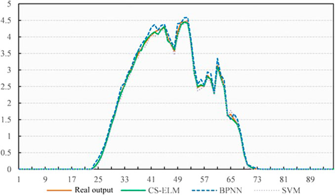
FIGURE 2. Structure of VPP.

Considering the trading rules of the day-ahead market, the VPP declares its generation plan the day before the operation day. The capacity of the VPP is small, and its market competitiveness is weak, which leads to a “price acceptor” in the market. Therefore, the market only needs to consider the declaration of the VPP when analyzing the day-ahead declaration behavior.

Based on the composition of the VPP in Figure 2 and the transaction flowchart of taking part in the day-ahead market in Figure 3, to realize the integration and scheduling of distributed energy, the absorption level of renewable energy in the VPP is considered, as well as the benefits. As the market price acceptor, the VPP can reduce operating costs to obtain more market benefits. After declaring a power generation plan, the ISO integrates and optimizes all quoted prices/numbers in the market to form a new power generation plan. Combined with the power generation plan given by the ISO, the VPP adjusts its power generation operation according to the target. The flow of VPP taking part in the day-ahead market is shown in Figure 3.

FIGURE 3

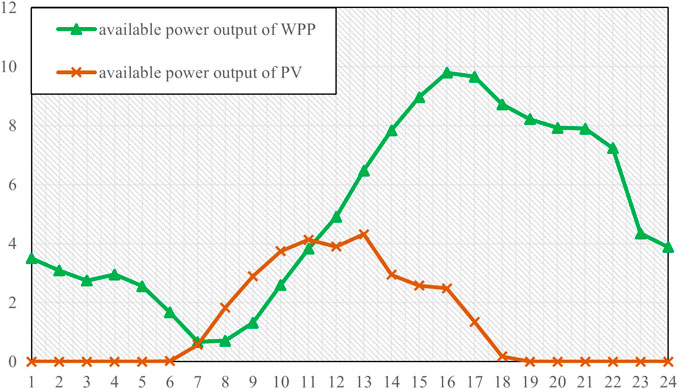
FIGURE 3. Trading process of VPP participating in day-ahead market.

Combined with the trading demand of VPP in the day-ahead market, the objective function can be expressed as:

$F_1^{DA}=\max \left(Q_{WPP}^{DA}+Q_{PV}^{DA}\right)(33)$

$F_2^{DA}=\min C_{VPP}^{DA}(34)$

$C_{VPP}=C_{ESS}+C_{WPP}+C_{PV}+C_{DR}+C_{MT}(35)$

$C_{WPP}={\displaystyle \sum _{t=1}^T}{C}_{t,o}^{WPP}+C_z^{WPP}+g_{WPP}^{\prime }·p_{WPP}(36)$

$C_{PV}={\displaystyle \sum _{t=1}^T}{C}_{t,o}^{PV}+C_z^{PV}+g_{PV}^{\prime }·p_{PV}(37)$

$C_{MT}={\displaystyle \sum _{t=1}^T}\left(a_{MT}{P}_{MT,t}^2+b_{MT}{P}_{MT,t}+c_{MT}\right)(38)$

$C_{ESS}={\displaystyle \sum _{t=1}^T}\left(p_t^{D,ESS}*Q_t^{char}+C_{t,o}^{ESS}\right.)(39)$

Here, $C_{t,o}^{WPP}$ and $C_{t,o}^{PV}$ refer to the operation cost of wind and PV units in period t, respectively; $C_z^{WPP}$ and $C_z^{PV}$ refer to the depreciation cost of wind and PV units, respectively; $g_{WPP}^{\prime }·p_{WPP}$ and $g_{PV}^{\prime }·p_{PV}$ refer to the deviation cost of wind and PV units, respectively; $a_{MT}$, $b_{MT}$, and $c_{MT}$ refer to the cost parameters of $M_t$ units; $p_t^{D,ESS}$ refers to the ESS power price at time t; $Q_t^{char}$ refers to the amount of ESS purchasing power at time $t$; and $C_{t,o}^{ESS}$ refers to the operating cost of energy storage at time $t$.

In the process of solving the model, constraints such as the balance of market supply and demand and unit operation are considered, as follows:

3.2.1 Constraints on power supply and demand balance in the day-ahead market

$D=Q_{WPP}^D+Q_{PV}^D+Q_{ESS}^D(40)$

Here, D is the load demand, $Q_{WPP}^D$ refers to the actual contribution of wind units, $Q_{PV}^D$ refers to the actual contribution of photovoltaic units, and $Q_{ESS}^D$ refers to the contribution of ESS in the day-ahead market. Because of the demand response, the power price will change and the capacity will shift, but the capacity will not actually change.

3.2.2 Unit operation constraint

Given that the energy supply cannot exceed the maximum allowable capacity of the generating units, the operating units of the power producers still need to meet the following constraints:

(1) Wind power generation constraints

$0\le P_{t,WPP}\le P_{t,WPP}^{\max }(41)$

Here, $P_{t,WPP}^{\max }$ is the maximum generation of WPP at time $t$.

(2) PV power generation constraint

$0\le P_{t,PV}\le P_{t,PV}^{\max }(42)$

Here, $P_{t,PV}^{\max }$ is the upper limit of PV units.

(3) MT unit constraint

For MT units, the main considerations are the output power and ramp constraints:

$P_{MT,t}^{\min }\le P_{MT,i}\le P_{MT,t}^{\max }(43)$

$P_{MT}^{down}\le P_{MT,t+1}-P_{MT,t}\le P_{MT}^{up}(44)$

where $P_{MT,t}^{\min }$ and $P_{MT,t}^{\max }$ are the lower and upper limit of MT at time $t$, respectively, and $P_{MT}^{down}$ and $P_{MT}^{up}$ are the uphill and downhill climbing power.

(4) ESS constraints

$0\le P_t^{ESS,char}\le {\delta }_s{P}_{\max }^{ESS,char}(45)$

$0\le P_t^{ESS,dis}\le \left(1-{\delta }_s\right)P_{\max }^{ESS,dis}(46)$

$E^{\min }\le E_t\le E^{\max }(47)$

Here, $P_{s\_char}^{\max }$ is the maximum charging efficiency and $P_{s\_dis}^{\max }$ is the maximum discharging efficiency of ESS; ${\delta }_s$ refers to the running status of ESS, and the charging and discharging situation cannot happen at the same time; $E^{\min }$ and $E^{\max }$ refer to the minimum and maximum of ESS, respectively; and $E_s^{t\_after}$ is the power storage after and $E_s^{t\_before}$ is the power storage before a dispatching cycle.

3.3 Solution of multi-objective optimization model based on ant colony optimization

The optimal transaction model of the VPP in the day-ahead market includes the goals of minimizing cost and maximizing renewable energy absorption. Given the constraints of unit technology, operation, and electric quantity, it is difficult to work out by a general calculation method. Ant colony optimization is a biomimetic algorithm based on the natural foraging behavior of ant colonies. In ant colony optimization, the path that an ant traverses represents a feasible solution to the problem, and all existing paths constitute the feasible solution space for the optimization problem. Ants with shorter paths can release more pheromones, and then more ants will choose those paths. After a few iterations, it will filter out a global optimal path. In the foraging behavior of an ant colony, the communication factor comprises only the pheromone concentration, which gives ant colony optimization strong global search ability, and it is a distributed parallel optimization. Consequently, the global search ability of ant colony optimization can be better used to solve the multi-objective trade optimization problem of a virtual power plant.

When ant colony optimization is used to solve the multi-objective optimal transaction model of a virtual power plant, the main parameters are the probability of individual state transition of ants and the updating rules of pheromones.

3.3.1 Probability of state transition

During the foraging process of an ant colony, the behavior of ants is influenced by the pheromone concentration, and their path choice will change accordingly. The probability of ant $a$ moving from node $i$ to node $j$ can be expressed as:

$P_{ij}^a\left(t\right)=\left\{\begin{array}{cc}\frac{{\tau }_{ij}^{\alpha }\left(t\right){\eta }_{ij}^{\beta }\left(t\right)}{{\displaystyle \sum }_{s\in S_a^c}{\tau }_{ij}^{\alpha }\left(t\right){\eta }_{ij}^{\beta }\left(t\right)},& j\in S_a^c\left(t\right)\\ 0& \mathrm{o}\mathrm{t}\mathrm{h}\mathrm{e}\mathrm{r}\mathrm{w}\mathrm{i}\mathrm{s}\mathrm{e}\end{array}\right.(48)$

where ${\tau }_{ij}\left(t\right)$ is the pheromones on the path on which ant $a$ is moving from node $i$ to node $j$ at time $t$; ${\eta }_{ij}\left(t\right)$ refers to the expectation that the ant will choose to move from node $i$ to node $j$, and the longer the path, the cheaper the optimal solution, which means the smaller the expectation; and $S_a^c\left(t\right)$ refers to the distances that ant $a$ can reach when moving from node $i$ to node $j$.

3.3.2 Pheromone update rules

When each ant reaches the food point, it will leave pheromones on the path it travels, that is, the pheromone concentration on this path increases; the change in pheromones on this path can be expressed as follows:

${\tau }^{\prime }\left(a\right)=\left\{\begin{array}{cc}{\alpha }_1\Delta {\tau }_j\left(a\right)+\left(1-{\alpha }_1\right)\tau \left(a\right),& {\tau }_j>{\tau }_i\\ \left(1-{\alpha }_1\right)\tau \left(a\right),& {\tau }_j\le {\tau }_i\end{array}\right.(49)$

where ${\tau }^{\prime }\left(a\right)$ is the pheromone concentration of ant $a$ at the latest position, ${\alpha }_1$ is the volatility coefficient of the original pheromones on the path, $\Delta {\tau }_j\left(a\right)$ is the pheromones left by the ant choosing the optimal path in the current iteration, and $\tau \left(a\right)$ is the pheromones left by the ant choosing the optimal path in the last iteration.

The process of solving the day-ahead market trade optimization model of a virtual power plant by ant colony optimization is shown in Figure 4.

FIGURE 4

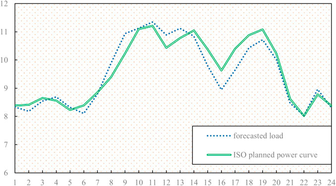
FIGURE 4. Process of solving ant colony optimization.

4 Study analysis

4.1 Forecast of wind and rain output based on EEMD-CS-ELM

For wind power sampling, the data of a 10 MW wind power station in northwest China from July 2019 was used as the training set, and the wind power output on 2 August 2019, was selected as the test set. The sampling of PV power units was based on data collected from June to July 2019 by the local PV power stations with a total capacity of 5 MW, and August 3 was chosen as the forecast date.

EEMD was used to decompose the power signal sequence of the selected wind power and PV output. Due to the poor stability of the photovoltaic power generation power sequence in rainy and snowy or cloudy weather, in order to fully reflect the objectivity of the scheduling characteristics of the virtual power plant in the day ahead market, take the wind power output in normal weather as an example, input the EEMD model, and a total of 12 components and a residual component are decomposed. After the PV sequence was decomposed, 10 IMF components and a residual component R were obtained. The decomposition results of wind power and photovoltaic output power series are shown in Figures 5, 6.

FIGURE 5

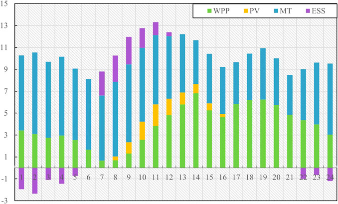
FIGURE 5. Decomposition sequence of wind power output.

FIGURE 6

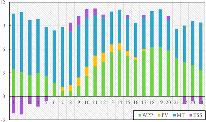
FIGURE 6. Decomposition sequence of PV output.

To verify the feasibility of the method proposed in this paper, BPNN, SVM, and CS-ELM forecasting models were selected for comparison, as shown in Figure 7. Among them, Back Propagation Neutral Network (BPNN) is a multilayer feed-forward network trained using an error back propagation algorithm, and is one of the most widely used networks at present. BPNN can learn and store a large amount of input-output mapping relationships without revealing mathematical equations in advance. The learning rule is to use the steepest descent method to continuously adjust the network weight and intrusion value through back propagation. The output value corresponding to the smallest mean square deviation of the network is the forecasted value. Support Vector Machine (SVM) uses correlation learning algorithm to transform them into high-dimensional feature space sample data when dealing with nonlinear problems. And then SVM carries out secondary classification to solve the segmentation hyperplane that maximizes the separation distance.

FIGURE 7

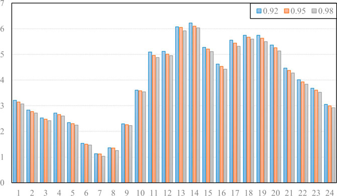
FIGURE 7. Forecasting results of wind power and PV output under different methods (MWh).

After the results were obtained, the mean average percentage error (MAPE), root mean square error (RMSE), and determination coefficient (R²) were used as indicators to evaluate the effect of the forecasting model, and the forecasting results were tested. MAPE can reflect the overall level of error and RMSE can reflect the dispersion of error. MAPE and RMSE are expressed as follows:

$RMSE=\sqrt{\frac{1}{n}{\displaystyle \sum _{i=1}^n}{\left(x_i-x_i^{\prime }\right)}^2}(50)$

$MAPE=\frac{1}{n}{\displaystyle \sum _{i=1}^N}\left|\frac{x_i^{\prime }-x_i}{x_i}\right|\times 100\%(51)$

$R^2=\frac{{{\displaystyle \sum _{i=1}^n}\left(p_i^{\prime }-\overline{p_i}\right)}^2}{{{\displaystyle \sum _{i=1}^n}\left(p_i-\overline{p_i}\right)}^2}(52)$

where $x_i$ is the actual power output, $x_i^{\prime }$ is the forecasted power output, and $n$ is the data volume. The RMSE, MAPE, and R2 values for each method are shown in Tables 1, 2.

TABLE 1

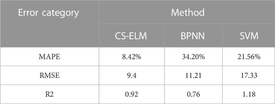
TABLE 1. Wind power forecast error test.

TABLE 2

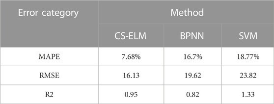
TABLE 2. PV forecast error test.

It can be seen from Tables 1, 2 that the proposed CS-ELM performs well in the three error test indicators. Its forecasting accuracy is higher than the other models, and its error indicators are smaller, further proving the effectiveness of the model.

4.2 Analysis of day-ahead transaction results of VPP

When the VPP participates in day-ahead market transactions, its internal wind and PV power output needs to meet the optimal overall economic benefits, effectively realizing the goal of maximizing the benefits. Therefore, combined with the CVaR risk value theory, considering the penalty factor brought by the risk in the objective function, objective function 2 of VPP can be written as follows:

$F_2^D=\max \left(C_{VPP}+{\phi }_{wpp,pv}·\lambda \right)(53)$

where $\lambda$ is the penalty factor in the risk penalty item when considering the risk of wind power output deviation.

Combined with the forecasting results, a 10 MW energy storage device and 10 WM micro gas turbine were connected to analyze the day-ahead trading behavior of the VPP considering the uncertainty risk, and the day-ahead trading results of the VPP were calculated with confidence levels of 0.92, 0.95, and 0.98. The energy consumption parameters of the MT unit are RMB 2.5/MW2, RMB 30/MW, and RMB 0, respectively, the climbing rate is 3 MW/h, and the failure rate is 0.5% (Gao, 2019). The price of wind power is about RMB 234/MWh, the price of photovoltaic is RMB 276/MWh, the initial capacity of the energy storage device is 1.5 MWh, and the charging and discharging efficiency is 0.95. The time scale of the wind forecast is 15 min in the day-ahead market transaction, and further analysis was carried out based on the average forecast output of wind point and PV within 1 h, as shown in Figure 8.

FIGURE 8

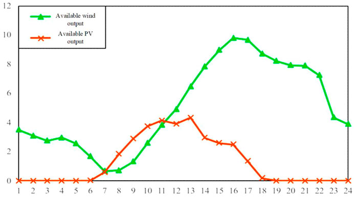
FIGURE 8. WPP and PV output forecast (MWh).

Due to the small capacity of distributed generation, the VPP has a small volume in the power market transaction, which has little impact on the market clearing. It is often used as a “price receiver” in the market. Therefore, the bidding behavior of the VPP in the day-ahead market is only considered through the reported volume.

The clearing price of the day-ahead market is based on the market operation results of the Nordic market on a certain day in April 2020. The load forecast of the VPP for the next day’s market and the power generation plan after ISO adjustment are shown in Figure 9.

FIGURE 9

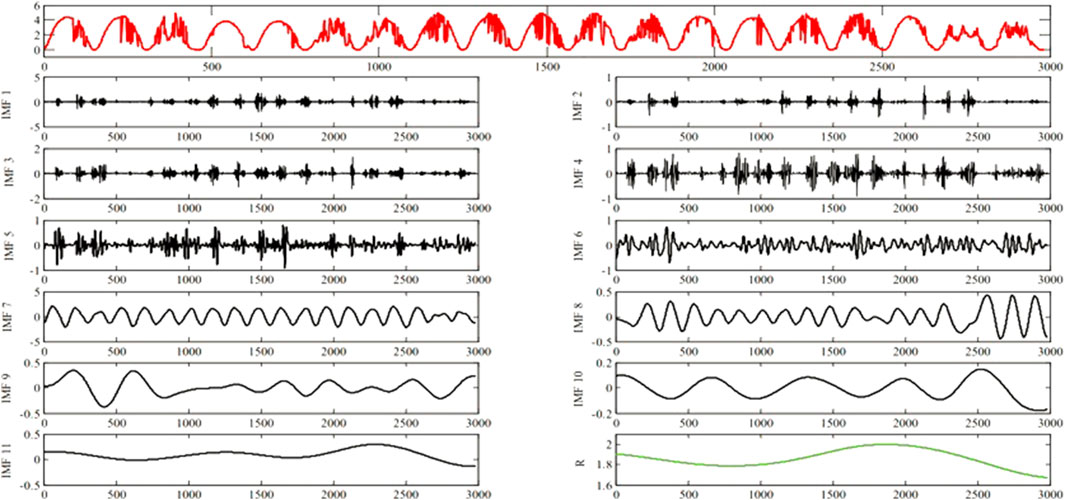
FIGURE 9. Load forecast of day-ahead market (MWh).

The VPP declares its output according to the load forecasting results of the day-ahead market. Its internal operation is scheduled according to the double objective function of minimizing cost and maximizing renewable energy consumption. The declaration of various units is shown in Figure 10.

FIGURE 10

FIGURE 10. Output arrangement of VPP in day-ahead market (MWh).

After the declaration, the market ISO makes a collective adjustment in combination with the declared output and power plan of each power producer and releases the updated output plan. The virtual power plant adjusts the output arrangement of each unit in combination with the updated output plan and objective function. At this time, the overall declaration curve tends to be smoother. The final output arrangement is shown in Figure 11.

FIGURE 11

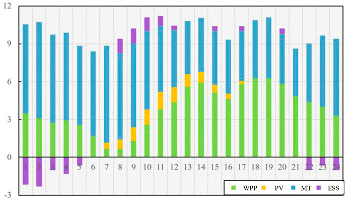
FIGURE 11. Final output arrangement of VPP in day-ahead market (MWh).

According to Figures 9–11, when the virtual power plant adjusts the generation plan, the curves of MT units and ESS changes the most, which is also due to the uncertainty related to wind and solar output and the characteristics of rapid adjustment of the MT units and energy storage devices. In addition, in combination with Figures 8, 9, it can be seen that the declared output of WPP is somewhat different from the available output when VPP is declaring the power generation plan. And the PV generation curve changes the least. This is because the cost of wind turbine units is higher than that of MT units, and the related standby cost to overcome the uncertainty of wind turbine units is also considered. At this time, the total operating cost of the reported generation plan of the virtual power plant is RMB 50,846.65.

4.3 Influence of confidence levels on optimization results of day-ahead VPP transactions

In addition, considering the risk preference of the VPP, scenarios were set at different confidence levels to analyze the operating costs of the VPP. Based on the risk analysis of the VPP’s participation in the day-ahead market, the generation deviation of WPP and PV has a certain impact on the VPP’s day-ahead transactions. In order to deal with the uncertainty of wind power generation, the VPP will increase the corresponding reserve capacity to reduce market risk. Therefore, the day-ahead trading results of a virtual power plant with confidence levels of 0.92, 0.95, and 0.98 were selected for further analysis from Table 3.

TABLE 3

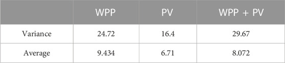
TABLE 3. Wind power and PV output distribution.

It can be seen from Table 4 that as the confidence level increases, the VPP provides backup services for distributed wind power and PV output by using ESS and MT units to deal with the uncertainty of renewable energy output, resulting in rising costs. It can be seen from Figure 12 that as the confidence level improves, the trading volume of distributed renewable power in the day-ahead market decreases to a certain extent; that is, to reduce the uncertainty and scale of wind power, the penalty cost is further reduced by reducing the deviation between planned and actual output. Therefore, when participating in the day-ahead market, the VPP needs to comprehensively consider the output and confidence level of distributed wind and power so as to further realize coordination and balance between economic concerns and risk avoidance.

TABLE 4

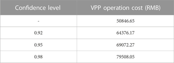
TABLE 4. Operation cost analysis of VPP with different confidence levels.

FIGURE 12

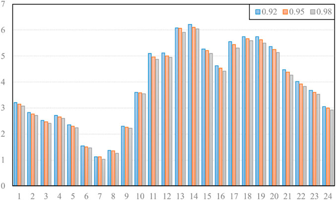
FIGURE 12. Comparison of distributed renewable energy output with different confidence levels (MWh).

5 Conclusion

This paper focuses on uncertainty analysis of a VPP in the day-ahead power market. First, the sources of uncertainty were divided into two types, and a way to reduce uncertainty was designed for each one. Then, the inner uncertainty of the VPP was solved though the EEMD-CS-ELM forecasting model of new energy (wind and PV). At the same time, CVaR theory was introduced to measure the risk of deviation between the planned power generation and the actual load demand of the market, and a day-ahead trading optimization model considering CVaR method was built. The ant colony algorithm for multi-objective optimization was introduced to solve the two-sided optimal uncertainty question. To verify the proposed model, a case study was designed, and the results show the following: 1) the forecasting model is more efficient than the traditional algorithm in terms of accuracy, and 2) the confidence levels are not fully positive with the benefit of VPPs. Improving the confidence level could reduce the uncertainty brought by renewable energy, but could also cause conservative trading behavior and affect the consumption of renewable energy. Therefore, to perform better in the day-ahead power market, VPPs should improve the forecasting accuracy at the outset and determine the appropriate risk preference to design a diversified quotation strategy with full consideration of regulatory resources such as energy storage and demand response. Based on the research results of this paper, further research will focus on market transactions with shorter time scales, combined with VPP’s flexible regulatory ability, to explore more suitable spot market quotation methods and transaction categories for VPP’s flexible power supply.

Data availability statement

The original contributions presented in the study are included in the article/Supplementary Material, further inquiries can be directed to the corresponding authors.

Author contributions

Conceptualization, WJ and WQ; methodology, GW; software, WQ; validation, LH, GW, and WQ; formal analysis, WJ; investigation, GW; resources, GW; data curation, WQ; writing—original draft preparation, WQ; writing—review and editing, LH; visualization, GW; supervision, WQ; project administration, WJ. All authors contributed to the article and approved the submitted version.

Funding

Project Supported by Science and Technology Project of Taizhou Science and Technology Bureau (21gya31), Science and Technology Project of Zhejiang Provincial Department of Housing and Urban-Rural Development (2020K165), Special project for basic scientific research business funds of central public welfare scientific research institutes (1610332022009); 2021 Inner Mongolia Autonomous Region Talent Introduction Research Support Project, Inner Mongolia Autonomous Region Higher Education Institutions “Young Science and Technology Talents” Project (NJYT-20-A19); Ordos Industrial Innovation and Entrepreneurship Talent Team Project: Ordos City Ecological Restoration and High-quality Development of Cultural Tourism Industry.

Acknowledgments

The completion of this paper has been helped by all authors. We would like to express our gratitude to them for their help and guidance.

Conflict of interest

Author GW was employed by Era Co.,Ltd. WJ was employed by Electric Power Planning and Design Institute Co., Ltd.

The remaining authors declare that the research was conducted in the absence of any commercial or financial relationships that could be construed as a potential conflict of interest.

Publisher’s note

All claims expressed in this article are solely those of the authors and do not necessarily represent those of their affiliated organizations, or those of the publisher, the editors and the reviewers. Any product that may be evaluated in this article, or claim that may be made by its manufacturer, is not guaranteed or endorsed by the publisher.

References

Bai, K., Gu, J., Peng, H., and Zhu, R. (2018). Optimal allocation for multi-energy complementary microgrid based on scenario generation of wind power and photovoltaic output. Automation Electr. Power Syst. 42 (15), 133–141.

Google Scholar

Dong, G., Zhang, H., Wang, Z., and Xiong, Y. (2018). Research on the electric vehicle charging load forecasting based on the uncertainty of response behavior. Electr. Meas. Instrum. 55 (20), 60–65.

Google Scholar

Duan, P., Zhu, J., and Liu, M. (2016). Optimal dispatch of virtual power plant based on Bi-level fuzzy chance constrained programming. Trans. China Electrotech. Soc. 31 (9), 58–67.

Google Scholar

Fan, S., Qian, A., and He, X. (2015). Risk analysis on dispatch of virtual power plant based on chance constrained programming. Proc. CSEE 35 (16), 4025–4034.

Google Scholar

Gao, Z. (2019). Study on bidding strategy and coordinated dispatching of virtual power plants with multiple distributed energy sources. Shanghai, China: Shanghai Jiao Tong University.

Google Scholar

Heydarian Forushani, E., Moghaddam, M. P., Sheikh-El-Esalmmk, M. K., Shafie-khah, M., and Catalao, J. P. S. (2014). Risk-constrained offering strategy of wind power producers considering intraday demand response exchange. IEEE Trans. Sustain. Energy 5 (4), 1036–1047. doi:10.1109/tste.2014.2324035

CrossRef Full Text | Google Scholar

Jadfari, A. M., Zareipour, H., Achellengberg, A., and Amjady, N., (2014). The value of inrea-day markets in power systems with high wind power penetrations. IEEE Transaction Power Syst. 29 (3), 1121–1132.

Google Scholar

JafariZareipourSchellenberg, A. M. H. A., and Amjady, N. (2014). The value of intra-day markets in power systems with high wind power penetration. IEEE Trans. Power Syst. 29 (3), 1121–1132. doi:10.1109/tpwrs.2013.2288308

CrossRef Full Text | Google Scholar

JuTanYuan, L. Z. J., Tan, Q., Li, H., and Dong, F. (2016). A bi-level stochastic scheduling optimization model for a virtual power plant connected to a wind–photovoltaic–energy storage system considering the uncertainty and demand response. Appl. Energy 1717, 184–199. doi:10.1016/j.apenergy.2016.03.020

CrossRef Full Text | Google Scholar

Kong, B., Cui, L., Ding, Z., and Li, X. (2015). Short term power prediction based on hybrid wind-PV forecasting model. Power Syst. Prot. Control 43 (18), 62–66.

Google Scholar

Li, L., Qiu, X., Zhang, H., Zhao, Y., and Zhang, K. (2021). Risk aversion model and profit distribution method of virtual power plant in power market. Electr. Power Constr. 42 (1), 67–75.

Google Scholar

Liu, D., Ma, G., Tao, C., and Wang, J., (2020). Electricity prices distribution characteristics and volatility risk measurement in the PJM power market. Power Syst. Clean Energy 36 (9), 15–21.

Google Scholar

Meibom, P., Barth, R., Hasche, B., Brand, H., Weber, C., and O'Malley, M. (2011). Stochastic optimization model to study the operational impacts of high wind penetrations in Ireland. IEEE Transaction Power Syst. 26 (3), 1367–1379. doi:10.1109/tpwrs.2010.2070848

CrossRef Full Text | Google Scholar

Niu, D., Wang, K., and Wu, J. (2020). Can China achieveits 2030 carbon emissions commitment? Scenario analysis based on an improved general regression neural network. J. Clean. Prod. 243 (10), 118558–118558.

CrossRef Full Text | Google Scholar

Pinson, P., Chenallier, C., and Kariniotakis, G. N. (2007). Trading wind generation from short-term probabilistic forecasts of wind power. IEEE Transaction Power Syst. 22, 1148–1156. doi:10.1109/tpwrs.2007.901117

CrossRef Full Text | Google Scholar

Riveraion, J. Z., Bruninx, K., Poncelet, K., and D’haeseleer, W. (2015). Bidding strategies for virtual power plants considering CHPs and intermittent renewables. Energy Convers. Manag. 103, 408–418. doi:10.1016/j.enconman.2015.06.075

CrossRef Full Text | Google Scholar

Shayegan-Rad, A., Badri, A., and Zanganeh, A. (2017). Day-ahead scheduling of virtual power plant in joint energy and regulation reserve markets under uncertainties. Energy 121, 114–125. doi:10.1016/j.energy.2017.01.006

CrossRef Full Text | Google Scholar

Shu, G., He, P., and Ma, R. (2020). Multi-time scale unit combination method considering precision characteristics of wind power and solar power forecasting. Electr. Power Eng. Technol. 39 (3), 78–83.

Google Scholar

Sun, J., Hu, J., and Fang, W. (2021). Active distribution network power admission capacity planning based on improved scene clustering method. Sci. Technol. Eng. 21 (1), 194–200.

Google Scholar

Tan, J., and Yang, L. (2019). Review on transaction mode in multi-energy collaborative market. Proc. CSEE 39 (22), 6483–6497.

Google Scholar

Wu, J., Xue, Y., Shu, Y., and Xie, D. (2019). Adequacy optimization for a large-scale renewable energy integrated power system Part Three: Reserve optimization in multiple scenarios. Automation Electr. Power Syst. 43 (11), 1–7+76.

Google Scholar

Zamani, A. G., Zakariazadeh, A., and Jadid, S. (2016). Day-ahead resource scheduling of a renewable energy based virtual power plant. Appl. Energy 169, 324–340. doi:10.1016/j.apenergy.2016.02.011

CrossRef Full Text | Google Scholar

Zhang, J., Jiang, F., Wu, H., and Qi, X. (2020). Dual market bidding strategy of load aggregator based on CVaR. Electr. Power Autom. Equip. 40 (12), 153–158.

Google Scholar

Zhang, Y., Lu, H. H., Fernando, T., Yao, F., and Emami, K. (2015). Cooperative dispatch of BESS and wind power generation considering carbon emission limitation in Australia. IEEE Transations Industrial Inf. 11 (6), 1313–1323. doi:10.1109/tii.2015.2479577

CrossRef Full Text | Google Scholar

Zhou, X., Zeng, R., Gao, F., and Lu, Q. (2017). Development status and prospects of the energy internet. Sci. China Inf. Sci. 47 (2), 149–170.

CrossRef Full Text | Google Scholar

Zhu, W., and Xie, P. (2015). Influence analysis of CVaR model based TOU electricity price on portfolio strategy. Power Syst. Prot. Control 43 (14), 16–21.

Google Scholar